Abstract
With the rapid development of meteorological models, numerical weather prediction is increasingly used in flood forecasting and reservoir regulation, but its forecasting ability is limited by the large amount of uncertainty from meteorological systems. In this paper, a new, hybrid framework is developed to improve numerical precipitation forecasting by combining the multimodel ensemble and probabilistic postprocessing methods. The results show that the multimodel ensemble method used in this paper is an efficient way to reduce prediction errors, especially missing alarm errors. In a comparison of the probabilistic postprocessors based the generalized Bayesian model (GBM) and bivariate probabilistic model (BPM), the GBM shows better performance from the aspects of indicators and is more suitable for real-time applications. Meanwhile, the assessment of probabilistic results shows that the skill of probabilistic precipitation forecasts is related to the quality of their inputs. According to these results, a new hybrid framework is proposed by taking the results from multimodel ensemble as the input of probabilistic postprocessor. Compared to using the raw numerical in GBM, the hybrid framework improves the accuracy, sharpness, reliability, and resolution ability from different lead times by 2–13%, 1–22%, and 0–12% respectively, especially when the lead time is less than 4 d, the improvement can reach 9–13%, 10–22%, and 5–12% respectively. In conclusion, the hybrid two-step framework can provide a more skillful precipitation forecast, which can be useful for flood forecasting and reservoir regulation.
1. Introduction
Due to the influence of the monsoon climate, many areas in China face a shortage of freshwater during the dry season, and a threat of flood disasters in the wet season [1,2,3]. Many previous studies have pointed out that flood forecasting is one of the key techniques for reducing flood damage. However, flood forecasts based on hydrological models forcing by ground stations or remote sensing have very limited lead times, i.e., the time from the first observation of rain to the occurrence of a flood peak can only provide a small amount of future information and makes it difficult to support reservoir regulation decisions [4,5]. It still remains a challenging task for providing reliable flood forecasts with long lead times. As mentioned in many previous studies, numeric precipitation forecast (NPF) is an effective way to extend the lead time for flood forecasting [6,7].
Flood forecasting based on hydrological models forcing by observed precipitation and NPF has a longer lead time and enables the development of reservoir regulation strategies in advance [8,9]. However, due to the uncertainty of meteorology systems, rainfall forecasting generally exhibits errors that affect the accuracy of flood forecasting from hydrological models and subsequently may be detrimental to flood control safety [10,11,12]. Therefore, rainfall information from NPF has still not been fully utilized in hydrological forecasting. In recent years, a number of researchers have employed different postprocessing methods to reduce the prediction errors of raw NPFs [13,14]. Multimodel ensembles are commonly used methods that build a relationship between independent predictions from different data sources/models and observations [15]. Both linear and nonlinear regression methods have been applied to numerical weather forecasting. Linear models, such as the linear regression, bias-removed ensemble mean (BREM), have been suggested to improve the skill of raw weather forecasts [16,17]. Artificial neural networks (ANNs) and support vector machines (SVMs) are the two most popular nonlinear methods for multimodel ensemble forecasting [18]. However, most of these models only focus on the difference between the true value and forecast value, such as the mean absolute error (MAE) or root mean square error (RMSE), but neglect the different impacts of false alarm (FA, events that were forecasted but did not occur) and missing alarm (MA, events that were not forecasted but did occur) on flood control safety [19]. An FA only reduces the potential benefits of reservoir operation, while an MA may be detrimental to flood control safety. Therefore, it is necessary to pay more attention to MA errors rather than overall errors or FA errors.
The uncertainty of precipitation forecast is commonly evaluated by the conditional distribution obtained from probabilistic forecast models [20,21]. Most of these probabilistic models are based on a bivariate meta-Gaussian distribution developed by Krzysztofowicz and Kelly [22]. Herr and Krzysztofowicz first used this method to assess the uncertainty in precipitation data through a normal quantile transformation (NQT) [23]. Robertson et al. [24] proposed a rainfall postprocessing (RPP) method on the basis of the Bayesian joint probability approach by Wang and Robertson [25]. Tao et al. evaluated the performance of probabilistic forecasts from single-value precipitation forecasts by ensemble pre-processing (EPP) [26].
As shown in many former studies, the multimodel ensemble method based on machine learning models is an effective way to reduce the error of precipitation forecasts through a regression of independent predictions from different data sources, but most of these methods are deterministic and cannot describe the uncertainty in precipitation forecasts [27,28]. In contrast, probabilistic precipitation models can evaluate the uncertainty of single-value forecast results via a distribution analysis, and the forecast skill of the probabilistic results is related to the skill of the inputs. From the characteristics of these two methods, it is possible to obtain a better precipitation forecast by combining multimodel ensemble methods and probabilistic models. To be more specific, it may be feasible to employ the outputs from multimodel ensemble method, which has higher accuracy than the raw NPF, as the input of probabilistic precipitation models to generate more skillful probabilistic precipitation forecasts. However, most current studies only evaluated the improvement of precipitation forecasts by a single method, using multimodel ensemble method or probabilistic precipitation model, it is still unknown whether we can obtain a better probabilistic precipitation forecast by combining the two methods in a hybrid two-step framework.
The aim of this study is to establish a hybrid two-step framework to improve the performance of precipitation forecasting through a combined multimodel ensemble and probabilistic forecast, from the aspect of actual needs of flood forecast and reservoir regulation. We evaluate the daily control forecast of four forecasting centers from the TIGGE (THORPEX Interactive Grand Global Ensemble) over the Meishan Catchment in Huaihe Basin of China during the wet season (May to September). As a first step, a nonlinear multimodel ensemble method with special consideration for MA errors is adopted to reduce the prediction errors of raw NPFs. Then, two different probabilistic models, a bivariate probability model (BPM), and the generalized Bayesian model (GBM), are used for both the original and corrected results. Furthermore, we evaluate all the correction and probabilistic results to obtain a reliable hybrid two-step framework to improve the skill of the raw NPF in relation to flood forecast and reservoir regulation. Note that the focus of this study is not the comparison of single multimodel ensemble methods or probabilistic postprocessing methods, but the combination of the two. Therefore, only very limited methods are used in this study, but all these methods have been reported as effective methods to improve the performance of NPF in the previous studies [29,30].
2. Methods and Materials
2.1. Methodology
The main aim of postprocessing is to reduce the error of NPFs with different lead times. In this study, a nonlinear multimodel ensemble method and two probabilistic postprocessors are employed, and a combined framework is built to generate probabilistic precipitation forecasts with better performance. First, the control forecast from four different centers are used as the input of an SVR-based multimodel ensemble forecast model to improve the accuracy of raw NPF. Then the results of the ensemble forecast are input into a probabilistic post-processor to obtain the final probabilistic forecast results. The flow chart of the hybrid framework is shown in Figure 1. To evaluate the results of the postprocessors, several statistical metrics are employed, including the RMSE, average width of prediction intervals (WPI), and Brier score.
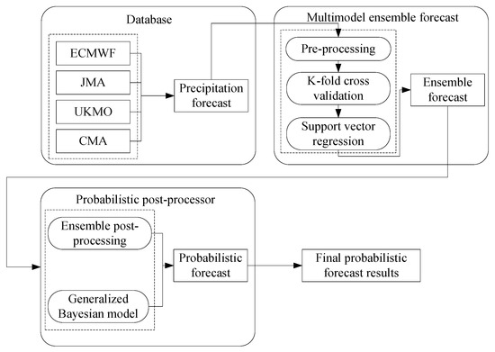
Figure 1.
Flow chart of the hybrid two-step framework for combining precipitation forecast postprocessors.
2.1.1. Verification Methods
The RMSE is employed to examine the performance of precipitation forecasting. The RMSE is one of the most popular indicators to quantify the extent to which a predicted response value is close to the true response value (Equation (1)). For probabilistic case, RMSEP is also employed to examine the accuracy of probabilistic postprocessing methods (Equation (2)).
where denotes the total number of forecasts and observations. and denote the th prediction and observation (true value) respectively, and is the conditional distribution of true value when the th prediction is available.
The WPI is a simple but effective measure of sharpness in probabilistic forecasting. Generally, it refers to the average width of a 90% prediction interval [31].
where represents the total number of forecasts and and represent the ith upper and lower bounds of the probability 0.90 prediction interval, respectively (Equation (4)).
The multicategory Brier score is often used as a measure of probabilistic forecast reliability and resolution ability, and can be calculated with the following equation [32,33]:
where represents the total number of samples, is the total number of classifications, denotes the forecasted probability of sample under the condition that th magnitude class occurs, and is equal to 1 if the true value of sample is th magnitude class, otherwise is equal to 0. The Brier score is negatively oriented with a range of 0 to 1, and the Brier score is equal to 0 when the forecast is perfect.
The magnitude classification of daily precipitation for multicategory Brier score is based on the classification standard of the meteorological department of China. Generally, no rain means that the daily precipitation is 0. However due to their limited influence on the formation of floods, precipitation levels under 1 mm are also considered to have a precipitation score of 0 in this study. The classification standard is detailed in Table 1.

Table 1.
Classification standard of daily precipitation from the meteorological department of China.
2.1.2. Multimodel Ensemble Method
Due to the spatial and temporal complexity of precipitation forecasting, it is almost impossible to develop a model that surpasses other models in all forecasting situations. An alternative way is to use multimodel ensemble forecasting, which can improve the forecast skill of NPF, prevent overconfidence of a single model, and reduce the errors by combining the strengths of the different models [34,35]. For a certain time , the results from an model are , and the corresponding observation is . The main purpose of the multimodel ensemble method is to find a function , that minimizes the loss function between and . The function in the multimodel ensemble method can be in any form, which may be linear or nonlinear and the loss function can be any indicator for performance evaluation, such as the RMSE or hit rate. A nonlinear multimodel ensemble method based on support vector regression (SVR) is used in this study, which proves that it can effectively reduce the error of MA events [29]. The SVM is a statistical learning method for classification and regression proposed by Vanpik et al. in 1995 based on the structural risk minimization principle [36]. Currently, SVR has been widely employed in hydrology and meteorology [37,38].
We use the ν-SVR method originally developed by Schölkopf et al. [39]; details of this method are provided in Appendix A. There are three parameters in ν-SVR that need to be optimized to determine: C, ν, and σ. C represents the cost constant, which is a compromise between the complexity and generalization of the model. By changing the value of C, we can adjust the ratio of the confidence range and empirical risk in the sample space and determine the penalty degree for the sample whose loss exceeds a threshold. The ν is the lower bound of the support vector and the upper bound of the gap error. The σ is a parameter of the radial basis function kernel, which is used to map the dataset from the original sample space to a higher dimensional space.
The three parameters can be determined based on an optimization algorithm, for example, the genetic algorithm (GA) or the particle swarm optimization algorithm (PSO), with a cost function that minimizes the overall error. However, an objective function aiming to minimize the overall error is not the preferred goal for flood control, where safety is more important. Therefore, in this paper, a special objective function (Equation (6)) is adopted for the ν-SVR model by minimizing the RMSE of MA events (SVR-MA).
where
In Equation (6) to Equation (9), is the th vector of precipitation forecasts from different centers, i.e., the input of multimodel ensemble method, is the corresponding observation, represents the output of multimodel ensemble method, and the is the sample size.
All the SVR models used in this paper are based on the open-source software, LIBSVM, developed by Chang and Lin [40]. More information about the SVR models is available at https://www.csie.ntu.edu.tw/~cjlin/libsvm/ (accessed on 14 April 2021).
2.1.3. Probabilistic Postprocessing Method
(1) Bivariate probability model
The bivariate probability model is used to generate probabilistic precipitation forecasts from a single-value raw NPF through a bivariate joint distribution. Currently, most probabilistic postprocessing models are based on a bivariate probability model by Herr and Krzysztofowicz, including the EPP by the U.S. National Weather Service [26] and the RPP by Robertson et al. [24]. The model contains two main steps: (1) deriving the joint distributions of raw forecasts and observations and (2) obtaining the conditional distributions of observations given the raw forecasts. Here, the statistical procedure developed by Wu et al. [41] is adopted.
Let denote the daily raw single-value precipitation forecast and be the corresponding observation (i.e., true value). The cumulative distribution function (CDF) of the conditional distribution can be written as:
Deriving the joint distribution of raw forecasts and observations requires the marginal distributions. However, unlike other meteorological variables, natural rainfall is generally characterized as an intermittent stochastic process with a mixed marginal distribution, including both discrete and continuous parts [42,43]. The discrete part is concentrated at zero representing the probability of no rain, while the continuous part might be described by a known continuous distribution, such as the gamma distribution and Weibull distribution, or derived from a nonparametric statistic. Finally, the marginal distribution of can be expressed as:
where .
Therefore, the joint distribution consists of four parts:
where
Since the conditional marginal CDFs of and are both continuous, their joint CDF, is also continuous. As introduced in Wu et al., the bivariate meta-Gaussian model is used to estimate . More detailed information about the bivariate meta-Gaussian mode can be obtained in [44,45,46,47,48].
With the joint distribution, the conditional CDF of can be expressed as Equations (13) and (14) for and respectively:
where and ; is the probability density function (PDF) of ; is the marginal PDF of when ; and .
(2) Generalized Bayesian model
The generalized Bayesian model was developed by Cai et al. for uncertainty analysis of single-value NPFs based on a Bayesian formula and generalized probability density function (GPDF) [30]. The Bayesian formula is an effective method for uncertainty analysis and is commonly used in probabilistic forecasting [49,50]. However, the traditional Bayesian formula is limited to characterizing the conditional distribution for either discrete or continuous random variables and is not suitable for mixed random variables such as precipitation. To solve this problem, the Dirac delta function (Equation (15)) is employed to transform the distribution laws of discrete random variables into a probability density function (PDF) form called a generalized PDF (GPDF).
Let represent a discrete random variable. All the possible values of are with corresponding probabilities , and . The CDF of can be expressed as:
where .
The GPDF of the discrete random variable X is defined as:
and:
Equations (17) and (18) show that the GPDF satisfies all the characteristics of the PDF, and discrete, continuous, and mixed distributions can be expressed in the form of the GPDF. Therefore, through the GPDF, the GBM can be used for mixed distributions. The first part of the GBM for precipitation forecasting is the prior distribution. Here, we use to represent the raw single-value precipitation forecast, and is the corresponding observation. In this study, the prior distribution is the marginal distribution of which is a mixed distribution and can be written as Equation (19):
The second part of the Bayesian formula is the likelihood function . For this case, the GPDF of the likelihood function should be divided into two parts because of the sample space of ; for and , the likelihood functions can be drawn as follows:
where and .
To estimate the distribution of the likelihood function (Equation (20)), the prediction error is introduced in this study:
Note that is nonnegative when due to the sample space of . Therefore, the continuous part for in Equation (20) is a nonnegative distribution. If , the errors between the forecasted value and unknown true value can generally be assumed to obey a censored normal distribution (Equation (22)):
where is a parameter guaranteeing a total probability of 1.
Since both the prior distribution and likelihood function can be expressed by the GPDF, it is easy to obtain a posterior distribution through the Bayesian formula:
2.2. Study Area
The Meishan Catchment is a subcatchment of the Huaihe River Basin in southeastern China, with a drainage area of 1970 km2. A large reservoir, the Meishan Reservoir, is located at the outlet of the basin, and is used for flood control, water supply, and hydropower generation (Figure 2). This catchment is in a typical monsoon-affected climatic zone, with precipitation concentrated from May to September (wet season). Meanwhile, as part of the Dabie Mountains, the elevation in this area varies greatly, which makes the area prone to flash floods. The basin experienced many major flood events in the past, which severely threatened the safety of the reservoir and downstream cities. In contrast, due to the economic and population growth in the area, the demand for water supply from the reservoirs has increased each year, especially during the dry season. Therefore, it is urgent to utilize more water resources without compromising flood control safety.
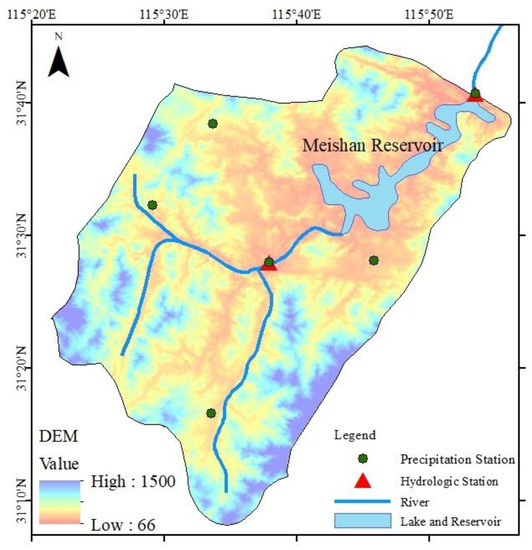
Figure 2.
The Meishan Catchment in the upper Huaihe River Basin and the location of the reservoir, hydrological station, and precipitation stations. From the digital elevation model (DEM) data, the elevation of the basin is shown to gradually decrease from south to north.
2.3. Data Sources
As a major component of The Observing System Research and Predictability Experiment (THORPEX), the TIGGE is a numeric weather forecasting dataset consisting of eleven main forecasting centers around the world since 2006. The main purpose of the TIGGE is to improve high-impact weather forecasting ability with a two-week lead time [51]. In this study, we select the control forecasts from four different centers, the European Center for Medium-Range Weather Forecast (ECMWF), Japan Meteorological Agency (JMA), United Kingdom Meteorological Office (UKMO), and China Meteorological Center (CMA). More details of these datasets are given in Table 2.

Table 2.
Configurations of the four TIGGE precipitation forecasts used in this study.
2.4. Experimental Design
The daily control forecasts of the four centers are used as raw NPFs. Since the horizontal resolutions and forecast lengths of the forecasts are different, a series of methods are needed to make the datasets consistent. In this case, only the forecasts with a base time of 00:00 UTC are selected, and the forecast lead is 7 d (168 h). The spatial resolution of all products is converted to 0.50° × 0.50°. For comparison with observed data from the ground sites, the precipitation forecast is averaged spatially with the gridded area as the weight. The areal average observations are measured from the precipitation stations in Figure 2 by using the Thiessen polygon method.
To build three models (i.e., SVR-MA, BPM, and GBM) used in this study, the parameters and distribution in the models should be determined. In this study, we adopted the data in the flood season during 2015–2017 as the training set, which determines all the parameters and distributions, while the data in 2018–2019 are used for testing.
The three parameters of SVR-MA are estimated by the PSO with five-fold cross validation. We first randomly divide the training samples into five categories. Then we use one of the categories as the validation set in order, and the rest as a training set and determine the best parameter settings through the PSO algorithm and Equations (6)–(9).
For the distributions of the continuous part in the probabilistic models, four nonnegative distributions, including gamma, lognormal, Weibull, and exponential distributions, are employed to fit the distribution for the precipitation forecasts and observation. The Kolmogorov–Smirnov test (K–S test) is adopted to test whether the distribution can be accepted and find the most suitable distribution, and maximum likelihood estimation (MLE) is used to determine the parameters of the distributions.
3. Results and Discussion
In this section, we assess the performance of three different postprocessing models and employ a new framework by combining a multimodel ensemble and probabilistic forecasting. The precipitation forecast data from May to September of 2015–2019 are used for training and verification. All results are compared to the raw forecasts from the TIGGE and/or the observations.
3.1. Verification of Multimodel Ensemble Forecasts
As a first step of this study, the performances of daily control forecast from the four centers and their ensemble results by the SVR-MA method are evaluated against area-weighted observations based on several statistical metrics. The SVR model with the target of minimizing MA error is used as the multimodel ensemble method. Figure 3 shows that, as measured by the RMSE, the JMA presents the best results for both the training and verification periods among the four raw NPFs, while the forecasts from the CMA have the lowest skill at most lead times. In general, the performance of all raw NPFs deteriorates with increasing lead time. The multimodel ensemble method shows a great improvement in accuracy during the training period, especially when the lead time is over 4 days. In the verification period, the performance of the SVR-MA model shows a decline, but it is still better than the original forecast results.
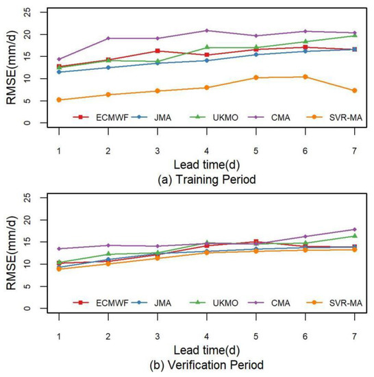
Figure 3.
The RMSE of the raw NPF and the SVR-MA model in the Meishan Catchment from May to September 2015–2019, where (a) represents the training period (2015–2017) and (b) represents the verification period (2018–2019).
Figure 3 indicates that the SVR-MA model can reduce the overall error, but its effect is limited in the verification period. As mentioned above, MA errors play a more important role in flood control systems, so it is necessary to examine the MA error of the forecasts. Figure 4, which shows the RMSE-MA values calculated from Equation (6) to Equation (9), shows that the multimodel method has a better performance in the training period and the SVR-MA model has the best forecast skill in the verification period. Meanwhile, the gap between the four raw NPFs becomes negligible, with the JMA forecasts showing no obvious advantage. Additionally, as shown in Figure 5, the number of MAs greatly decreases during the training and verification periods in the SVR-MA model. With the smallest MA error and the fewest MAs, the SVR-MA model demonstrates its ability to reduce underestimation from the NPF, which is more in line with the needs of flood forecast and reservoir regulation.
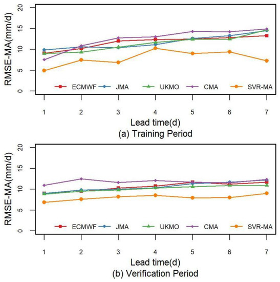
Figure 4.
The RMSE-MA of the raw NPF and the SVR-MA model in the Meishan Catchment from May to September 2015–2019, where (a) represents the training period (2015–2017) and (b) represents the verification period (2018–2019).
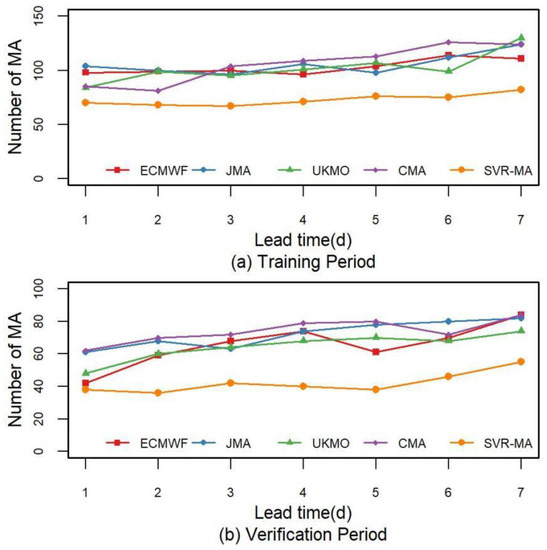
Figure 5.
The number of MAs from the raw NPF and the SVR-MA model in the Meishan Catchment from May to September 2015–2019, where (a) represents the training period (2015–2017) and (b) represents the verification period (2018–2019).
Additionally, the distributions of MA errors from different forecast centers and the SVR-MA model from 2015–2019 are compared in the Meishan Catchment. The results in Figure 6 show the MA error from the different centers and the SVR-MA model in the training period. Figure 6 shows that the MA error from the SVR-MA model has smaller values and fewer outliers. Similar to the results in Figure 6, Figure 7 also shows that the SVR-MA model effectively reduces the MA error. Although the range of boxes for the SVR-MA model during the verification period becomes wider, especially for lead times over 5 d, fewer outlier points still indicate that the method has good control over MA errors.
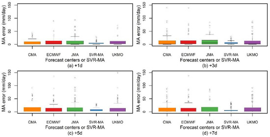
Figure 6.
Box and whisker plots showing the performance in terms of the MA error for different lead times from different centers and the SVR-MA model during the training period. (a) +1d. (b) +3d. (c) +5d. (d) +7d. The horizontal line in the box represents the median of the distribution (50% of the data are greater than this value), and the upper and lower box limits represent the upper and lower quartiles (25% of data greater/lower than the value), respectively. Maximum and minimum values are indicated by the top and bottom horizontal lines. The outlier points show values of more than two-thirds of the quantile.
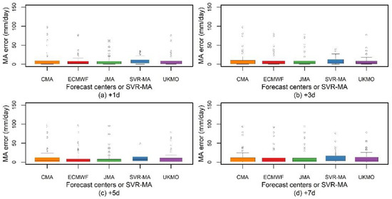
Figure 7.
Box and whisker plots showing the performance in terms of the MA error for different lead times from different centers and the SVR-MA model during the verification period. (a) +1d. (b) +3d. (c) +5d. (d) +7d. The horizontal line in the box represents the median of the distribution (50% of the data are greater than this value), and the upper and lower box limits represent the upper and lower quartiles (25% of data greater/lower than the value), respectively. Maximum and minimum values are indicated by the top and bottom horizontal lines. The outlier points show values of more than two-thirds of the quantile.
3.2. Comparison of Probabilistic Postprocessing Models
Probabilistic postprocessing models are commonly used in flood forecasting and can provide more information about predicted events. However, unlike other hydrological variables, such as runoff, natural precipitation is considered to have a mixed distribution, which makes its conditional distribution more complicated. In this study, two different probabilistic postprocessing models are employed for uncertainty analysis and probabilistic forecasting.
The data from the flood seasons of 2015–2017 are used to determine the distributions and their parameters, and the data from 2018–2019 are used as verification data. All the parameters in the distributions used in this study are estimated by the maximum likelihood estimation, and the distributions are selected by the K-S test. To examine the performance of probabilistic postprocessing models, the RMSEP, Brier score and WPI are selected to evaluate the performance of the two methods. According to Figure 8, the RMSEPs of the two models are quite close, which means they have a similar accuracy. The sharpness of the models is assessed by the WPI in Figure 9. The WPI of the GBM is much smaller than that of the BPM. Additionally, the WPI of the BPM is almost twice that of the GBM when the lead time is over 5 d. Figure 10 shows the Brier score of the two models based on the precipitation forecasts from different centers. The Brier score of the GBM is lower than that of the BPM (Figure 10). As it is a negative indicator, a lower Brier score indicates a better forecast skill in terms of reliability and resolution ability. Figure 8, Figure 9 and Figure 10 show that although the accuracies of the two models are similar in the Meishan Catchment, the probabilistic results from the GBM have a smaller Brier score and WPI, which means that the GBM can improve the sharpness and reliability of probabilistic precipitation forecasts without reducing their accuracy. Additionally, all the three indicators show a trend of deterioration with the growth of the lead time, which may be caused by the increase in variance of raw NPF.
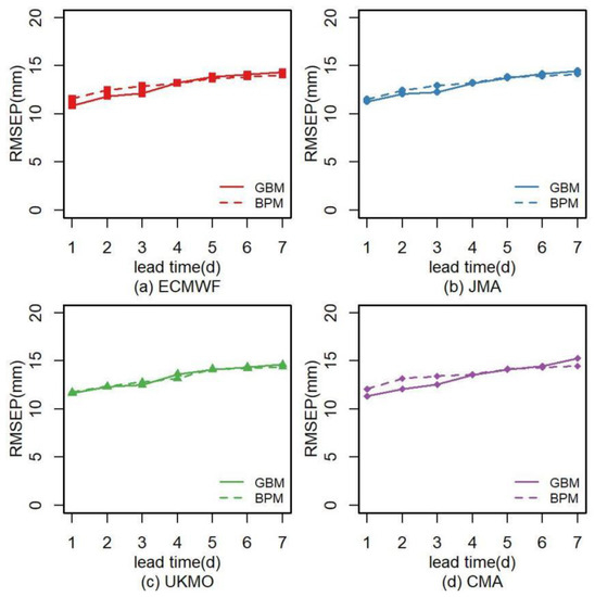
Figure 8.
The RMSEP of the GBM and BPM from different agencies during the verification period over the Meishan Catchment. (a) ECMWF. (b) JMA. (c) UKMO. (d) CMA.
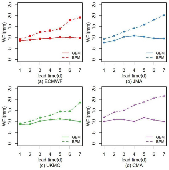
Figure 9.
The WPI of the GBM and BPM from different agencies during the verification period over the Meishan Catchment. (a) ECMWF. (b) JMA. (c) UKMO. (d) CMA.
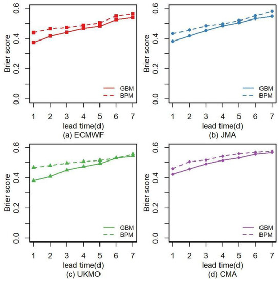
Figure 10.
The Brier scores of the GBM and BPM from different agencies during the verification period over the Meishan Catchment. (a) ECMWF. (b) JMA. (c) UKMO. (d) CMA.
In addition to the improvement in sharpness, reliability, and resolution ability, another advantage of the GBM is that it requires no variable transformation. As a commonly used variable transformation method, NQT is one of the core steps in the BPM, which offers a convenient analytic form for the bivariate density, regardless of the forms of their marginal distributions [52]. However, using NQT will inevitably lead to the transformation of non-normal variables into normal space, which may have impacts on the accuracy of the estimated probability, whereas the GBM can generate the conditional distribution without any variable transformation [53]. Meanwhile, the BPM has a limitation in updating new samples. Since the BPM estimates the marginal distribution of precipitation and precipitation forecasts separately, and builds a joint distribution using Equation (12), when the system has new samples, it has to re-estimate the two marginal distributions and joint distributions. However, for the GBM, assuming that the prior distribution is stable, only the parameters from the likelihood function need to be updated for the new samples. Therefore, the GBM is more suitable for generating probabilistic forecasts for real-time applications.
Furthermore, as indicated in Figure 8, Figure 9 and Figure 10, the probabilistic precipitation forecasts from the JMA and ECMWF are more skillful than those from the other two centers, which indicates that better inputs may lead to better probabilistic results in the GBM. Therefore, a combined framework that uses precipitation forecasts with high accuracies from the multimodel ensemble method as the inputs for probabilistic models is feasible and can generate better probabilistic forecasts.
3.3. Performance Assessment of the New Hybrid Framework
The results above indicate that the performance of the probabilistic postprocessing method is related to the skill of the raw NPF. Accordingly, we examine a new hybrid framework by combining multimodel ensembles and probabilistic postprocessors in this study to obtain a better probabilistic precipitation forecast. The multimodel ensemble results from the SVR-MA model are selected as the inputs of the GBM and compared to the probabilistic results from the raw NPF.
As shown in Figure 11, the RMSEP of probabilistic precipitation forecasting based on the hybrid two-step framework is lower than that of the probabilistic results obtained by the raw NPF. The WPI of the new combined framework also has a better performance (Figure 12). A lower WPI represents a narrower 90% prediction interval, indicating better sharpness. The probabilistic results of the new hybrid framework show a certain advantage in Brier score within 4 d, but this advantage diminishes with increasing lead time (Figure 13). The combined framework has a better performance in all the indicators than the raw NPF, and the advantage is more obvious when the lead time is less than 4 d. Moreover, the results shown in Figure 11, Figure 12 and Figure 13 also support the conclusion that a better probability forecast can be obtained using high-precision raw forecasting. Compared to the best values of the four raw NPF, the RMSEP, WPI, and Brier score from different lead times can be improved by 2–13%, 1–22%, and 0–12% respectively through the hybrid framework, especially for the results with lead times less than 4d, the improvement in accuracy, sharpness, reliability and resolution ability from the hybrid framework can reach 9–13%, 10–22%, and 5–12% respectively.
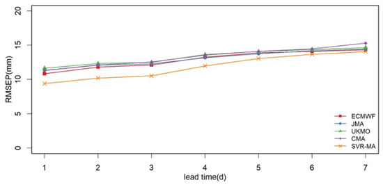
Figure 11.
The RMSEP of the GBM from different inputs (raw NPF of different agencies and the SVR-MA model) during the verification period over the Meishan Catchment.
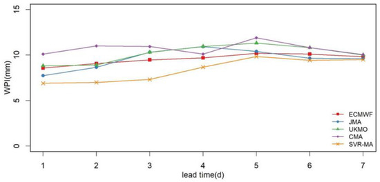
Figure 12.
The WPI of the GBM from different inputs (raw NPF of different agencies and the SVR-MA model) during the verification period over the Meishan Catchment.
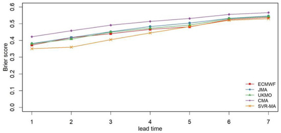
Figure 13.
The Brier score of the GBM from different inputs (raw NPF of different agencies and the SVR-MA model) during the verification period over the Meishan Catchment.
As the main aim of this study is to provide more skillful precipitation forecast to extend the lead time of flood forecast and reservoir regulation, special attention should be paid to the precipitation over 25 mm, i.e., heavy rain and above (Table 1). The main reason for using 25 mm as the threshold rather than a larger value in this study is the number of samples. Figure 14 shows the Brier score of different inputs for observed precipitation over 25 mm during the verification period. From Figure 14, it can be found that the probabilistic results from the hybrid framework have smaller Brier score, which indicates that it is feasible to reduce the MA error through SVR-MA and help the GBM better identify the precipitation with a magnitude over heavy rain. However, the Brier scores in Figure 14 are significantly larger than those in Figure 13, indicating that the forecast skill for heavy rain and above are worse than those for smaller magnitudes. Similarly, the performance of the probabilistic forecast is very poor when the lead time exceeds 4 d in Figure 14.
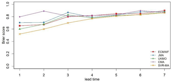
Figure 14.
The Brier score of the GBM from different inputs (raw NPF of different agencies and the SVR-MA model) for precipitation over 25 mm during the verification period over the Meishan Catchment.
In summary, compared to the original NPF, the multimodel ensemble method, SVR-MA, can improve the performance of precipitation forecasting in the Meishan Catchment, especially in terms of reducing MA errors. However, since the accuracy of the inputs (i.e., raw NPFs) decrease with increasing lead time, the correction effect of the SVR-MA method gradually declines, and the MA error is still quite large when the lead time is over 3 d. The forecast skills of probabilistic postprocessors are also evaluated in terms of accuracy, sharpness, reliability, and resolution ability. With its similar RMSEP value, smaller WPI value, lower Brier score, updating advantage, and no variable transformation, the GBM has a better performance than the BPM, and the results imply that better quality inputs can produce better probabilistic forecasts through the GBM. Therefore, a new hybrid framework is proposed by combining the SVR-MA and GBM. The new framework shows an improvement in all the indicators (RMSEP, WPI, and Brier score), especially for lead times lower than 4 d and precipitation over 25 mm. However, the advantages of the new framework also decrease with increasing lead time, which is consistent with changes in the accuracy of the input. The results indicate that the two-step hybrid framework can provide better probabilistic precipitation forecasts. Furthermore, it is worth noticing that only SVR-MA is selected as the multimodel ensemble methods in this paper, but it can be found from the probabilistic results of raw NPF and hybrid two-step framework that all the multimodel ensemble methods which can improve the forecast skill of raw NPF should be applicable to the hybrid two-step framework, and the researchers can flexibly select methods according to their own needs.
3.4. Limitation and Future Work
To improve the skill of precipitation forecast, a new hybrid framework is proposed with combined postprocessors in this study. Certainly, as with all scientific research, this study has several obvious limitations. First, since the measured precipitation from ground stations are used as the “true value” in this study, the study area and time period of this paper are quite limited. The hybrid two-step framework may achieve a better performance based on a larger dataset such as the reanalysis data or satellite products. Moreover, the Thiessen polygon method is employed to calculate the area-average value for observed and forecasted precipitation, and the location and timing errors of precipitation are not considered, which makes the experiment in this study inappropriate for some large basins. Furthermore, since the meteorological system is highly uncertain, the time step used in this paper is limited to daily, which is unfavorable for flash flood forecasting. Another main limitation of this study is that the aim of the hybrid framework is to improve the skill of precipitation forecast for flood forecasting and reservoir regulation, but this paper does not employ the results from the hybrid framework as the input of hydrological models to evaluate the impact of the framework on the performance of actual streamflow forecasting. Finally, although the new hybrid framework shows the potential to improve the skills of precipitation probability forecasting, there is still a lot of room for improvement in practical application to extend the lead time of flood forecast and reservoir regulation.
With the development of meteorological science, more global precipitation forecast datasets based on different meteorological models and initial fields can be used to obtain higher quality multimodel ensemble forecasts. It is possible to obtain precipitation forecasts with higher accuracy, shorter time step, and longer lead time through the hybrid framework and use it as the input of hydrological models for flood forecasting in the future. Meanwhile, the perturbed forecasts from TIGGE have been commonly employed in ensemble forecast, and are also applicable to the hybrid framework of this study. More efforts are still needed to evaluate the performance of the hybrid framework based on the perturbed forecasts in the future. The rapid development of computer science brings a variety of machine learning models for regression and the performance assessment of ensemble forecasts based on different regression models and data sources is also an important task in the future studies. In addition, the errors from location and timing shifts should be taken into consideration in future work to make the framework better adapt to the larger basins.
4. Conclusions
Streamflow forecasting based on hydrological models with an effective lead time is essential for streamflow forecasting and flood control. Although numerical weather forecasting can be used to extend the lead time of hydrologic predictions, its potential in flood forecasting and reservoir regulation has not been fully realized due to the limited accuracy. It is still urgent to reduce the errors in NPFs, especially MA errors, and describe their uncertainty. The main aim of this study is to improve the performance of probabilistic precipitation forecasting based on a new hybrid framework by combining the multimodel ensemble method and probabilistic model. In this study, we employ three different postprocessing methods to reduce errors in NPFs. A multimodel ensemble method, called the SVR-MA, is used to correct the precipitation forecasts, especially with respect to MA errors. In addition, two different probabilistic postprocessors, the BPM and GBM, are employed to analyze uncertainty and compare different aspects. According to the above results, a new combined framework is proposed based on the multimodel ensemble method and the probabilistic forecast method and compared with the probabilistic results from raw NPFs.
Most measurements show that the JMA outperforms other models in the Meishan Catchment, especially when the lead time is shorter than 3 d. The forecast skill of the ECMWF is close to that of the UKMO in forecasts with short lead times (within 3 d), while the ECMWF tends to perform better at a longer lead time. The predictive error of CMA is noticeably larger than that of the other models. In general, the performance of all raw NPFs declines with increasing lead time. Compared to the raw NPF, the SVR-MA method has a slightly lower overall error, but the RMSE-MA and number of Mas sharply decrease, which means that the method has a good ability to control MA errors. However, the correction ability of the SVR-MA method is still gradually affected by the forecast accuracy. When the lead time exceeds 3 d, there are still some MA errors that cannot be corrected by the SVR-MA method due to the limited accuracy of the inputs. Two different probabilistic postprocessing methods are also examined and compared. From the aspects of accuracy, sharpness, reliability, and resolution ability, the GBM shows a better performance than the BPM. Meanwhile, the GBM is not only easier to update with new samples, but also does not need variable transformation, while the NQT in the BPM may lead to a loss of accuracy. Therefore, in this study, the GBM is used as the probabilistic postprocessor of the hybrid two-step framework.
The assessment results show that with the new hybrid framework, all three indicators used in this study are improved. In general, the new framework can provide a probabilistic precipitation forecast with a higher accuracy, better reliability and resolution ability, and smaller confidence intervals, especially when the lead time is below 4 d. Moreover, when the actual precipitation is over 25 mm, the probabilistic forecast from the hybrid framework is more advantageous than others. Moreover, the research also indicates that the performance of probabilistic forecasts is related to the accuracy of their inputs. Therefore, it is possible to obtain a more accurate probability prediction if further improvements of inputs from precipitation forecasting are available by using a multimodel ensemble or other methods. Although the hybrid framework proposed in this paper can improve the skill of precipitation forecast, further efforts are still needed to make its performance meet the demand of practical applications.
Author Contributions
C.C.: writing—original draft, methodology, software. J.W. (Jianqun Wang): conceptualization, funding acquisition, review and editing. Z.L.: supervision, review, and editing. X.S.: review and editing. J.W. (Jinhua Wen) and H.W.: data curation and editing. C.W.: investigation and data curation. All authors have read and agreed to the published version of the manuscript.
Funding
This study is supported by The National Key Research and Development Program of China (grant number: 2016YFC0400909), the China Scholarship Council (No. 201906710062), Applied Basic Public Research Program and Natural Science Foundation of Zhejiang Province (No. LGF22E090007) and Soft Science and Technology Plan Project of Zhejiang Province (No. 2022C35022).
Institutional Review Board Statement
Not applicable.
Informed Consent Statement
Not applicable.
Data Availability Statement
The TIGGE datasets can be downloaded at https://www.ecmwf.int/ (accessed on 1 January 2010). The LIBSVM software can be downloaded at http://www.csie.ntu.edu.tw/~cjlin/libsvm (accessed on 14 April 2021).
Acknowledgments
This study benefited from the TIGGE dataset provided by European Center for Medium-Range Weather Forecasts (ECMWF), Reading, UK. The authors thank Emmanouil Anagnostou for his useful suggestions. The authors are also grateful to the reviewers of the manuscript for their constructive comments and useful suggestions.
Conflicts of Interest
The authors declare no conflict of interest.
Appendix A. Support Vector Regression
The basic idea of an SVR is to convert a nonlinear case to a linear problem by mapping the original problem to a high-dimensional feature space. Let denote the input vector, denote the output vector and the sample set be :
In Equation (A1), is the regression output, represents the nonlinear transformation function, w is the weight vector, and b is the threshold. Then, an ε-SVR model is built by solving the optimization problem:
where C is a cost constant, are the relaxation variables, and is a positive constant, which represents the margin of tolerance.
The dual form of Equation (A2) can be expressed as:
where is the kernel function, while and are Lagrange multipliers. In this study, the radial basis function kernel with an undetermined parameter is employed (Equation (A4)).
In the ε-SVR model, it is necessary to determine ε in advance, but in most practical cases, the value of ε remains unknown before training. Therefore, an alternative parameter, ν, introduced by Schölkopf, has been used in SVR (ν-SVR). The new parameter can not only control the number of support vectors, but also automatically estimate ε, which simplifies the parameter selection (Equation (A5)).
Additionally, the dual form is
Once the three parameters, C, , and ν, are determined, the ν-SVR is established by solving the linear optimization problem in Equation (A6).
References
- Han, H.; Zhao, L. Chinese agricultural water resource utilization: Problems and challenges. Water Policy 2007, 9, 11–28. [Google Scholar]
- Jiang, T.; Su, B.; Huang, J.; Zhai, J.; Xia, J.; Tao, H.; Wang, Y.; Sun, H.; Luo, Y.; Zhang, L.; et al. Each 0.5 °C of warming increases annual flood losses in China by more than 60 billion USD. Bull. Am. Meteorol. Soc. 2020, 101, E1464–E1474. [Google Scholar] [CrossRef]
- Dong, N.; Yang, M.; Yu, Z.; Wei, J.; Yang, C.; Yang, Q.; Liu, X.; Lei, X.; Wang, H.; Kunstmann, H. Water resources management in a reservoir-regulated basin: Implications of reservoir network layout on streamflow and hydrologic alteration. J. Hydrol. 2020, 586, 124903. [Google Scholar] [CrossRef]
- Bao, H.J.; Zhao, L.N.; He, Y.; Li, Z.J.; Wetterhall, F.; Cloke, H.L.; Pappenberger, F.; Manful, D. Coupling ensemble weather predictions based on TIGGE database with Grid-Xinanjiang model for flood forecast. Adv. Geosci. 2011, 29, 61–67. [Google Scholar] [CrossRef]
- Alfieri, L.; Cohen, S.; Galantowicz, J.; Schumann, G.J.; Trigg, M.A.; Zsoter, E.; Prudhomme, C.; Kruczkiewicz, A.; Coughlan De Perez, E.; Flamig, Z.; et al. A global network for operational flood risk reduction. Environ. Sci. Policy 2018, 84, 149–158. [Google Scholar] [CrossRef]
- Ye, J.; Shao, Y.; Li, Z. Flood Forecasting Based on TIGGE Precipitation Ensemble Forecast. Adv. Meteorol. 2016, 2016, 9129734. [Google Scholar] [CrossRef]
- Todini, E. Flood Forecasting and Decision Making in the new Millennium. Where are We? Water Resour. Manag. 2017, 31, 3111–3129. [Google Scholar] [CrossRef]
- Demeritt, D.; Nobert, S.; Cloke, H.L.; Pappenberger, F. The European Flood Alert System and the communication, perception, and use of ensemble predictions for operational flood risk management. Hydrol. Process. 2013, 27, 147–157. [Google Scholar] [CrossRef]
- Hua, L.; Wan, X.; Wang, X.; Zhao, F.; Zhong, P.A.; Liu, M.; Yang, Q. Floodwater Utilization Based on Reservoir Pre-Release Strategy Considering the Worst-Case Scenario. Water 2020, 12, 892. [Google Scholar] [CrossRef]
- Su, X.; Yuan, H.; Zhu, Y.; Luo, Y.; Wang, Y. Evaluation of TIGGE ensemble predictions of Northern Hemisphere summer precipitation during 2008–2012. J. Geophys. Res. Atmos. 2014, 119, 7292–7310. [Google Scholar] [CrossRef]
- Ran, Q.; Fu, W.; Liu, Y.; Li, T.; Shi, K.; Sivakumar, B. Evaluation of Quantitative Precipitation Predictions by ECMWF, CMA, and UKMO for Flood Forecasting: Application to Two Basins in China. Nat. Hazards Rev. 2018, 19, 05018003. [Google Scholar] [CrossRef]
- Louvet, S.; Sultan, B.; Janicot, S.; Kamsu-Tamo, P.H.; Ndiaye, O. Evaluation of TIGGE precipitation forecasts over West Africa at intraseasonal timescale. Clim. Dyn. 2016, 47, 31–47. [Google Scholar] [CrossRef]
- Krishnamurti, T.N.; Kishtawal, C.M.; Zhang, Z.; LaRow, T.; Bachiochi, D.; Williford, E.; Gadgil, S.; Surendran, S. Multimodel Ensemble Forecasts for Weather and Seasonal Climate. J. Clim. 2000, 13, 4196–4216. [Google Scholar] [CrossRef]
- Li, W.; Duan, Q.; Miao, C.; Ye, A.; Gong, W.; Di, Z. A review on statistical postprocessing methods for hydrometeorological ensemble forecasting. Wiley Interdiscip. Rev. Water 2017, 4, e1246. [Google Scholar] [CrossRef]
- Kipkogei, O.; Bhardwaj, A.; Kumar, V.; Ogallo, L.A.; Opijah, F.J.; Mutemi, J.N.; Krishnamurti, T.N. Improving multimodel medium range forecasts over the Greater Horn of Africa using the FSU superensemble. Meteorol. Atmos. Phys. 2016, 128, 441–451. [Google Scholar] [CrossRef]
- Zhi, X.; Qi, H.; Bai, Y.; Lin, C. A Comparison of Three Kinds of Multimodel Ensemble Forecast Techniques Based on the TIGGE Data. Acta Meteorol. Sin. 2012, 26, 41–51. [Google Scholar] [CrossRef]
- Vuillaume, J.; Herath, S. Improving global rainfall forecasting with a weather type approach in Japan. Hydrol. Sci. J. 2017, 62, 167–181. [Google Scholar] [CrossRef]
- Feng, C.; Cui, M.; Hodge, B.; Zhang, J. A data-driven multi-model methodology with deep feature selection for short-term wind forecasting. Appl. Energy 2017, 190, 1245–1257. [Google Scholar] [CrossRef]
- He, Y.; Wetterhall, F.; Cloke, H.L.; Pappenberger, F.; Wilson, M.; Freer, J.; McGregor, G. Tracking the uncertainty in flood alerts driven by grand ensemble weather predictions. Meteorol. Appl. 2009, 16, 91–101. [Google Scholar] [CrossRef]
- Cuo, L.; Pagano, T.C.; Wang, Q.J. A Review of Quantitative Precipitation Forecasts and Their Use in Short- to Medium-Range Streamflow Forecasting. J. Hydrometeorol. 2011, 12, 713–728. [Google Scholar] [CrossRef]
- Jha, S.K.; Shrestha, D.L.; Stadnyk, T.A.; Coulibaly, P. Evaluation of ensemble precipitation forecasts generated through post-processing in a Canadian catchment. Hydrol. Earth Syst. Sci. 2018, 22, 1957–1969. [Google Scholar] [CrossRef]
- Krzysztofowicz, R.; Kelly, K.S. Hydrologic uncertainty processor for probabilistic river stage forecasting. Water Resour. Res. 2000, 36, 3265–3277. [Google Scholar] [CrossRef]
- Herr, H.D.; Krzysztofowicz, R. Generic probability distribution of rainfall in space: The bivariate model. J. Hydrol. 2005, 306, 234–263. [Google Scholar] [CrossRef]
- Robertson, D.E.; Shrestha, D.L.; Wang, Q.J. Post-processing rainfall forecasts from numerical weather prediction models for short-term streamflow forecasting. Hydrol. Earth Syst. Sci. 2013, 17, 3587–3603. [Google Scholar] [CrossRef]
- Wang, Q.J.; Robertson, D.E. Multisite probabilistic forecasting of seasonal flows for streams with zero value occurrences. Water Resour. Res. 2011, 47, W02546. [Google Scholar] [CrossRef]
- Tao, Y.; Duan, Q.; Ye, A.; Gong, W.; Di, Z.; Xiao, M.; Hsu, K. An evaluation of post-processed TIGGE multimodel ensemble precipitation forecast in the Huai river basin. J. Hydrol. 2014, 519, 2890–2905. [Google Scholar] [CrossRef]
- Chen, K.; Yu, J. Short-term wind speed prediction using an unscented kalman filter based state-space support vector regression approach. Appl. Energy 2014, 113, 690–705. [Google Scholar] [CrossRef]
- Ghorbani, M.A.; Khatibi, R.; FazeliFard, M.H.; Naghipour, L.; Makarynskyy, O. Short-term wind speed predictions with machine learning techniques. Meteorol. Atmos. Phys. 2016, 128, 57–72. [Google Scholar] [CrossRef]
- Cai, C.; Wang, J.; Li, Z. Improving TIGGE Precipitation Forecasts Using an SVR Ensemble Approach in the Huaihe River Basin. Adv. Meteorol. 2018, 2018, 7809302. [Google Scholar] [CrossRef]
- Cai, C.; Wang, J.; Li, Z. Assessment and modelling of uncertainty in precipitation forecasts from TIGGE using fuzzy probability and Bayesian theory. J. Hydrol. 2019, 577, 123995. [Google Scholar] [CrossRef]
- Qu, B.; Zhang, X.; Pappenberger, F.; Zhang, T.; Fang, Y. Multi-Model Grand Ensemble Hydrologic Forecasting in the Fu River Basin Using Bayesian Model Averaging. Water 2017, 9, 74. [Google Scholar] [CrossRef]
- Ferro, C.A.T. Comparing Probabilistic Forecasting Systems with the Brier Score. Weather Forecast. 2007, 22, 1076–1088. [Google Scholar] [CrossRef]
- Candille, G.; Talagrand, O. Evaluation of probabilistic prediction systems for a scalar variable. Q. J. R. Meteorol. Soc. 2005, 131, 2131–2150. [Google Scholar] [CrossRef]
- Krishnamurti, T.N.; Kishtawal, C.M.; LaRow, T.E.; Bachiochi, D.R.; Zhang, Z.; Williford, C.E.; Gadgil, S.; Surendran, S. Improved Weather and Seasonal Climate Forecasts from Multimodel Superensemble. Science 1999, 285, 1548–1550. [Google Scholar] [CrossRef] [PubMed]
- Mishra, A.K.; Krishnamurti, T.N. Current status of multimodel superensemble and operational NWP forecast of the Indian summer monsoon. J. Earth Syst. Sci. 2007, 116, 369–384. [Google Scholar] [CrossRef]
- Dibike, Y.B.; Velickov, S.; Solomatine, D.; Abbott, M.B. Model induction with support vector machines: Introduction and applications. J. Comput. Civ. Eng. 2001, 15, 208–216. [Google Scholar] [CrossRef]
- Lin, G.; Chou, Y.; Wu, M. Typhoon flood forecasting using integrated two-stage Support Vector Machine approach. J. Hydrol. 2013, 486, 334–342. [Google Scholar] [CrossRef]
- Yu, P.; Chen, S.; Chang, I. Support vector regression for real-time flood stage forecasting. J. Hydrol. 2006, 328, 704–716. [Google Scholar] [CrossRef]
- Scholkopf, B.; Mika, S.; Burges, C.J.C.; Knirsch, P.; Muller, K.; Ratsch, G.; Smola, A.J. Input Space Versus Feature Space in Kernel-Based Methods. Ieee Trans. Neural Netw. 1999, 10, 1000–1017. [Google Scholar] [CrossRef]
- Chang, C.; Lin, C. LIBSVM: A Library for Support Vector Machines. ACM Trans. Intell. Syst. Technol. 2011, 2, 1–27. [Google Scholar] [CrossRef]
- Wu, L.; Seo, D.; Demargne, J.; Brown, J.D.; Cong, S.; Schaake, J. Generation of ensemble precipitation forecast from single-valued quantitative precipitation forecast for hydrologic ensemble prediction. J. Hydrol. 2011, 399, 281–298. [Google Scholar] [CrossRef]
- Liu, B.; Chen, X.; Lian, Y.; Wu, L. Entropy-based assessment and zoning of rainfall distribution. J. Hydrol. 2013, 490, 32–40. [Google Scholar] [CrossRef]
- Papalexiou, S.M.; Koutsoyiannis, D. A global survey on the seasonal variation of the marginal distribution of daily precipitation. Adv. Water Resour. 2016, 94, 131–145. [Google Scholar] [CrossRef]
- Demargne, J.; Wu, L.; Regonda, S.K.; Brown, J.D.; Lee, H.; He, M.; Seo, D.; Hartman, R.; Herr, H.D.; Fresch, M.; et al. The Science of NOAA′s Operational Hydrologic Ensemble Forecast Service. Bull. Am. Meteorol. Soc. 2014, 95, 79–98. [Google Scholar] [CrossRef]
- Browna, J.D.; Wu, L.; He, M.; Regonda, S.; Lee, H.; Seo, D. Verification of temperature, precipitation, and streamflow forecasts from the NOAA/NWS Hydrologic Ensemble Forecast Service (HEFS): 1. Experimental design and forcing verification. J. Hydrol. 2014, 519, 2869–2889. [Google Scholar] [CrossRef]
- Zhang, Y.; Wu, L.; Scheuerer, M.; Schaake, J.; Kongoli, C. Comparison of Probabilistic Quantitative Precipitation Forecasts from Two Postprocessing Mechanisms. J. Hydrometeorol. 2017, 18, 2873–2891. [Google Scholar] [CrossRef]
- Ghazvinian, M.; Zhang, Y.; Seo, D.J. A Nonhomogeneous Regression-Based Statistical Postprocessing Scheme for Generating Probabilistic Quantitative Precipitation Forecast. J. Hydrometeorol. 2020, 21, 2275–2291. [Google Scholar] [CrossRef]
- Ghazviniana, M.; Zhang, Y.; Seo, D.; He, M.; Fernando, N. A novel hybrid artificial neural network—Parametric scheme for postprocessing medium-range precipitation forecasts. Adv. Water Resour. 2021, 151, 103907. [Google Scholar] [CrossRef]
- Bardossy, A.; Plate, E.J. Space-time model for daily rainfall using atmospheric circulation patterns. Water Resour. Res. 1992, 28, 1247–1259. [Google Scholar] [CrossRef]
- Reggiani, P.; Boyko, O. A Bayesian Processor of Uncertainty for Precipitation Forecasting Using Multiple Predictors and Censoring. Mon. Weather Rev. 2019, 147, 4367–4387. [Google Scholar] [CrossRef]
- Bougeault, P.; Toth, Z.; Bishop, C.; Brown, B.; Burridge, D.; Chen, D.H.; Ebert, B.; Fuentes, M.; Hamill, T.M.; Mylne, K.; et al. The THORPEX Interactive Grand Global Ensemble. Bull. Am. Meteorol. Soc. 2010, 91, 1059–1072. [Google Scholar] [CrossRef]
- Kelly, K.S.; Krzysztofowicz, R. A bivariate meta-Gaussian density for use in hydrology. Stoch. Hydrol. Hydraul. Res. J. 1997, 11, 17–31. [Google Scholar] [CrossRef]
- Khajehei, S.; Moradkhani, H. Towards an improved ensemble precipitation forecast: A probabilistic post-processing approach. J. Hydrol. 2017, 546, 476–489. [Google Scholar] [CrossRef]
Publisher’s Note: MDPI stays neutral with regard to jurisdictional claims in published maps and institutional affiliations. |
© 2022 by the authors. Licensee MDPI, Basel, Switzerland. This article is an open access article distributed under the terms and conditions of the Creative Commons Attribution (CC BY) license (https://creativecommons.org/licenses/by/4.0/).