Evaluation of Five Equations for Short-Term Reference Evapotranspiration Forecasting Using Public Temperature Forecasts for North China Plain

Abstract

Accurate short-term forecasts of daily reference evapotranspiration (ET₀) are essential for real-time irrigation scheduling. Many models rely on current and historical temperature data to estimate daily ET₀. However, easily accessible temperature forecasts are relatively less reported in short-term ET₀ forecasting. Furthermore, the accuracy of ET₀ forecasting from different models varies locally and also across regions. We used five temperature-dependent models to forecast daily ET₀ for a 7-day horizon in the North China Plain (NCP): the McCloud (MC), Hargreaves-Samani (HS), Blaney-Criddle (BC), Thornthwaite (TH), and reduced-set Penman–Monteith (RPM) models. Daily meteorological data collected between 1 January 2000 and 31 December 2014 at 17 weather stations in NCP to calibrate and validate the five ET₀ models against the ASCE Penman–Monteith (ASCE-PM). Forecast temperatures for up to 7 d ahead for 1 January 2015–19 June 2021 were input to the five calibrated models to forecast ET₀. The performance of the five models improved for forecasts at all stations after calibration. The calibrated RPM is the preferred choice for forecasting ET₀ in NCP. In descending order of preference, the remaining models were ranked as HS, TH, BC, and MC. Sensitivity analysis showed that a change in maximum temperature influenced the accuracy of ET₀ forecasting by the five models, especially RPM, HS, and TH, more than other variables. Meanwhile, the calibrated RPM and HS equations were better than the other models, and thus, these two equations were recommended for short-term ET₀ forecasting in NCP.

1. Introduction

The North China Plain (NCP) is China’s most important grain-producing region, and it is facing severe resource constraints such as low carbon and inadequate water conservation [1]. Insufficient usable water resources and fierce competition for industrial and agricultural water have led to the severe overexploitation of groundwater in some areas [2]. Water-saving irrigation techniques and science-based irrigation decisions are important to ensure agricultural water supplies in the NCP [3,4].

Accurate daily reference evapotranspiration (ET₀) forecasts are essential for real-time irrigation demand estimation [5]. The ET₀ models available in the literature can be broadly classified as (1) fully physically based combination models that account for mass and energy conservation principles; (2) black-box models based on artificial neural networks, empirical relationships, and fuzzy and genetic algorithms; and (3) semi-physically based models dealing with either mass or energy conservation [6].

The fully physically based combination models mainly include the Penman–Monteith (ASCE-PM) [7], the Original Penman–Monteith [8], FAO-24 [9], Kimberly Penman [10,11,12], and FAO56 Penman–Monteith [13] models. The ASCE-PM model is recommended as the standard model for estimating ET₀ and as a benchmark to evaluate other models [7,14]. However, the application of ASCE-PM is limited by the lack of required weather variables in many regions. Therefore, under the condition of the deficiency of climatological data, many studies have used machine learning models due to their excellent capability for tackling non-linear relationships between dependent and independent variables [15,16,17].

Many researchers have emphasized ET₀ modeling using machine learning, such as multi-layer perceptron (MLP) [18,19], extreme learning machine (ELM) [20,21], support vector machines (SVMs) [22,23], support vector regression (SVR) [24], and extreme learning machines (ELMs). They have mainly emphasized estimating the current ET₀ using various computing approaches, while less attention has been paid to machine learning codes to forecast futuristic ET₀. The network was performed as a black box with no possibility of providing algebraic equations for rapid deployment. Traore et al. [19] forecasted daily ET₀ based on gene-expression programming (GEP) with the limited public weather forecast in Jiangsu, China, and found that the GEP algorithm is a deployable tool for ET₀ forecasts to anticipate decisions on short-term irrigation scheduling. They proposed a deployable model formulated into mathematic equations. The above methods take fewer variables as input and can produce precise results. However, for farmers and policymakers in rural areas, the machine learning methods are difficult to understand and employ. In addition, the soft computing methods are often not free and require high-performance computers. This makes it difficult to estimate ET₀, particularly in remote areas where most irrigated fields are located, specifically in the developing and emerging world. For this reason, simpler empirical equations that require fewer climatic variables for ET₀ calculation are utilized [25].

There are several simpler temperature-based equations such as Hargreaves, Hargreaves and Samani [26], Thornthwaite [27], and Blaney and Criddle [28], which were developed to be used with weather data. Many recent studies have investigated the feasibility of ET₀ calculation based on forecast temperature. Trajkovic [29] found that a temperature-based radial basis function (RBF) network can be used to forecast ET₀ when relative humidity, radiation, and wind speed data are unavailable. Lu et al. [30] compared three temperature-based estimation models with three radiation-based estimation models and recommended the Hamon model for use in the southeastern United States. The temperature-based Hargreaves–Samani (HS) model has been used to forecast ET₀ in many studies and produced good results [31,32,33,34]. Other models, such as Thornthwaite (TH) and Blaney–Criddle (BC), can also be used to forecast ET₀ after being calibrated [5,35,36,37].

Most of the above studies used current and historical weather data. Farmers and irrigation professionals make their decisions based on day-to-day water-balance estimation. Real-time irrigation demand estimation is challenging. Anticipating irrigation scheduling and water resources planning is a concern. Public weather forecast is easily accessible, and the forecast maximum and minimum temperatures are highly accurate [32,33,38,39]. Such temperature data could be used to accurately calculate and forecast ET₀ and forecast irrigation demand in the near future [19,40]. Luo et al. [41] proposed using a locally calibrated HS model and temperature forecast for short-term ET₀ forecasts and found that the method can provide daily ET₀ forecasts with certain accuracy for real-time irrigation forecast. Xiong et al. [5] forecast ET₀ with the BC model and temperature forecast, and the results indicate that the BC model can be an alternative and effective solution for forecast ET₀ in east China. Chang et al. [35] used a modified daily TH equation and temperature forecasts for ET₀ forecasts and found that TH produced good ET₀ forecast results and can be a feasible solution for short-term ET₀ forecasts. The temperature-based models are simple, convenient, and practical, and they are widely applicable in forecasting ET₀ [38,42]. Although NCP has the greatest rate of agricultural irrigation in China, there has been little research into short-term ET₀ forecasts for NCP. Some studies have limited their interest to one model or investigated models that were impractical for various reasons, so it seems that the real-time irrigation demand and irrigation water requirements forecasting in NCP may benefit from comparative research into five different temperature-based models for short-term ET₀ forecasting. Most extant models require some form of correction for the particular area they are modeling, while the lack of model comparison caused confusion about whether this model is the best one for that region. It is therefore necessary to compare five models to determine the most accurate method for short-term ET₀ forecasts in NCP.

The main objectives of this study were (1) to investigate the accuracy of short-time ET₀ forecasting using five models with the public weather forecasts in NCP, (2) to produce five sets of calibrated parameters for temperature-based ET₀ models and to recommend the best short-term ET₀ model in NCP using the statistical indicators as criteria, and (3) to explore error source and the sensitivity of short-term ET₀ forecasts to the percentage change in temperature forecast.

2. Materials and Methods

2.1. Study Area

The NCP is in the east of China, between 34°46′–40°25′ N and 112°30′–119°30′ E. It includes Beijing, Tianjin, the Hebei plain, the northern Henan plain, and the northern Shandong Plain north of the Yellow River [1]. The NCP is one of the three greatest plains in China. Its population is the largest in China, and it is an important grain-producing area. Agricultural irrigation is vital here. The NCP has a temperate and sub-tropical monsoon climate. It is the core area for economic development in north China, and water shortage is considered a severe threat there [2].

Figure 1 shows the locations of 17 weather stations (WS) in the NCP. Botou (BT), Tangshan (TS), and Xinxiang (XX) stations were selected as representative WS, and the characteristics of the WS are listed in

Table 1. Characteristics of weather stations in the study areas.

No.	WMO No.	Station	Province	Longitude	Latitude	Elevation (m)
1	53,798	Xingtai (XT)	Hebei	114.5° E	37.1° N	77.3
2	54,518	Bazhou (BZ)	Hebei	116.4° E	39.2° N	8.9
3	54,534	Tangshan (TS)	Hebei	118.1° E	39.7° N	23.2
4	54,539	Laoting (LT)	Hebei	118.9° E	39.4° N	8.5
5	54,602	Baoding (BG)	Hebei	115.5° E	38.7° N	16.8
6	54,606	Raoyang (RY)	Hebei	115.7° E	38.2° N	19.0
7	54,618	Botou (BT)	Hebei	116.6° E	38.1° N	13.2
8	54,624	Huanghua (HH)	Hebei	117.3° E	38.4° N	4.5
9	54,705	Nangong (NG)	Hebei	115.4° E	37.4° N	27.4
10	53,986	Xinxiang (XX)	Henan	113.9° E	35.3° N	73.2
11	54,416	Miyun (MY)	Beijing	116.9° E	40.4° N	71.8
12	54,511	Beijing (BJ)	Beijing	116.5° E	39.8° N	31.3
13	54,525	Baodi (BI)	Tianjin	117.3° E	39.7° N	5.1
14	54,527	Tianjin (TJ)	Tianjin	117.1° E	39.1° N	3.5
15	54,715	Lingxian (LX)	Shandong	116.6° E	37.3° N	18.6
16	54,725	Huimin (HM)	Shandong	117.5° E	37.5° N	11.7
17	54,808	Shenxian (SX)	Shandong	115.6° E	36.2° N	37.8

. The latitudes of the WS are between 35.3° and 40.4° N, and the longitudes from 113.8° to 118.9°E, with their elevation ranging from 3.5 m to 77.3 m.

2.2. Data

Meteorological data, including daily minimum and maximum air temperature, average wind speed, average relative humidity, and sunshine duration, were obtained from 17 standard national weather stations (WS) from the China Meteorological Data Network (http://data.cma.gov.cn accessed on 30 June 2021). The 7 d ahead temperature forecast was collected from the China Weather Network (http://www.weather.com.cn accessed on 30 June 2021).

Daily meteorological data recorded from 1 January 2000 to 31 December 2014 at the 17 stations in NCP were used to calibrate and validate the five selected ET₀ temperature-based forecast models against the ASCE Penman–Monteith (ASCE-PM) model. Forecast temperatures up to 7 d ahead for 1 January 2015–19 June 2021 were input to the five calibrated models to forecast ET₀. Data used in the study are shown in

Table 2. Data used in the study.

Data Type	Data	Time Period	Data Source
Meteorological data	Tmax, Tmin, RHmean, SH, U2	1 January 1970–20 June 2021	http://data.cma.gov.cn
Temperature forecast	Tmax, Tmin	1 January 2015–19 June 2021	http://www.weather.com.cn

Note: T_max = daily maximum air temperature; T_min = daily minimum air temperature; RH_mean = average relative humidity; SH = sunshine duration; U₂ = wind speed at 2 m.

.

2.3. Method

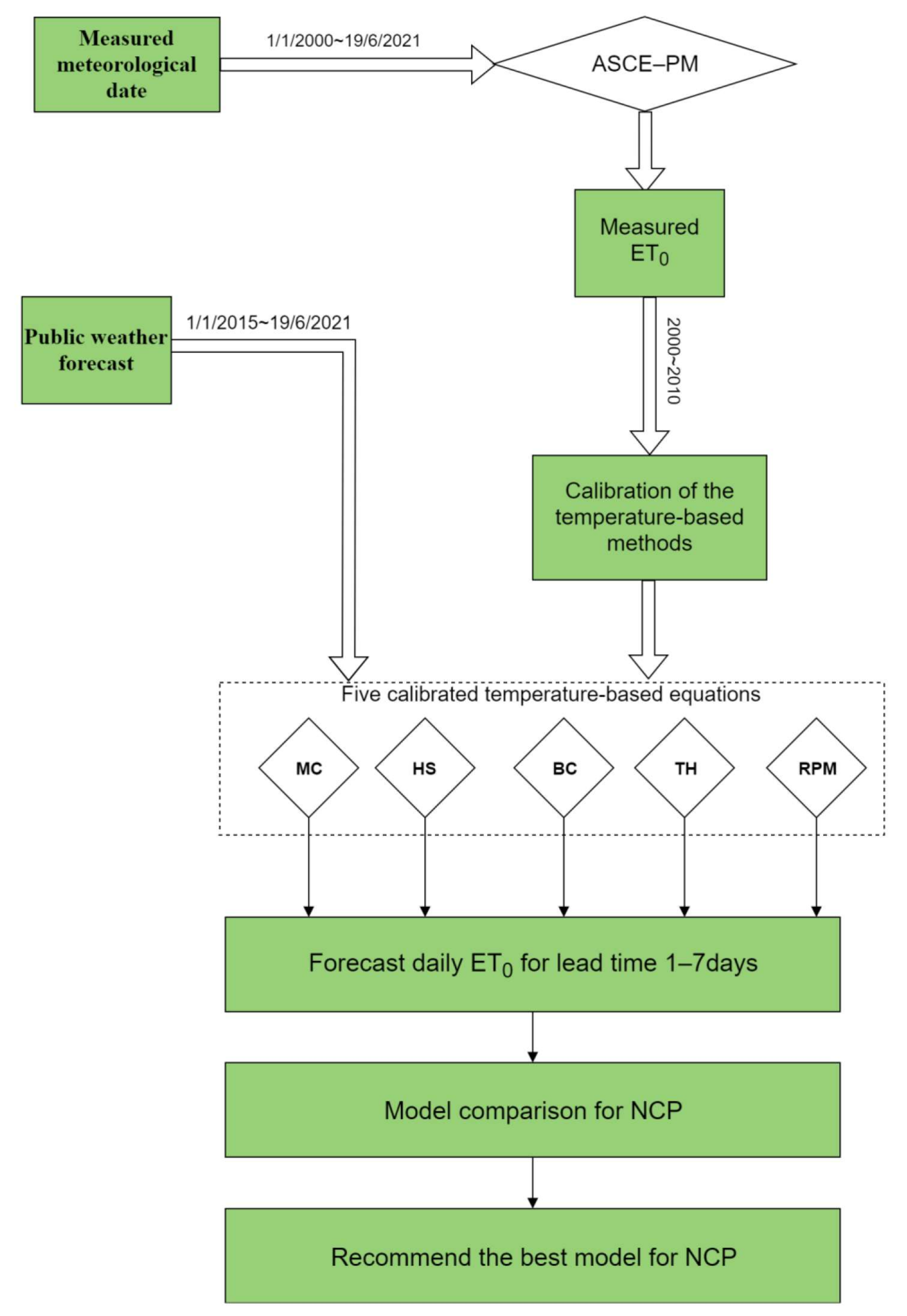
Five air temperature-based models, the McCloud (MC), Thornthwaite (TH), Blaney–Criddle (BC), Hargreaves–Samani (HS), and reduced-set Penman–Monteith (RPM) models, were selected for this study to calculate and forecast local ET₀ [29,31,36,37,38,42,43]. Air-temperature-based models can accurately and reliably forecast daily ET₀ in China [33,34,38,42]. Penman–Monteith (ASCE-PM) [7] has been recommended as the standard model for estimating ET₀ and as a target to evaluate other models [7,14]. However, ASCE-PM requires several meteorological variables as input, and thus it is not practical for areas where the required daily meteorological input data is not available [5,29,36]. Figure 2 shows the workflow of the ET₀ forecast in this study.

2.3.1. ASCE Penman–Monteith Model

The ASCE-Penman–Monteith (ASCE-PM) equation is [7]:

$${\mathrm{ET}}_{0,\mathrm{PM}}=\frac{0.408\mathsf{\Delta }\left({\mathrm{R}}_{\mathrm{n}}-\mathrm{G}\right)+\mathsf{\gamma }\frac{\mathrm{Cn}}{\mathrm{T}+273}{\mathrm{U}}_2\left({\mathrm{e}}_{\mathrm{s}}-{\mathrm{e}}_{\mathrm{a}}\right)}{\mathsf{\Delta }+\mathsf{\gamma }\left(1+{\mathrm{CdU}}_2\right)}$$

(1)

where: ${\mathrm{ET}}_{0,\mathrm{PM}}$ is the daily ET₀ (mm/d) calculated by the ASCE-PM equation; R_n is the net irradiance on the crop surface (MJ/m²/d); G is the soil heat flux density (MJ/m²/d); T is the air temperature at a height of 2 m (°C); U₂ is the wind speed at a height of 2 m (m/s); ${\mathrm{e}}_{\mathrm{s}}$ is the saturated air vapor pressure (kPa); ${\mathrm{e}}_{\mathrm{a}}$ is the measured vapor pressure (kPa); Δ is the slope of the vapor pressure curve (kPa/°C); γ is the psychometric constant (kPa/°C).

If the wind speed at 2 m is not measured, the equation is empirically calculated as a function using measured sunshine and measured wind speed at 10 m [13] as follows:

$${\mathrm{U}}_2={\mathrm{U}}_{\mathrm{z}}\frac{4.87}{\ln \left(67.8\mathrm{z}-5.42\right)}$$

(2)

$${\mathrm{R}}_{\mathrm{s}}=\left({\mathrm{a}}_{\mathrm{s}}+{\mathrm{b}}_{\mathrm{s}}\frac{\mathrm{n}}{\mathrm{N}}\right){\mathrm{R}}_{\mathrm{a}}$$

(3)

where: ${\mathrm{U}}_2$ is the wind speed at 2 m height (m/s); ${\mathrm{U}}_{\mathrm{z}}$ is the measured wind speed at z m height (m/s); z is the measurement height (10 m); ${\mathrm{R}}_{\mathrm{s}}$ is the daily solar or shortwave irradiance (MJ/m²/d); n is the sunshine duration (h); N is the maximum possible duration of sunshine or daylight hours (h); Ra is the extraterrestrial radiation (MJ/m²/d); ${\mathrm{a}}_{\mathrm{s}}$ (0.25) and ${\mathrm{b}}_{\mathrm{s}}$ (0.5) are constants recommended in ASCE-EWRI [7]. Considering that there is short grass around the China Meteorological weather station and that ET₀ was calculated on the daily time scale, the value of Cn and Cd are 900 and 0.34, respectively.

2.3.2. McCloud Model

McCloud [44] developed the McCloud (MC) equation for the ET₀ estimation of land in Florida. The MC equation is:

$${\mathrm{ET}}_{0,\mathrm{MC}}={\mathrm{KW}}^{1.8\mathrm{T}}$$

(4)

where: ${\mathrm{ET}}_{0,\mathrm{MC}}$ is ET₀ calculated by the MC equation (mm/d); K (0.254) and W (1.07) are both recommended default values [42]; T is the daily mean measured air temperature (°C) at a screen height of 2.0 m.

2.3.3. Hargreaves–Samani Model

The Hargreaves–Samani (HS) model [26] for ET₀ estimation is expressed as:

$${\mathrm{ET}}_{0,\mathrm{HS}}=\frac{1}{\mathsf{\lambda }}\mathrm{C}\cdot {\mathrm{R}}_{\mathrm{a}}\cdot {\left({\mathrm{T}}_{\max }-{\mathrm{T}}_{\min }\right)}^{\mathrm{E}}\cdot \left(\frac{{\mathrm{T}}_{\max }+{\mathrm{T}}_{\min }}{2}+\mathrm{T}\right)$$

(5)

where: ${\mathrm{ET}}_{0,\mathrm{HS}}$ is the daily ET₀ calculated by the HS equation (mm/d); ${\mathrm{T}}_{\max }$ and ${\mathrm{T}}_{\min }$ are the maximum and minimum air temperature (°C); Ra is the extraterrestrial irradiance (MJ/m²/d); C (0.0023) and E (0.5) are parameters with recommended values [26,33,34]. The HS model has been widely used in various climates, and many studies have found that the values of the parameters C and E vary from region to region. To ensure model accuracy, the local calibration of these two parameters is necessary [32,34].

2.3.4. Blaney–Criddle Model

Blaney and Criddle [28] developed the BC model to calculate daily ET₀. The equation is:

$${\mathrm{ET}}_{0,\mathrm{BC}}=\mathrm{P}\left(0.46{\mathrm{T}}_{\mathrm{m}}+8.13\right)$$

(6)

where ${\mathrm{ET}}_{0,\mathrm{BC}}$ is the daily ET₀ calculated by the BC model (mm/d), and Tm is the daily mean air temperature (°C) calculated according to daily ${\mathrm{T}}_{\max }$ and ${\mathrm{T}}_{\min }$, as ${\mathrm{T}}_{\mathrm{m}}=\left({\mathrm{T}}_{\max }+{\mathrm{T}}_{\min }\right)/2$. The parameter p is the daily percentage of annual daytime hours (%).

2.3.5. Adjusted Thornthwaite Model

The Thornthwaite (TH) model was developed by Thornthwaite [27], and the adjusted TH model was developed by Pereira and Pruitt [45]. The adjusted TH model to calculate ET₀ is:

$${\mathrm{ET}}_{0,\mathrm{TH}}\left\{\begin{array}{c}0 {\mathrm{T}}_{\mathrm{ef}}<0 ℃\\ 16·\mathrm{C}·{\left(\frac{10·{\mathrm{T}}_{\mathrm{ef}}}{\mathrm{I}}\right)}^{\mathrm{a}} 0 ℃\le {\mathrm{T}}_{\mathrm{ef}}\le 26 ℃\\ \mathrm{C}·\left(-415.85+32.24{\mathrm{T}}_{\mathrm{ef}}-0.43{\mathrm{T}}_{\mathrm{ef}}{}^2\right) {\mathrm{T}}_{\mathrm{ef}}>26 ℃\end{array}\right.$$

(7)

with:

$${\mathrm{T}}_{\mathrm{ef}}=0.5\mathrm{K}\left(3{\mathrm{Tmin}}_{\max }\right)$$

(8)

$$\mathrm{I}={{\displaystyle \sum }}_{\mathrm{i}=1}^{12}{\left(0.2{\mathrm{T}}_{\mathrm{i}}\right)}^{1.514}$$

(9)

$$\mathrm{a}=0.49+0.0179\mathrm{I}-0.0000771{\mathrm{I}}^2+0.000000675{\mathrm{I}}^3$$

(10)

where: ${\mathrm{ET}}_{0,\mathrm{TH}}$ is the daily ET₀ calculated by the Thornthwaite equation (mm/d); I is a thermal index representing the local normal temperature regime; ${\mathrm{T}}_{\mathrm{i}}$ is the monthly average air temperature (°C), 0 if negative; the exponent a is a function of I; ${\mathrm{T}}_{\mathrm{ef}}$ is the effective daily temperature (°C); K is a calibration coefficient with a recommended value of 0.69 for calculating monthly ET₀.

2.3.6. Reduced-Set Penman–Monteith Model

Allen et al. [13] proposed a modified version of the PM equation, the reduced-set Penman–Monteith (RPM) model that uses only T and U values as input data. Solar irradiance ${\mathrm{R}}_{\mathrm{S}}$ in the PM model and actual water vapor pressure ${\mathrm{e}}_a$ are considered to be functions of temperature, and the wind speed at 2 m above the ground is assumed to be constant at 2 m/s because the most accurate RPM model is obtained by using 2 m/s wind speed as the input to the model [46]. The specific equation is:

$${\mathrm{R}}_{\mathrm{s}}=\mathrm{K}{\left({\mathrm{T}}_{\max }-{\mathrm{T}}_{\min }\right)}^{0.5}{\mathrm{R}}_{\mathrm{a}}$$

(11)

$${\mathrm{e}}_{\mathrm{a}}=0.6108\exp \left(\frac{17.27{\mathrm{T}}_{\min }}{{\mathrm{T}}_{\min }}\right)$$

(12)

where: ${\mathrm{R}}_S$ is the solar irradiance (MJ/m²/d); ${\mathrm{R}}_a$ is the extraterrestrial irradiance (MJ/m²/d); ${\mathrm{T}}_{\max }$ and ${\mathrm{T}}_{\min }$ are the maximum and minimum air temperatures (°C); K is an adjustment coefficient: K = 0.16 for inland locations and K = 0.19 for coastal locations; ${\mathrm{e}}_a$ is the actual vapor pressure (kPa). The RPM is used with these values to calculate ET_0,RPM.

2.3.7. Calibration Method

In this study, calibration is the iterative process of comparing the ET₀ by the five temperature-based models with ET_0,P, revising the model if necessary, comparing again, until a model is accepted (validated). Although the HS equation appears to be applicable in any region or climate, its calculation accuracy actually varies according to region, and some studies have found the accuracy increased if C and E are calibrated for regional differences. The least squares method (LSM) is used to calibrate the values of the parameters C and E in the HS equation [29,31,33].

For the calibration of the other four temperature-based ET₀ models (MC, BC, RPM, and TH), ET₀ calculated by the ASCE-PM model (ET_0,P) is considered to be the ground truth, and linear regression between ET_0,P and ET₀ calculated by the other models was used to correct the models for regional calibration. The linear regression model was:

$${\mathrm{ET}}_{0,\mathrm{P}}={\mathrm{bET}}_{0,\mathrm{T}}+\mathrm{a}$$

(13)

where ${\mathrm{ET}}_{0,\mathrm{P}}$ is the ET₀ calculated by ASCE-PM (mm/d); ${\mathrm{ET}}_{0,\mathrm{T}}$ is the ET₀ estimated by the temperature-based models (mm/d); a and b are the correlation coefficients.

2.3.8. Statistical Analysis

We used several statistical indicators to test the correctness of the temperature-dependent models against the calculations of the ASCE-PM model. The indicators include accuracy (Acc), which is defined as the number of days in which the absolute errors of minimum and maximum temperature calculations are within ±2 °C as a percentage of the total number of samples [5,47]. The accuracy of ET₀ forecasting was similarly defined as the number of days in which the absolute error of forecast ET₀ was within ±1.5 mm/d as a percentage of the total number of samples [5]. Mean absolute error (MAE), root mean square error (RMSE), and the correlation coefficient (R) were also used for comparisons [5,41,42,46]. The equations for these indicators are:

$$\mathrm{Acc}=\frac{{\mathrm{N}}_{\mathrm{rK}}}{{\mathrm{N}}_{\mathrm{fK}}}\times 100\%$$

(14)

$$\mathrm{MAE}=\frac{{{\displaystyle \sum }}_{\mathrm{i}=1}^{\mathrm{n}}\left|{\mathrm{E}}_{\mathrm{Ti}}-{\mathrm{E}}_{\mathrm{i}}\right|}{\mathrm{n}}$$

(15)

$$\mathrm{RMSE}=\sqrt{\frac{{{\displaystyle \sum }}_{\mathrm{i}=1}^{\mathrm{n}}{\left({\mathrm{E}}_{\mathrm{Ti}}-{\mathrm{E}}_{\mathrm{i}}\right)}^2}{\mathrm{n}}}$$

(16)

$$\mathrm{R}=\frac{{{\displaystyle \sum }}_{\mathrm{i}=1}^{\mathrm{n}}\left({\mathrm{E}}_{\mathrm{Ti}}-\overline{{\mathrm{E}}_{\mathrm{T}}}\right)\left({\mathrm{E}}_{\mathrm{i}}-\overline{\mathrm{E}}\right)}{\sqrt{{{\displaystyle \sum }}_{\mathrm{i}=1}^{\mathrm{n}}{\left({\mathrm{E}}_{\mathrm{Ti}}-\overline{{\mathrm{E}}_{\mathrm{T}}}\right)}^2·{{\displaystyle \sum }}_{\mathrm{i}=1}^{\mathrm{n}}{\left({\mathrm{E}}_{\mathrm{i}}-\overline{\mathrm{E}}\right)}^2}}$$

(17)

where: ${\mathrm{E}}_{\mathrm{Ti}}$ is the forecast temperature or the forecast ET₀; ${\mathrm{E}}_{\mathrm{i}}$ is the measured air temperature or the calculated ET₀ with the measured meteorological data based on ASCE-PM; i is the calculated sample ordinal number, I = 1, 2, 3…n; N is the total number of samples; $\overline{{\mathrm{E}}_{\mathrm{T}}}$ is the mean value of the calculated sequence, and $\overline{\mathrm{E}}$ is the mean value of the calculated sequence; K is T or E and is the error range for $\left|{\mathrm{E}}_{\mathrm{Ti}}-{\mathrm{E}}_{\mathrm{i}}\right|\le 2 °\mathrm{C}$ and $\left|{\mathrm{E}}_{\mathrm{Ti}}-{\mathrm{E}}_{\mathrm{i}}\right|\le 1.5 \mathrm{mm}/\mathrm{d}$; ${\mathrm{N}}_{\mathrm{rK}}$ is the number of days for which the forecasting is correct; ${\mathrm{N}}_{\mathrm{fK}}$ is the total number of days forecast.

3. Results and Discussion

3.1. Evaluation of Temperature Forecasts

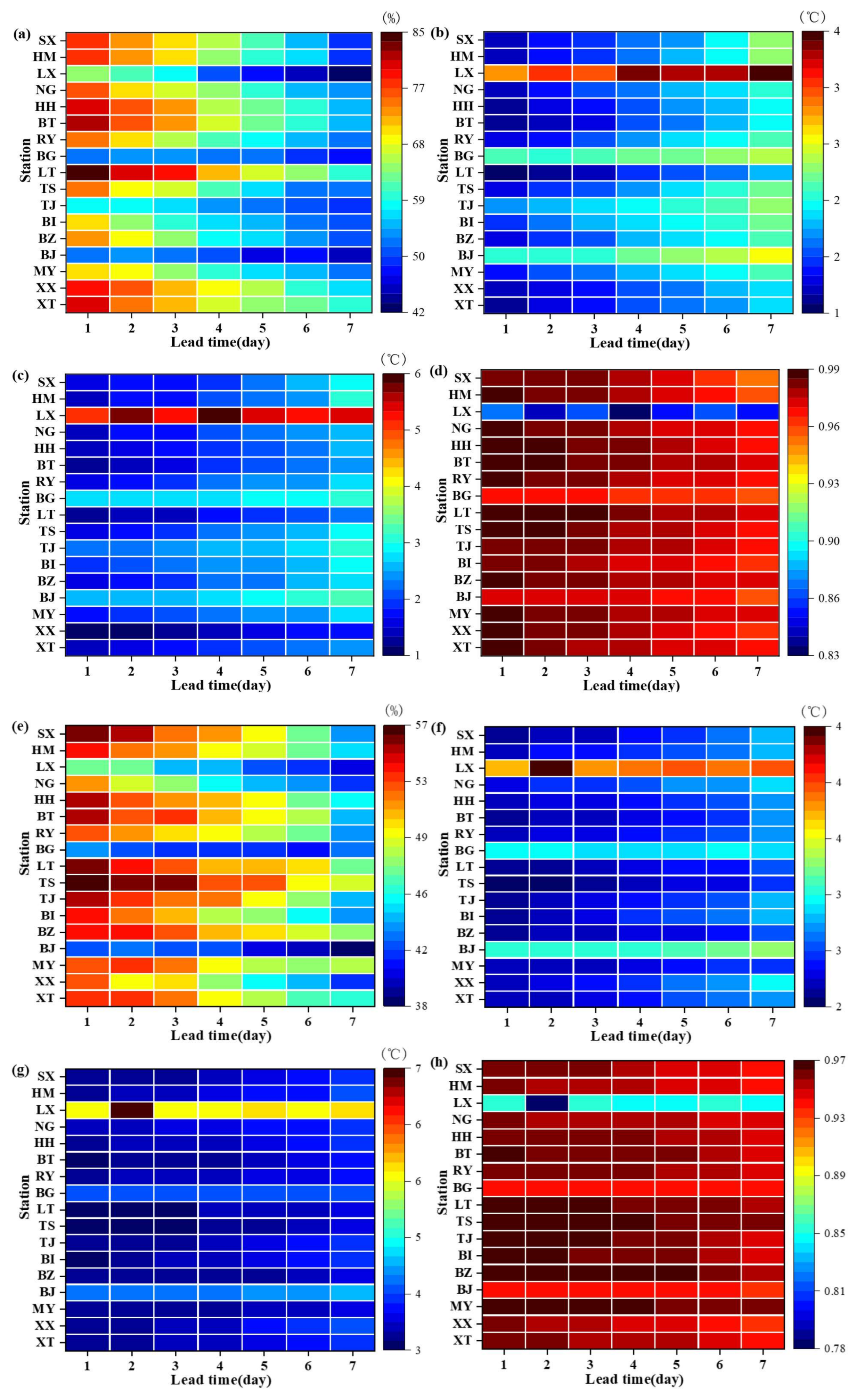
A temperature-based ET₀ model uses air temperature data as input to calculate ET₀, so the accuracy of the air temperature forecast affects the accuracy of the ET₀ forecast. We used Acc, MAE, RMSE, and R to evaluate the accuracy of the minimum and maximum temperature forecasts for the 17 WS in NCP. The values of the statistical indicators are shown in Figure 3. For all stations, the range of Acc for T_min for 1 d ahead was 52–85% and for 7 d ahead was 42–60%. The corresponding ranges for R were 0.87–0.99 and 0.86–0.97, respectively. MAE and RMSE for ${\mathrm{T}}_{\min }$ were the least for the 1 d ahead and the greatest for 7 d ahead. The range of Acc for ${\mathrm{T}}_{\max }$ for 1 d ahead was 42.36–56.54% and for 7 d ahead was 38–49%. R for T_max was >0.85 for all stations. The greatest values of RMSE and MAE for T_max were for the 7 d ahead.

Figure 3 shows that the worst air temperature forecasts were for Lingxian WS (LX), but the forecast accuracy showed a similar pattern for the other WS. The ${\mathrm{T}}_{\min }$ and ${\mathrm{T}}_{\max }$ forecast accuracy was similar for all WS; it decreased as the forecast period was extended.

Table 3. Average values of statistical indicators for temperature forecasts.

Lead Time (d)	Tmin				Tmax
	ACC (%)	MAE (°C)	RMSE (°C)	R	ACC (%)	MAE (°C)	RMSE (°C)	R
1	72	1.6	2.2	0.98	52	2.5	3.3	0.95
2	68	1.8	2.3	0.97	51	2.6	3.5	0.95
3	66	1.9	2.4	0.97	50	2.6	3.4	0.95
4	61	2.0	2.7	0.97	49	2.7	3.5	0.95
5	58	2.1	2.7	0.97	47	2.8	3.6	0.95
6	55	2.3	2.9	0.96	46	2.8	3.6	0.94
7	52	2.4	3.1	0.96	44	2.9	3.8	0.94
M	62	2.0	2.6	0.97	49	2.7	3.5	0.95

shows the average values of the statistical indicators for all 17 WS for the seven forecast periods and the overall averages. Both Acc and R decreased and both MAE and RMSE increased as the forecast period increased. This indicates that, as expected, the forecast of ${\mathrm{T}}_{\max }$ and ${\mathrm{T}}_{\min }$ became less accurate as the forecast period increased. Average Acc for ${\mathrm{T}}_{\min }$ was 52–72%. The average MAE for T_max was 1.6 to 2.4 °C, and average RMSE was 2.2–3.1 °C. The average Acc for ${\mathrm{T}}_{\max }$ was 44–52%. The average MAE for T_max was 2.5–2.9 °C, and the average RMSE was 3.3–3.8 °C. The R for T_min was >0.96, and for ${\mathrm{T}}_{\max }$, it was >0.94. Our results agreed with those of Yang et al. [42], who analyzed the 7 d temperature forecasts of 6 WS in China for 2012–2014 and found that R for both ${\mathrm{T}}_{\max }$ and ${\mathrm{T}}_{\min }$ was >0.92. We found that ${\mathrm{T}}_{\min }$ forecasts were more accurate than ${\mathrm{T}}_{\max }$ forecasts for NCP. This result is consistent with previous studies [5,38]. We concluded that the forecast accuracy of minimum and maximum air temperatures in public temperature forecasts were acceptable for use in the study of ET₀ forecasts in NCP [34,41].

3.2. Calibration of Temperature-Based Models

Studies of various regions show that the ET₀ for the same WS calculated by different methods can vary greatly [34,48].The ET_0,P was used as the ground truth for the calibration of the temperature-based models. The calibrated parameters for each WS for the five models are shown in

Table 4. Calibrated parameters for the five models.

Station	MC		HS		BC		TH		RPM
	a	b	C	E	a	b	a	b	a	b
XT	1.45	0.45	0.002	0.56	−0.69	0.82	0.62	0.79	0.03	1.01
XX	1.54	0.44	0.002	0.54	−0.55	0.79	0.68	0.77	0.08	0.97
MY	1.55	0.48	0.001	0.64	−0.02	0.69	0.57	0.73	0.14	0.89
BJ	1.69	0.49	0.002	0.54	−0.18	0.77	0.84	0.78	0.30	1.00
BZ	1.46	0.49	0.002	0.61	−0.49	0.80	0.55	0.81	−0.002	1.02
BI	1.55	0.48	0.002	0.60	−0.09	0.70	0.66	0.72	0.18	0.90
TJ	1.58	0.46	0.002	0.55	−0.26	0.75	0.73	0.77	0.16	0.99
TS	1.50	0.50	0.002	0.57	−0.30	0.76	0.60	0.80	0.06	1.02
LT	1.42	0.51	0.002	0.52	−0.26	0.73	0.58	0.80	0.07	1.02
BG	1.41	0.46	0.002	0.63	−0.55	0.79	0.56	0.79	0.01	1.00
RY	1.47	0.52	0.001	0.64	−0.51	0.82	0.49	0.82	−0.08	1.01
BT	1.53	0.50	0.002	0.64	−0.52	0.83	0.58	0.83	−0.04	1.05
HH	1.61	0.49	0.002	0.61	−0.45	0.83	0.66	0.84	0.06	1.08
NG	1.52	0.52	0.002	0.64	−0.60	0.86	0.49	0.86	−0.16	1.07
LX	1.48	0.51	0.002	0.58	−0.55	0.82	0.52	0.82	−0.05	1.01
HM	1.61	0.49	0.001	0.68	−0.39	0.80	0.62	0.82	0.01	1.03
SX	1.47	0.46	0.001	0.62	−0.48	0.77	0.53	0.77	−0.04	0.96

. The range of the calibrated coefficient for a model MC was 1.41 to 1.69, and the range of the calibrated coefficient b was 0.44 to 0.52. The corresponding ranges for BC were −0.69 to −0.02 and 0.69 to 0.86. The corresponding ranges for TH were 0.49 to 0.84 and 0.72 to 0.86. The corresponding ranges for RPM were −0.16 to 0.30 and 0.89 to 1.08. The parameters a and b for the calibrated RPM model were, respectively, close to zero and one, which indicates that the original RPM model was a good fit with the ASCE-PM. The recommended values of C and E for HS were 0.0023 and 0.50 [13]. We found that the calibrated parameter C was 0.001 or 0.002, agreeing well with the recommended value. The range of parameter E was 0.52 to 0.68, which is slightly greater than the recommended value of 0.50. These results show that the recommended values of C and E for HS are suitable for ET₀ modeling NCP.

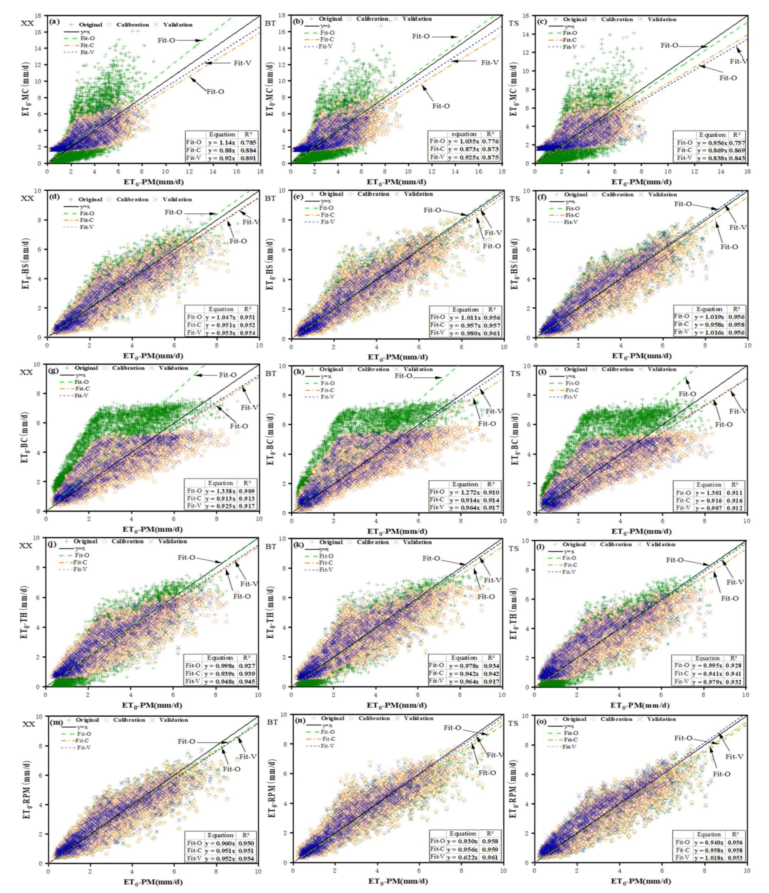
Figure 4 shows scatterplots for ET₀ estimated by the five models and ASCE-PM for the calibration and validation periods for representative WS of BT, TS, and XX. These results show that, before regional calibration, ET_0,MC was significantly greater than ET_0,P and that ET₀ estimated using RPM was closest to ET_0,P. The ET_0,HS and ET_0,TH calculated before calibration were evenly distributed on both sides of y = x, which indicates that the calculated values of these two models were close to ET_0,P. ET_0,BC was generally greater than ET_0,P. ET₀ values calculated by the five calibrated models were closer to the line y = x than the uncalibrated models. Regional calibration increased the goodness-of-fit between all of the ET₀ values calculated by the five models and ET_0,P.

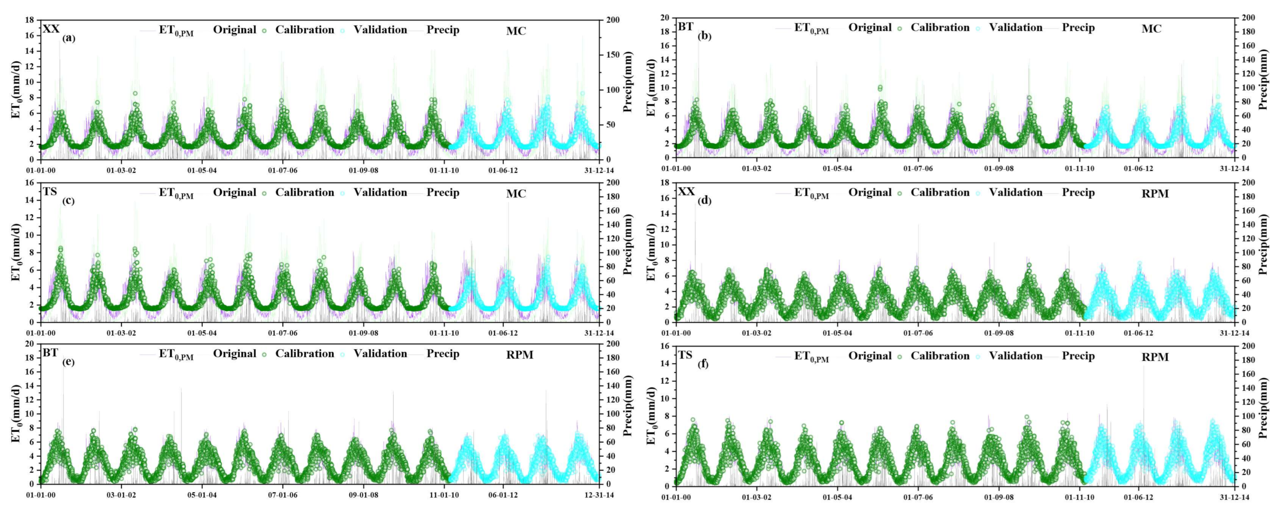
Figure 5 shows the variations in ET₀ estimated by MC, RPM models, and ASCE-PM and Precipitation (Precip) for the three representative stations (for clarity, only the best model RPM and worst model MC are presented). After the calibration, although the maximum value of ET₀ estimated by the five models was slightly less than the ground truth value, the estimated ET₀ agreed well with ET_0,P. That the maximum value of ET_0,MC before calibration was much greater than ET_0,P and that ET_0,MC after calibration fitted ET_{0 P} well. ET_0,RPM fitted well with ET_0,P both before and after calibration. However, the high value of ET₀ estimated by the RPM model in the validation period is still lower than that of ET_0,P, which is the main reason why the estimation accuracy of the RPM model is up to 98%. The estimation accuracy of the HS, TH, and BC models is between MC and RPM models. The low value of ET₀ estimated by the BC model is closer to ET_0,P than ET_0,MC, making the estimation accuracy of the BC model in NCP 84% higher than that of the MC model. The comparison between the daily precipitation of representative stations with ET_0,P shows that ET_0,P is high on rainy days, which indicates that there is a positive correlation between precipitation and ET_0,P. Liu et al. [49] compared the performance of several temperature models for north China and found that the ET₀ calculated by HS well fitted FAO56-PM, which is consistent with our study. Awal et al. [50] evaluated the HS equation with FAO-ET₀ at 88 stations of West Texas Mesonet and concluded that the monthly calibrated HS model yielded a performance (R² = 0.82). Rodrigues and Braga [51] estimated ET₀ during the irrigation season using nine temperature-based methods in a hot-summer Mediterranean climate. The results showed that the modified HS performed acceptably with a R² higher than 0.78. Liu [52] evaluated six temperature-based PET methods, showing that the HS equation was the closeted to the PM calculation values (correlation coefficient = 0.85), followed by the Oudin and Hamon equations, whereas the revised Thornthwaite and Baier–Robertson equations performed relatively poorly. These agreed well with results in the study, and our studies performed better in some cases. Our results indicated that calibration increased the accuracy of all of the models’ ET₀ estimation for the study area. Among them, the estimation accuracy of the modified MC model and the modified BC model is greatly improved, by 18% and 19% respectively, so that the calibrated models are suitable for practical use in the local area. The above results indicated that the five calibrated models can be used for ET₀ forecasting.

3.3. ET₀ Forecasts

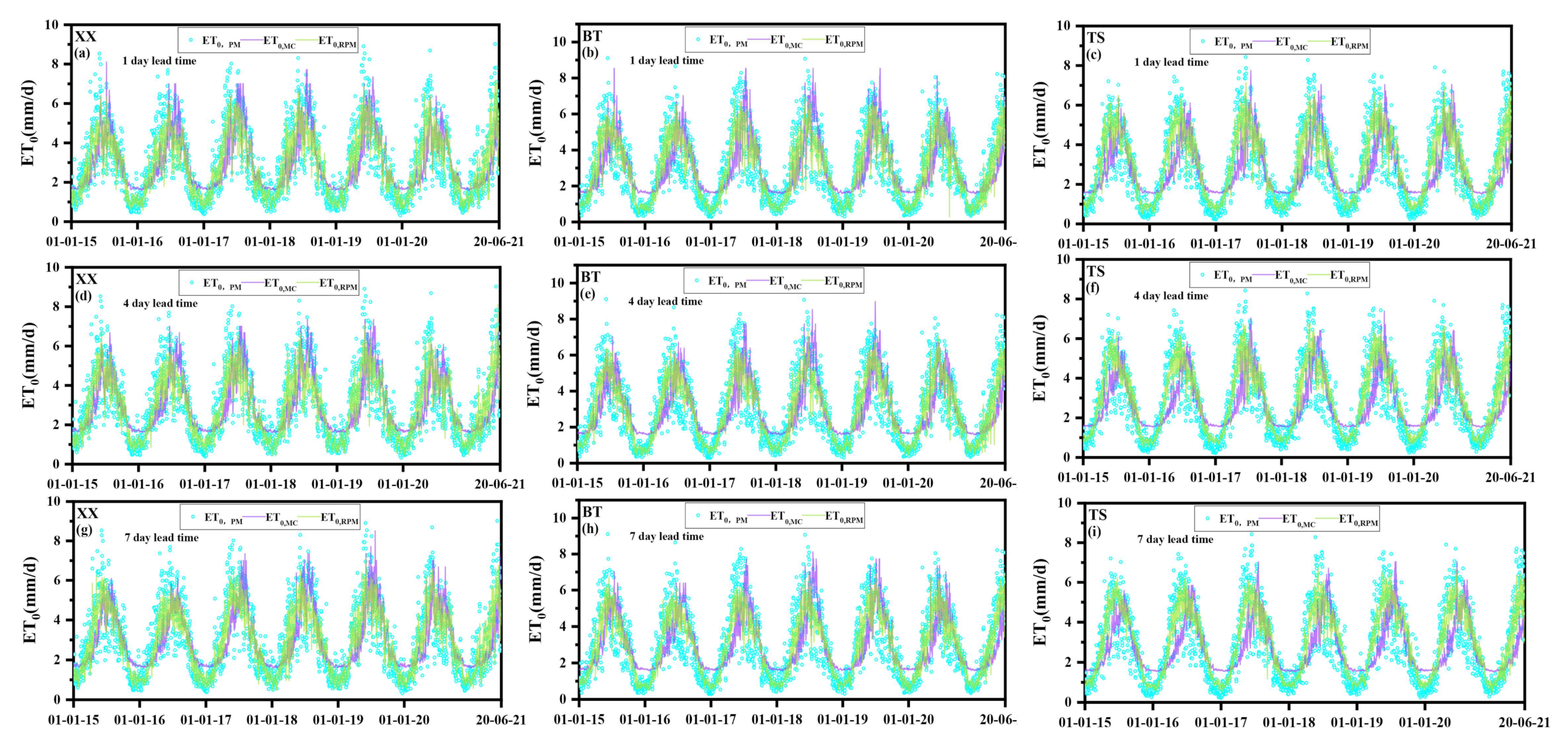
Figure 6 shows a plot of the 1 d ahead, 4 d ahead, and 7 d ahead ET₀ forecasts for three representatives WS in NCP for the period 1 January 2015 to 20 June 2021. These results show that forecast ET₀ has the same trend as the measured ET_0,P for all models. The minimum value of ET_0,MC was greater than the minimum value of ET_0,P, and there was an obvious difference between ET_0,BC and ET_0,P. ET_0,RPM and ET_0,HS were similar, and both were less than ET_0,P. This is consistent with the previous findings that RPM and HS underestimate ET_0,P [33,42]. Forecasts of ET_0,BC were similar to those of ET_0,MC, but the lower values of ET_0,BC were closer to ET_0,P. Predictions of ET_0,TH were less accurate than the values of ET_0,RPM and ET_0,HS but more accurate than forecasts of ET_0,MC and ET_0,BC. The errors show that the forecasts of the five models differ from ET_0,P, and it is evident that the accuracy of the ET₀ forecasting is determined by the computational model used.

Table 5. Average values of the statistical indicators of five temperature-based models’ ET₀ forecast accuracy for 17 stations in 1–7 d ahead forecasts for the NCP.

Statistical Indicator	Lead Time	MC	HS	BC	TH	RPM
Acc (%)	1	75	87	81	84	87
	2	75	86	81	83	86
	3	75	86	81	83	86
	4	75	85	81	82	85
	5	75	85	81	82	85
	6	75	84	81	82	84
	7	75	84	81	81	84
	M	75	85	81	82	85
MAE (mm/d)	1	1.11	0.74	0.87	0.83	0.75
	2	1.11	0.76	0.88	0.85	0.77
	3	1.11	0.76	0.88	0.85	0.76
	4	1.12	0.78	0.88	0.86	0.78
	5	1.12	0.79	0.88	0.87	0.79
	6	1.12	0.80	0.89	0.88	0.80
	7	1.13	0.81	0.89	0.88	0.81
	M	1.12	0.78	0.88	0.86	0.78
RMSE (mm/d)	1	1.42	1.01	1.14	1.10	1.00
	2	1.43	1.03	1.16	1.12	1.03
	3	1.43	1.03	1.15	1.12	1.02
	4	1.43	1.05	1.16	1.13	1.05
	5	1.44	1.06	1.16	1.15	1.06
	6	1.45	1.08	1.16	1.16	1.07
	7	1.45	1.10	1.17	1.17	1.09
	M	1.44	1.05	1.16	1.13	1.05
R	1	0.67	0.86	0.80	0.82	0.86
	2	0.66	0.85	0.80	0.81	0.85
	3	0.66	0.85	0.80	0.81	0.85
	4	0.66	0.84	0.80	0.81	0.84
	5	0.66	0.84	0.79	0.80	0.84
	6	0.65	0.84	0.79	0.80	0.83
	7	0.65	0.83	0.79	0.79	0.83
	M	0.66	0.84	0.80	0.81	0.84

Note: M stands for the mean value of the statistical indicators of 1–7 d ahead ET₀ forecasts by five temperature-based models for 17 stations in the NCP.

presents the average values of the four statistical indicators of ET₀ forecast accuracy for the 17 WS in the 1–7 d ahead forecasting period in NCP. The Acc and R decreased, and the MAE and RMSE increased as the forecast time increased. The Acc for MC for the 7 d ahead forecast was >75%, and R for the same forecast was greater than 0.65. The Acc for the 7 d ahead forecast was greater than 80%, and the R for the same forecast was greater than 0.79 for the other four models. The MAE and RMSE for 7 d ahead forecasts were greater for MC than for the other four models. The greatest average values of MAE (0.1 mm/d) and RMSE (0.2 mm/d) were for MC forecasts. The changes in the four statistical indicators show that the ET₀ forecasts of each model become less accurate as the forecast time increases, which is consistent with the trend of temperature forecasts. However, the ET₀ forecast accuracy of the five models’ maximum decreased by 3% less than the decrease in temperature forecasts.

With the above analysis, the highest average forecast accuracy of the RPM model is 85%, and the lowest average forecast accuracy of the MC model is 75%. The reason for the greater accuracy of RPM may be that the model is conceptually similar to ASCE-PM. In practice, the forecast of ET₀ using RPM is fundamental to irrigation decision-making, a view that has been expressed in other studies [42]. ET_0,HS was second in accuracy, and the originally uncalibrated HS model’s average forecast accuracy was 84%, which indicates that the architecture of the model is suitable for ET₀ forecasts. The forecast accuracy of TH and BC ranked third and fourth. Xiong et al. [5] forecast ET₀ using a monthly calibrated BC equation using temperature forecasts in east China, and the accuracy of the ET₀ forecasting was acceptable (MAE varied between 0.73 and 0.82 mm/d, and R ranged from 0.74 to 0.90). According to the study of Chang et al. [35], a modified daily Thornthwaite (TH) equation can be used to forecast ET₀ with temperature forecasts and found that the RMSE of forecasting ranged from 0.86 to 1.01 mm/d. The results were slightly better than this study, and it may be explained that the performance of the annually calibrated BC and TH model for ET₀ forecast is further improved after monthly calibration. Yang et al. [42] studied representative meteorological stations in different climate zones in China and found that the calibrated TH equation can better forecast the daily ET₀ in different climate zones in China. It agrees well with this study that BC and MC were the fourth and worst choices for daily ET₀ forecasts in the NCP climate zone, compared to RPM, HS, and TH. The reason for the worse performance of BC and MC may be related to the purposes for which the models were created; the BC equation was developed to use U.S. national experimental data, and the MC equation was first used to calculate ET₀ for grass and golf courses in Florida. For a while, the calibrated RPM and HS models were better than the other models, and thus these two models were recommended for short-term ET₀ forecasting in NCP.

Daily ET₀ prediction using the public weather forecast information can be adopted for an irrigation decision support system and real-time water allocation [41,53]. Zhang et al. [54] proposed a methodology to forecast short-term daily ET_c using the ‘Kc-ETo’ approach and public weather forecasts. Considering a basic database for the short-term predicted ET_c of different crops in the whole growth stages and irrigation system engineering information, the irrigation decision support system can make efficient decisions for water allocation with the help of real-time, in-field moisture detection and automatic weather forecast acquisition [55]. It uses technical methods to reduce requirements of a user’s specialized knowledge and can take a user’s managerial experience into account. It can also maximize their productivity and improve irrigation water-use efficiency [56,57].

3.4. Sensitivity and Error Analysis

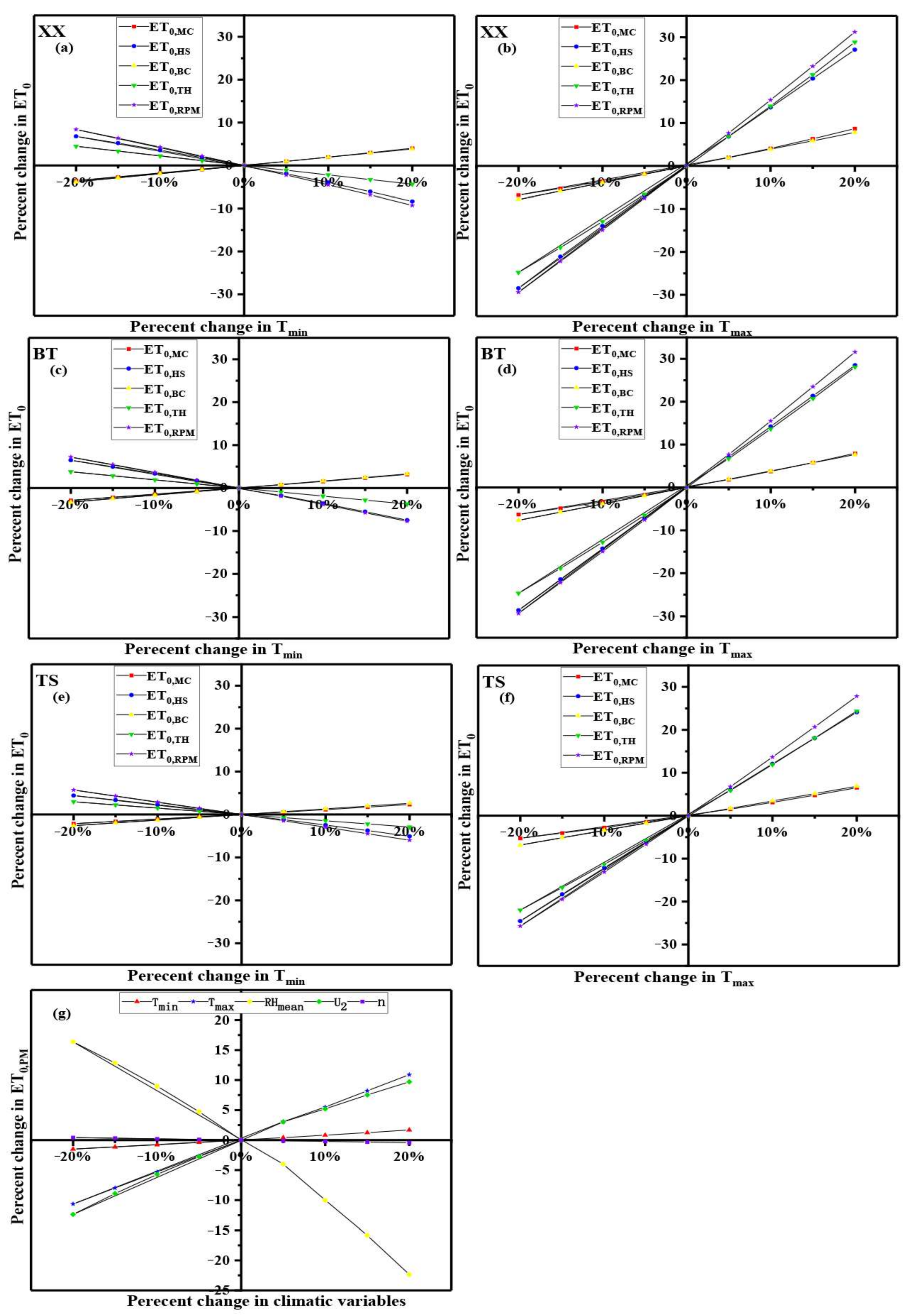
The daily average minimum and maximum air temperatures for representative WS for the past 40 years were used as baseline values, and sensitivity analysis was performed by varying 5 to 20% in 5% from these base values. The amount of increase or decrease in ET₀ with a 5, 10, 15, and 20% increase or decrease in maximum and minimum air temperature was calculated [35]. The percentage changes in ET₀ forecasts for representative WS versus the percentage changes in maximum and minimum air temperatures are shown in Figure 7.

The percentage changes in ET₀ for the five temperature-based models varied linearly with the percentage changes in T_max and T_min but at a greater rate, which indicates that T_max has greater influence on ET₀ forecast than T_min. Other studies have also found that ET₀ is most sensitive to maximum air temperature [35,58]. The preceding analysis of forecast temperature accuracy showed that forecast T_min was more accurate than forecast T_max, so the increased accuracy of the T_max forecast will influence the accuracy of the five models.

The ET_0,MC and EC_0,BC decreased as T_min decreased and increased as T_min increased, and the change trend is consistent with that of T_max. The ET_0,HS, ET_0,Th, and ET_0,RPM behave oppositely, and HS, TS, and RPM were more sensitive to T_min than BC and MC. ET_0,HS, ET_0,TH, and ET_0,RPM changed greatly as T_max changed. Although the change trend was the same as for ET_0,BC and ET_0,MC, the range of the change was greater. Figure 7 shows that the percentage change in ET_0,MC varied from −4% to 5% with the percentage change in T_min and from −7% to 9% with the percentage change in T_max, which was similar to the behavior of ET_0,BC. The percentage change in ET_0,RPM varied from −9% to 8% with the percentage change in T_min and from −29% to 32% with the percentage change in T_max. The percentage change in ET_0,HS varied from −8% to 7% with the percentage change in T_min and from −29% to 29% with the percentage change in T_max. The percentage change in ET_0,TH varied from −4% to 5% with the percentage change in T_min and from −25% to 29% with the percentage change in T_max. This indicates that HS, TH, and RPM are much more sensitive to temperature than BC and MC.

Change in temperature had the greatest influence on RPM, followed in descending order by HS, TH, MC, and BC. This order corresponds almost exactly to the ET₀ forecast accuracy order of the five models for the NCP. Our results are consistent with those of Yang et al. [42], who found that, when the same input data is used, differences in forecast accuracy clearly reflect the quality of the model architecture. Figure 7g shows the influence of variables on the ASCE-PM model, including T_max, T_min, wind speed (U₂), mean relative humidity (RH_mean), and sunshine hours (n). These results show T_max has a greater impact on ET_0,PM than T_min. According to the study of G. T. Patle and D. K. Singh [58], the more sensitive the model is to the maximum temperature, the better the ET₀ forecast performance would be. The ET₀ forecast error factors might be divided into two categories. The errors in temperature forecasts directly influenced the ET₀ forecast accuracy, and the effects of wind and relative humidity are not taken into account when forecasting ET₀ [51]. With an increase in the temperature forecast accuracy, especially in maximum temperature, the model performance can be improved.

4. Conclusions

We used five temperature-based models, MC, HS, BC, TH, and RPM, to make daily forecasts of ET₀ for a 1 to 7 d ahead period for 1 January 2015 to 20 June 2021 using public weather forecasts from 17 WS in the NCP. We investigated the accuracy of temperature forecasts and analyzed the sensitivity of each model to air temperature. The main conclusions are as follows.

Forecasts of T_min were more accurate than forecasts of T_max, and forecast temperature accuracy decreased by 14% as the forecast period increased. The accuracy of ET₀ forecasts by the five models similarly decreased by 3% as the period of the forecast increased. The forecast accuracy of the five calibrated models was all greater than 75%. All five calibrated temperature-based models can be used for short-term ET₀ forecasts for NCP, but RPM, HS, and TH are, in that order, more accurate than BC or MC. Therefore, the calibrated RPM and HS models were better than the other models and thus these two equations were recommended for short-term ET₀ forecasting in NCP.

Sensitivity analysis showed that T_max had greater influence on the ET₀ forecast than T_min. Changes in temperature had the greatest influence on RPM, followed in descending order by HS, TH, MC, and BC. The ET₀ forecast error factors might be in two categories. The errors in temperature forecasts directly influenced the ET₀ forecast accuracy, while other weather factors not considered in the temperature-based model also caused ET₀ forecast errors. With an increase in the temperature forecast accuracy, especially in maximum temperature, the model performance can be improved.

The five calibrated models described herein can be used to forecast crop water and irrigation water requirements over a 7-day forecast horizon. Public weather forecast data at the provincial level can now be directly used for ET₀ forecasts to be used as an irrigation scheduling decision support tool for direct field applications in crop cultivation in the NCP. Although we have taken the results provided by the ASCE-PM equation as the benchmark values, it should be noted that this is also a calculation model, which may be inadequate for some cases. It would be therefore much more reliable to attempt to improve five equations based on actual lysimeter measurements.

References

1. He, C.; Wang, Y.Q.; Yu, W.B.; Kou, Y.H.; Yves, B.N.d.; Zhao, X.; Zhang, H.L. Comprehensive Analysis of Resource Utilization Efficiency under Different Tillage Systems in North China Plain. J. Clean. Prod. 2022, 347, 131289. [Google Scholar] [CrossRef]
2. Yang, G.; Li, S.; Wang, H.; Wang, L. Study on Agricultural Cultivation Development Layout Based on the Matching Characteristic of Water and Land Resources in North China Plain. Agric. Water Manag. 2022, 259, 107272. [Google Scholar] [CrossRef]
3. Koch, J.; Zhang, W.; Martinsen, G.; He, X.; Stisen, S. Estimating Net Irrigation Across the North China Plain Through Dual Modeling of Evapotranspiration. Water Resour. Res. 2020, 56, e2020WR027413. [Google Scholar] [CrossRef]
4. Zhang, Z.; Lin, A.; Zhao, L.; Zhao, B. Attribution of Local Land Surface Temperature Variations Response to Irrigation over the North China Plain. Sci. Total Environ. 2022, 826, 154104. [Google Scholar] [CrossRef] [PubMed]
5. Xiong, Y.; Luo, Y.; Wang, Y.; Traore, S.; Xu, J.; Jiao, X.; Fipps, G. Forecasting Daily Reference Evapotranspiration Using the Blaney-Criddle Model and Temperature Forecasts. Arch. Agron. Soil Sci. 2015, 62, 790–805. [Google Scholar] [CrossRef]
6. Srivastava, A.; Sahoo, B.; Raghuwanshi, N.S.; Singh, R. Evaluation of Variable-Infiltration Capacity Model and MODIS-Terra Satellite-Derived Grid-Scale Evapotranspiration Estimates in a River Basin with Tropical Monsoon-Type Climatology. J. Irrig. Drain. Eng. 2017, 143, 1. [Google Scholar] [CrossRef]
7. Allen, R.G.; Walter, I.A.; Elliot, R.L.; Howell, T.A.; Su, D.I.; Jensen, M.E.; Snyder, R.L. The ASCE Standardized Reference Evapotranspiration Equation; American Society of Civil Engineers: Reston, VA, USA, 2005. [Google Scholar] [CrossRef]
8. Monteith, J.L. Evaporation and Environment. In Symposia of the Society for Experimental Biology; Cambridge University Press: Cambridge, UK, 1965; Volume 19, pp. 205–234. [Google Scholar]
9. Doorenbos, J.; Pruitt, W.O. Guidelines for Prediction of Crop Water Requirements; FAO Irrigation and Drainage Paper No. 24; FAO: Rome, Italy, 1977. [Google Scholar]
10. Wright, J.L. Derivation of alfalfa and grass reference evapotranspiration. In Evapotranspiration and Irrigation Scheduling; ASAE: San Antonio, TX, USA, 1996; pp. 133–140. [Google Scholar]
11. Wright, J.L.; Jensen, M.E. Peak Water Requirements of Crops in Southern Idaho. J. Irrig. Drain. Div. 1972, 96, 193–201. [Google Scholar] [CrossRef]
12. Wright, J.L. New Evapotranspiration Crop Coefficients. J. Irrig. Drain. Div. 1982, 108, 57–74. [Google Scholar] [CrossRef]
13. Allen, R.G.; Pereira, L.S.; Raes, D.; Smith, M. Crop Evapotranspiration-Guidelines for Computing Crop Water Requirements; FAO Irrigation and drainage paper 56; FAO: Rome, Italy, 1998; Volume 300, p. D05109. [Google Scholar]
14. Allen, R.G.; Smith, M.; Pereira, L.S.; Perrier, A. An Update for the Calculation of Reference Evapotranspiration. ICID Bull. 1994, 43, 35–92. [Google Scholar]
15. Feng, Y.; Peng, Y.; Cui, N.; Gong, D.; Zhang, K. Modeling Reference Evapotranspiration Using Extreme Learning Machine and Generalized Regression Neural Network Only with Temperature Data. Comput. Electron. Agric. 2017, 136, 71–78. [Google Scholar] [CrossRef]
16. Landeras, G.; Ortiz-Barredo, A.; López, J.J. Forecasting Weekly Evapotranspiration with ARIMA and Artificial Neural Network Models. J. Irrig. Drain. Eng. 2009, 135, 323–334. [Google Scholar] [CrossRef]
17. Yassin, M.A.; Alazba, A.A.; Mattar, M.A. Artificial Neural Networks versus Gene Expression Programming for Estimating Reference Evapotranspiration in Arid Climate. Agric. Water Manag. 2016, 163, 110–124. [Google Scholar] [CrossRef]
18. Ladlani, I.; Houichi, L.; Djemili, L.; Heddam, S.; Belouz, K. Estimation of Daily Reference Evapotranspiration (ET0) in the North of Algeria Using Adaptive Neuro-Fuzzy Inference System (ANFIS) and Multiple Linear Regression (MLR) Models: A Comparative Study. Arab. J. Sci. Eng. 2014, 39, 5959–5969. [Google Scholar] [CrossRef]
19. Traore, S.; Luo, Y.; Fipps, G. Deployment of Artificial Neural Network for Short-Term Forecasting of Evapotranspiration Using Public Weather Forecast Restricted Messages. Agric. Water Manag. 2015, 163, 363–379. [Google Scholar] [CrossRef]
20. Abdullah, S.S.; Malek, M.A.; Abdullah, N.S.; Kisi, O.; Yap, K.S. Extreme Learning Machines: A New Approach for Prediction of Reference Evapotranspiration. J. Hydrol. 2015, 527, 184–195. [Google Scholar] [CrossRef]
21. Gocic, M.; Petković, D.; Shamshirband, S.; Kamsin, A. Comparative Analysis of Reference Evapotranspiration Equations Modelling by Extreme Learning Machine. Comput. Electron. Agric. 2016, 127, 56–63. [Google Scholar] [CrossRef]
22. Fan, J.; Yue, W.; Wu, L.; Zhang, F.; Cai, H.; Wang, X.; Lu, X.; Xiang, Y. Evaluation of SVM, ELM and Four Tree-Based Ensemble Models for Predicting Daily Reference Evapotranspiration Using Limited Meteorological Data in Different Climates of China. Agric. For. Meteorol. 263 2018, 225–241. [Google Scholar] [CrossRef]
23. Ferreira, L.B.; da Cunha, F.F.; de Oliveira, R.A.; Fernandes Filho, E.I. Estimation of Reference Evapotranspiration in Brazil with Limited Meteorological Data Using ANN and SVM—A New Approach. J. Hydrol. 2019, 572, 556–570. [Google Scholar] [CrossRef]
24. Granata, F. Evapotranspiration Evaluation Models Based on Machine Learning Algorithms—A Comparative Study. Agric. Water Manag. 2019, 217, 303–315. [Google Scholar] [CrossRef]
25. Droogers, P.; Allen, R.G. Estimating Reference Evapotranspiration under Inaccurate Data Conditions. Irrig. Drain. Syst. 2002, 16, 33–45. [Google Scholar] [CrossRef]
26. Hargreaves, G.H.; Samani, Z.A. Reference Crop Evapotranspiration From Ambient Air Temperature. Pap.-Am. Soc. Agric. Eng. 1985, 1, 96–99. [Google Scholar]
27. Thornthwaite, C.W. An Approach toward a Rational Classification of Climate. Geogr. Rev. 1948, 38, 55–94. [Google Scholar] [CrossRef]
28. Blaney, H.F.; Criddle, W.D. Determining Consumptive Use and Irrigation Water Requirements; US Department of Agriculture: Washington, DC, USA, 1962.
29. Trajkovic, S. Temperature-Based Approaches for Estimating Reference Evapotranspiration. J. Irrig. Drain. Eng. 2005, 131, 316–323. [Google Scholar] [CrossRef]
30. Lu, J.; Sun, G.; Mcnulty, S.; Amatya, D.M. A Comparison of Six Potential Evapotranspiration Methods for Regional Use in the Southeastern United States. J. Am. Water Resour. Assoc. 2005, 41, 621–633. [Google Scholar] [CrossRef]
31. Zhang, Q.; Duan, A.; Wang, G.; Shiva, J.K.; Shen, X.; Cai, H. Middle and Short Term Forecasting Models for Reference Evapotranspiration Based on Daily Weather Forecast. Nongye Jixie Xuebao/Trans. Chin. Soc. Agric. Mach. 2015, 46, 107–114. [Google Scholar] [CrossRef]
32. Ren, X.; Qu, Z.; Martins, D.S.; Paredes, P.; Pereira, L.S. Daily Reference Evapotranspiration for Hyper-Arid to Moist Sub-Humid Climates in Inner Mongolia, China: I. Assessing Temperature Methods and Spatial Variability. Water Resour. Manag. 2016, 30, 3769–3791. [Google Scholar] [CrossRef]
33. Feng, Y.; Jia, Y.; Cui, N.; Zhao, L.; Li, C.; Gong, D. Calibration of Hargreaves Model for Reference Evapotranspiration Estimation in Sichuan Basin of Southwest China. Agric. Water Manag. 2017, 181, 1–9. [Google Scholar] [CrossRef]
34. Zhu, X.; Luo, T.; Luo, Y.; Yang, Y.; Guo, L.; Luo, H.; Fang, C.; Cui, Y. Calibration and Validation of the Hargreaves-Samani Model for Reference Evapotranspiration Estimation in China. Irrig. Drain. 2019, 68, 822–836. [Google Scholar] [CrossRef]
35. Chang, X.; Wang, S.; Gao, Z.; Luo, Y.; Chen, H. Forecast of Daily Reference Evapotranspiration Using a Modified Daily Thornthwaite Equation and Temperature Forecasts. Irrig. Drain. 2018, 68, 297–317. [Google Scholar] [CrossRef]
36. Chen, D.; Gao, G.; Xu, C.Y.; Guo, J.; Ren, G. Comparison of the Thornthwaite Method and Pan Data with the Standard Penman-Monteith Estimates of Reference Evapotranspiration in China. Clim. Res. 2005, 28, 123–132. [Google Scholar] [CrossRef]
37. Rahimikhoob, A.; Hosseinzadeh, M. Assessment of Blaney-Criddle Equation for Calculating Reference Evapotranspiration with NOAA/AVHRR Data. Water Resour. Manag. 2014, 28, 3365–3375. [Google Scholar] [CrossRef]
38. Luo, Y.; Li, S.; Peng, S.; Wang, W.; Jiao, X.; Jiang, Y.; Gu, H. Forecasting Reference Crop Evapotranspiration Based on Temperature Forecast and Hargreaves—Samani Equation. J. Drain. Irrig. Mach. Eng. 2013, 31, 987–992. [Google Scholar]
39. Wang, W.; Xing, W.; Shao, Q. How Large Are Uncertainties in Future Projection of Reference Evapotranspiration through Different Approaches? J. Hydrol. 2015, 524, 696–700. [Google Scholar] [CrossRef]
40. Liu, B.; Liu, M.; Cui, Y.; Shao, D.; Mao, Z.; Zhang, L.; Khan, S.; Luo, Y. Assessing Forecasting Performance of Daily Reference Evapotranspiration Using Public Weather Forecast and Numerical Weather Prediction. J. Hydrol. 2020, 590, 125547. [Google Scholar] [CrossRef]
41. Luo, Y.; Chang, X.; Peng, S.; Khan, S.; Wang, W.; Zheng, Q.; Cai, X. Short-Term Forecasting of Daily Reference Evapotranspiration Using the Hargreaves-Samani Model and Temperature Forecasts. Agric. Water Manag. 2014, 136, 42–51. [Google Scholar] [CrossRef]
42. Yang, Y.; Luo, Y.; Wu, C.; Zheng, H.; Zhang, L.; Cui, Y.; Sun, N.; Wang, L. Evaluation of Six Equations for Daily Reference Evapotranspiration Estimating Using Public Weather Forecast Message for Different Climate Regions across China. Agric. Water Manag. 2019, 222, 386–399. [Google Scholar] [CrossRef]
43. Mohawesh, O.E. Spatio-Temporal Calibration of Blaney-Criddle Equation in Arid and Semiarid Environment. Water Resour. Manag. 2010, 24, 2187–2201. [Google Scholar] [CrossRef]
44. McCloud, D.E. Water requirements of field crops in Florida as influenced by climate. Proc. Soil Sci. Soc. Fla. 1995, 15, 165–172. [Google Scholar]
45. Pereira, A.R.; Pruitt, W.O. Adaptation of the Thornthwaite Scheme for Estimating Daily Reference Evapotranspiration. Agric. Water Manag. 2004, 66, 251–257. [Google Scholar] [CrossRef]
46. Yang, Y.; Cui, Y.; Bai, K.; Luo, T.; Dai, J.; Wang, W.; Luo, Y. Short-Term Forecasting of Daily Reference Evapotranspiration Using the Reduced-Set Penman-Monteith Model and Public Weather Forecasts. Agric. Water Manag. 2019, 211, 70–80. [Google Scholar] [CrossRef]
47. China Meteorological Administration (CMA). Quality Inspection of Medium-Short-Term Weather Forecast; Meteorology Press: Beijing, China, 2005. (In Chinese) [Google Scholar]
48. Irmak, S.; Allen, R.G.; Whitty, E.B. Daily Grass and Alfalfa-Reference Evapotranspiration Estimates and Alfalfa-to-Grass Evapotranspiration Ratios in Florida. J. Irrig. Drain. Eng. 2003, 129, 360–370. [Google Scholar] [CrossRef]
49. Liu, X.; Li, Y.; Wang, Q. Evaluation on Several Temprature-Based Methods for Estimating Reference Crop Evapotranspiration. Trans. CSAE 2006, 22, 12. [Google Scholar]
50. Awal, R.; Habibi, H.; Fares, A.; Deb, S. Estimating Reference Crop Evapotranspiration under Limited Climate Data in West Texas. J. Hydrol. Reg. Stud. 2020, 28, 100677. [Google Scholar] [CrossRef]
51. Rodrigues, G.C.; Braga, R.P. Estimation of Reference Evapotranspiration during the Irrigation Season Using Nine Temperature-Based Methods in a Hot-Summer Mediterranean Climate. Agriculture 2021, 11, 124. [Google Scholar] [CrossRef]
52. Liu, Z. Estimating Land Evapotranspiration from Potential Evapotranspiration Constrained by Soil Water at Daily Scale. Sci. Total Environ. 2022, 834, 155327. [Google Scholar] [CrossRef]
53. Cai, J.B.; Liu, Y.; Xu, D.; Paredes, P.; Pereira, L.S. Simulation of the Soil Water Balance of Wheat Using Daily Weather Forecast Messages to Estimate the Reference Evapotranspiration. Hydrol. Earth Syst. Sci. 2009, 13, 1045–1059. [Google Scholar] [CrossRef]
54. Zhang, L.; Cui, Y.; Xiang, Z.; Zheng, S.; Traore, S.; Luo, Y. Short-Term Forecasting of Daily Crop Evapotranspiration Using the ‘Kc-ETo’ Approach and Public Weather Forecasts. Arch. Agron. Soil Sci. 2018, 64, 903–915. [Google Scholar] [CrossRef]
55. Wang, W.; Cui, Y.; Luo, Y.; Li, Z.; Tan, J. Web-Based Decision Support System for Canal Irrigation Management. Comput. Electron. Agric. 2019, 161, 312–321. [Google Scholar] [CrossRef]
56. Kim, Y.; Evans, R.G. Software Design for Wireless Sensor-Based Site-Specific Irrigation. Comput. Electron. Agric. 2009, 66, 159–165. [Google Scholar] [CrossRef]
57. Chauhan, Y.S.; Wright, G.C.; Holzworth, D.; Rachaputi, R.C.N.; Payero, J.O. AQUAMAN: A Web-Based Decision Support System for Irrigation Scheduling in Peanuts. Irrig. Sci. 2013, 31, 271–283. [Google Scholar] [CrossRef]
58. Patle, G.T.; Singh, D.K. Sensitivity of Annual and Seasonal Reference Crop Evapotranspiration to Principal Climatic Variables. J. Earth Syst. Sci. 2015, 124, 819–828. [Google Scholar] [CrossRef] [Green Version]
Figure 1. Location of the 17 weather stations used in this study. The red sites Xinxiang (XX), Botou (BT), and Tangshan (TS) are representative of the north–south and east–west geographic locations.
Water 14 02888 g001
Figure 2. Workflow of the ET0 forecasting in this study.
Water 14 02888 g002
Figure 3. Statistical indices for daily minimum temperature forecasts: (a) Accuracy, (b) MAE, (c) RMSE, and (d) R; for daily maximum temperature forecasts: (e) Accuracy, (f) MAE, (g) RMSE, and (h) R at 17 stations.
Water 14 02888 g003
Figure 4. Scatterplots for ET0 calculated by the temperature-based models and the PM model for original, calibrated, and validated models in stations BT, TS, and XX; (ac) MC model, (df) HS model, (gi) BC model, (jl) TH model, (mo) RPM model; Fit-O, Fit-C, and Fit-V are respectively the best fit lines for the original, calibrated, and validated models.
Water 14 02888 g004
Figure 5. Variation in ET0 estimated by the MC and RPM temperature-based models and PM and Precipitation (Precip) for stations BT, TS, and XX; (ac) MC model and the (df) RPM model.
Water 14 02888 g005
Figure 6. Comparisons of ET0 forecasts between MC and RPM temperature-based models and PM for BT, TS, and XX; (ac) 1 d ahead, (df) 4 d ahead, and (gi) 7 d ahead.
Water 14 02888 g006
Figure 7. Percentage change in ET0 forecasts with respect to the percentage change in temperature for stations BT, TS, and XX; Tmin (a,c,e), Tmax (b,d,f); percentage change in ET0,PM with respect to the percentage change in climatic variables (g).
Water 14 02888 g007