Article

Flood-Frequency Analysis for Dams in Romania

by
Cornel Ilinca
* and
Cristian Gabriel Anghel
Faculty of Hydrotechnics, Technical University of Civil Engineering Bucharest, Lacul Tei, nr.122-124, 020396 Bucharest, Romania
*
Author to whom correspondence should be addressed.
Water 2022, 14(18), 2884; https://doi.org/10.3390/w14182884
Submission received: 16 August 2022 / Revised: 5 September 2022 / Accepted: 10 September 2022 / Published: 15 September 2022
(This article belongs to the Section Hydrology)

Abstract

:
Accurately determining the maximum designed water discharges of dams is extremely important, considering the economic costs of carrying out these types of hydrotechnical works and the possible disastrous consequences resulting from their incorrect design. This article describes and applies probability distributions used in hydrology, with some recommended by Romanian legislation standard NP 129-2011. The methods for estimating the parameters presented in this article, as well as the establishment of directions for correlating the normative with international regulations, resulting from the research on many rivers with different characteristics, conducted within the Faculty of Hydrotechnics, were completed with specialized computer applications for applying the normative. In this article, two case studies reflecting this research are presented. The verification of the proposed recommendations, on rivers with hydrographic basins with different physiographic characteristics, confirmed the opportunity to implement rigorous and simple criteria. The presentation of the quantile form of some distributions (especially Pearson III) and of the expressions of moments (central and raw) of high order, as well as the presentation of the frequency factors of each analyzed distribution necessary to calculate the confidence interval, constitute novelties, thus facilitating the ease of use of these distributions.

1. Introduction

According to the Romanian legislation, the water dams are designed and verified at the values of the maximum water discharges with different probabilities of being exceeded [1], depending on the importance class of the dams [2].
Rigorous determination of these maximum flows is of particular importance given the costs and risks associated with these types of hydrotechnical works, especially in the context of climate change. The availability of hydrological data from the last period allows the recalculation of maximum flows for the imposition of constructive/non-constructive measures regarding the increase of the capacity of large water discharges.
For a better prediction of floods and the adoption of appropriate mitigation and protection measures, it is essential to know the hydrological and hydraulic characteristics of watercourses [3].
The current legislation [4] requires a correlation with international recommendations and modern practices, as well as the implementation of computer applications for the normative, to be used by engineers without advanced knowledge of mathematics and computer science.
In Romania, the method of ordinary moments (MOM) is established, but taking into account the fact that hydrometric monitoring is deficient, in most cases, the data series are not older than 25 years, and it is necessary to achieve a regionalization based on the L-moments method [5,6], which is generally a method less influenced by the length of the data series and the existence of extreme values. Another solution is the use of partial series (POT), which is much more laborious to achieve, requiring additional checks of data independence and criteria for establishing threshold values [7,8,9].
The comparative presentation, in this article, of the two methods for estimating the parameters, MOM and L-moments, for certain distributions used in Romania and correlated with international regulations [10,11,12] represents a starting point in achieving a regionalization based on the L-moments method. It should be emphasized that the L-moments method has not been presented, analyzed and applied to specific hydrography in Romania. Switching to the L-moment can be done by linear regressions between the coefficient of variation based on the MOM (CV) and the coefficient of variation based on L-moments (L-CV), HCS and L-CS, where HCS is Hazen’s unbiased skewness or Cs adopted depending on the genesis of the flows, and L-CS is the L-moment’s skewness. The genesis of the flows represents the generating mechanism of the maximum flows given by the spatio-temporal conditions of the precipitations and the physiographic characteristics of the hydrographic basin [13,14,15].
This article analyses Pearson III, the most used three parameters of statistical distribution in Romania (parent distribution), as well as LogPearson and GEV distributions, which are recommended by the Romanian legislation [4]. In addition to these distributions, two distributions commonly used internationally are analyzed and applied, the LogNormal and the Wakeby distributions [5,10,11,12,16,17,18,19]. This article describes the latest methods for estimating distribution parameters using engineering mathematics software, by presenting, for the first time, some expressions of the functions, moments and frequency factors, facilitating the ease of use of these distributions.
Thus, novelty elements, such as the Pearson III expressions of the probability density function using the dgamma built-in function, the cumulative probability function using pgamma and pchisq built-in functions, the quantile function expressed with qgamma and qchisq functions and the form of the L-skewness coefficient expressed with ibeta and pbeta built-in functions; the LogPearson III expressions of the probability density function using the dgamma function, the cumulative probability function using the pgamma function, the quantile function expressed with the qgamma function, the form of the three L-moments and the expression of the frequency factor; the GEV expression for the third L-moment; the LogNormal expressions of the probability density function using the dnorm built-in function and dlnorm function, the cumulative probability function (using pnorm, plnorm and cnorm functions) and the expressions of the three conditions for L-moments using the quantile function and the Wakeby expressions for high order moments and the frequency factor.
All of these novelty elements help hydrology researchers understand and apply the processes behind dedicated softwares, in which they select some options without knowing the mathematics behind them. We consider that the use of these kinds of softwares (not knowing the mathematics behind them) is not beneficial in the long run.

2. Flood Frequency Analysis—Determination of Maximum Flows

In Romania, the series of maximum flows used to estimate the parameters of statistical distributions are those of the annual maximum series (AM). A disadvantage of this series is that the values resulting from the theoretical distributions are conservative and, in some cases, exaggerated, especially in the field of low probabilities, and there are underestimated values for exceeding probabilities higher than 80%. The probability of exceeding 80% has a special importance because, according to Romanian legislation Order no. 326/2007, it represents a criterion for determining the bankfull channel. Currently, according to Romanian legislation Order no. 2.115/2021, the annual probability of exceeding 50% is used, but it is too high for mountain river areas.
The annual maximum series consists of the values of the maximum flows characterizing each hydrological year. The advantage of this analysis is the certainty of data independence. Large datasets with length n ≥ 20 [12,13,14,15] are required for these analyses. Based on these considerations, it is necessary to impose an analysis based on the L-moments method.
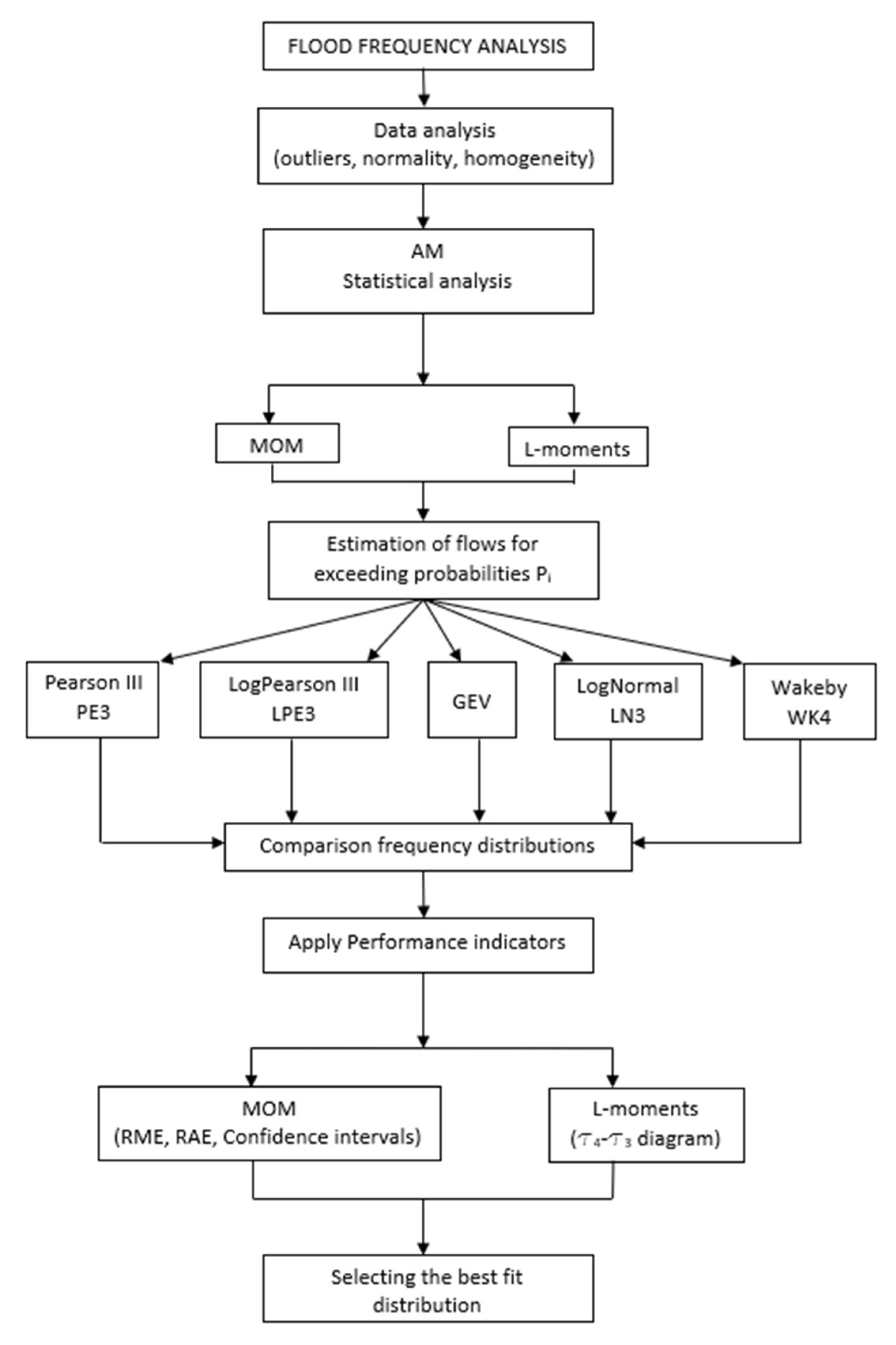
The determination of the maximum flows was carried out in stages, according to Figure 1. The verification of the character of outliers, normality and homogeneity were carried out in the data-curation phase.
In the next section, the theoretical distributions used in this article for the calculation of the maximum flows are presented [5,16,17,19]. Only the notation of MOM and L-moments will be used to represent the two methods of estimating the parameters of statistical distributions.

2.1. Pearson III Distribution (PE3)

Pearson III distribution is a particular case of the four-parameter exponential gamma distribution (FPEGD) under the condition of b = 1. The probability density function of FPEGD is [20]:
f x = β α x γ α b 1 β Γ α exp x γ β 1 b
The probability density function, f x ; the complementary cumulative distribution function, F x , and quantile function, x p , of the Pearson III distribution are:
f x = x γ α 1 β α Γ α exp x γ β = 1 β d g a m m a x γ β , α
F x = 1 1 β Γ α γ x x γ β α 1 exp x γ β d x = Γ α , x γ β Γ α
F x = 1 p g a m m a x γ β , α = 1 p c h i s q 2 x γ β , 2 α
x p = γ + β q g a m m a 1 p , α = μ + σ q g a m m a 1 p , α α α = γ + β q c h i s q 1 p , 2 α = μ + σ q c h i s q 1 p , 2 α 2 α α
where α , β , γ are the shape, the scale and the position parameters, with conditions γ < x < if β > 0 or < x < γ if β < 0 and α > 0 ; μ , σ represent the mean and standard deviation.
Appendix C presents the built-in mathematical functions in Mathcad.

2.2. LogPearson Distribution (LP3)

The probability density function, f x ; the complementary cumulative distribution function, F x , and the quantile function, x p , of the LogPearson distribution are:
f x = ln x γ α 1 x β α Γ α exp ln x γ β = 1 β x d g a m m a ln x γ β , α
F x = Γ α , ln x γ β Γ α = 1 p g a m m a ln x γ β , α
x p = exp γ + β q g a m m a 1 p , α
where α , β , γ are the shape, the scale and the position parameters. For case β > 0 , the quantile takes the form of x p = exp γ + β q g a m m a p , α .

2.3. Generalized Extreme Value Distribution (GEV)

The probability density function, f x ; the complementary cumulative distribution function, F x , and the quantile function, x p , of the GEV distribution are [17]:
f x = 1 α β x γ 1 α 1 1 β exp 1 α β x γ 1 α
F x = 1 exp 1 α β x γ 1 α
x p = γ + β α 1 ln 1 p
where α , β , γ are the shape, the scale and the position parameters; x < γ + β α if α > 0 , and x > γ + β α if α < 0 .

2.4. LogNormal Distribution (LN3)

The probability density function, f x ; the complementary cumulative distribution function, F x , and the quantile function, x p , of the LN3 distribution are:
f x = exp ln x γ α 2 2 β 2 x γ β 2 π = 1 x γ d n o r m ln x γ , α , β = d l n o r m x γ , α , β
F x = 1 1 2 e r f 1 2 β ln x γ α + 1 = 1 p n o r m ln x γ , α , β = 1 c n o r m ln x γ α β = 1 p l n o r m x γ , α , β
x p = γ + exp α + β q n o r m 1 p , 0 , 1 = γ + q l n o r m 1 p , α , β
where α , β , γ are the shape, the scale and the position parameters; μ , σ represent the mean and standard deviation. There are also other forms of expression of the functions [16,17,19].

2.5. Four-Parameters Wakeby Distribution (WK4)

The four-parameters Wakeby distribution represents an alternative to the LogNormal distribution. The four-parameters Wakeby distribution has no form for density and cumulative function, being classified as a quantile function.
The quantile function of WK4 distributions is [5,17]:
x p = α β 1 p β γ δ 1 p δ
where α , γ are the scale parameters, and β , δ are the shape parameters.

3. Method of Parameters Estimation

In this article, two methods of parameters estimation are studied: the MOM and L-moments methods.

3.1. Method of Ordinary Moments (MOM)

In the MOM, the function parameters are obtained from the formulas expressed for the expected value, variance and skewness. In the case of the four parameters Wakeby distribution, it is necessary to express kurtosis as an additional condition.
The formulas for these indicators can be obtained according to the central moments or depending on the raw moments, as follows [17,21,22]:
expected   value :   μ = m 1 = m 1
variance :   σ 2 = m 2 = m 2 m 1 2
skewness :   γ 1 = m 3 m 2 3 / 2 = m 3 3 m 2 m 1 + 2 m 1 3 m 2 m 1 2 3 / 2
kurtosis :   γ 2 = m 4 m 2 2 = m 4 4 m 3 m 1 + 6 m 2 m 1 2 3 m 1 4 m 2 m 1 2 2
E x r = m r = x r f x d x , which represents the raw moment of the r order, and γ 1 = ξ C v , in which ξ is chosen depending on the origin of the flows, namely, 2 if the flows come exclusively from the melting of snow, 3 if the flows have a mixed origin of melting snow and rain and 4 if the flows come exclusively from rain [13,14,15].

3.1.1. Pearson III Distribution

The formulas for expected value, variance and skewness are as follows [10,16,17]:
expected   value :   μ = γ + α β
variance :   σ 2 = α β 2
skewness :   γ 1 = 2 α

3.1.2. LogPearson Distribution (LP3)

The formulas for expected value, variance and skewness are [16]:
expected   value :   μ = exp γ 1 β α
variance :   σ 2 = exp 2 γ 1 1 2 β α 1 1 β 2 α
skewness :   γ 1 = 1 1 3 β α 3 1 2 β α 1 β α + 2 1 β 3 α 1 1 2 β α 1 1 β 2 α 3 2

3.1.3. Generalized Extreme Value Distribution (GEV)

The formulas for expected value, variance and skewness have the following expressions [6,17]:
expected   value :   μ = γ + β α 1 Γ α + 1
variance :   σ 2 = β 2 α 2 Γ 2 α + 1 Γ α + 1 2
skewness:
γ 1 = s i g n α 3 Γ 2 α + 1 Γ α + 1 Γ 3 α + 1 2 Γ α + 1 3 Γ 2 α + 1 Γ α + 1 2 3

3.1.4. LogNormal Distribution (LN3)

The formulas for expected value, variance and skewness are [6,16,17]:
expected   value :   μ = γ + exp α + 1 2 β 2
variance :   σ 2 = exp β 2 + 2 α exp β 2 1
skewness : γ 1 = 3 exp β 2 1 + exp β 2 1 3

3.1.5. Wakeby Distribution (WK4)

Due to complicated expressions, only the formulas for expected value and variance are presented in this section [17].
The expression for skewness is presented in Appendix B.
The expression for kurtosis is obtained based on the raw moments presented in Appendix B.
The WK4 equations are:
expected   value :   μ = α β + 1 γ δ 1
variance:
σ 2 = 2 α 2 β + 1 2 β + 1 α β + 1 γ δ 1 2 2 γ 2 α δ 2 β + 1 γ + 2 α β + 5 α δ + β 2 + 2 β + 1 γ + α β + 2 α β + 1 δ β + 1 δ 1 2 δ 1

3.2. Method of L-Moments

Method of L-Moments is based on linear combinations of probability-weighted moments [5,17]. The flow data must be in ascending order. The formulas for sample L-moments are defined in Appendix A.

3.2.1. Pearson III Distribution

The equations necessary to obtain the exact solution for the parameters of the PE3 function are the following:
L 1 = γ + α β
L 2 = β Γ α + 1 2 π Γ α
τ 3 = 3 2 i b e t a 1 3 , α , 2 α 1   or   τ 3 = 3 2 p b e t a 1 3 , α , 2 α 1
where i b e t a a , x , y and p b e t a x , s 1 , s 2 are explained in Apendix C.
An approximate solution of the parameters depending on the parameter α can also be adopted, obtained based on the solution presented by Hosking [5] and RAO [17].

3.2.2. LogPearson Distribution (LP3)

The exact estimation of the parameters is done based on the following system of equations, solvable based on the Gauss–Quadrature method:
L 1 = 0 1 exp γ + β q g a m m a 1 p , α d p
L 1 L 2 2 = 0 1 exp γ + β q g a m m a 1 p , α p d p
2 L 1 3 L 2 + L 3 6 = 0 1 exp γ + β q g a m m a 1 p , α p 2 d p
For β < 0 , the inverse form will be q g a m m a p , α .

3.2.3. Generalized Extreme Value Distribution (GEV)

The three equations necessary to obtain the exact solution for the parameters of the GEV function are the following:
L 1 = γ β α Γ 1 + α 1
L 2 = Γ α 1 2 α β
L 3 = Γ α 1 2 α β 1 3 α 2 1 2 α 3
An approximate solution of the parameters depending on the parameter α can also be adopted, obtained based on the solution presented by Hosking [5] and RAO [17].

3.2.4. LogNormal Distribution (LN3)

The exact estimation of the parameters is performed based on the following system of equations:
L 1 = 0 1 γ + q ln o r m 1 p , α , β d p
L 1 L 2 2 = 0 1 γ + q ln o r m 1 p , α , β p d p
2 L 1 3 L 2 + L 3 6 = 0 1 γ + q ln o r m 1 p , α , β p 2 d p
An approximate solution of the parameters depending on the parameter β can also be adopted, obtained based on the solution presented by RAO [17]:
β = 0.999281 z 0.006118 z 3 + 0.000127 z 5 u n d e z = 8 3 q n o r m 1 + τ 3 2 , 0 , 1
α = ln L 2 e r f 0.5 β β 2 2
γ = L 1 exp α + 0.5 β 2

3.2.5. Wakeby Distribution (WK4)

The WK4 parameters are obtained based on the following formulas [5]:
L 1 = α β + 1 γ δ 1
L 2 = α β + 1 β + 2 + γ δ 2 δ 1
L 3 = γ δ + 1 δ 3 δ 2 δ 1 α β 1 β + 1 β + 2 β + 3
L 4 = γ δ + 1 δ + 2 δ 4 δ 3 δ 2 δ 1 + α β 2 β 1 β + 1 β + 2 β + 3 β + 4

4. Confidence Intervals

In the previous Romanian normatives, the statistical distributions were selected that for probabilities of exceeding less than 0.1%, the values did not exceed ±20% of the value determined by genetic methods [1]. This approach is difficult to apply, because there are no well-founded hydrological syntheses and regionalizations that are valid for this domain of small probabilities. Thus, it is recommended to use a reference distribution, which is scientifically confirmed over time, and to report on it using the confidence interval. The confidence interval for the MOM is defined, in the World Meteorological Organization (WMO 718) [10], for a statistical distribution, as the 90% confidence level. This assumes that the confidence interval is variable depending on the exceedance probability and standard error specific to each statistical distribution. The confidence limits represent the upper and lower bounds of the interval. The confidence interval can be expressed in three ways: with the frequency factor ( K T ), with the standard error of the theoretical distribution or based on the Kite equation [17].
In this article, only the confidence interval based on the frequency factor is analyzed, due to the ease of application in a normative.
x p , α , K T = μ + K T ± K T 2 1 q n o r m 1 α 2 , 0 , 1 2 2 n 1 K T 2 q n o r m 1 α 2 , 0 , 1 2 n 1 q n o r m 1 α 2 , 0 , 1 2 2 n 1 σ
where K T is the frequency factor of the theoretical distribution, and α is the confidence level; μ represents the arithmetic mean, and σ is the standard deviation.
The frequency factor of theoretical distributions analyzed for MOM is:
-
Pearson III:
K T = q g a m m a 1 p , α α α
The frequency factor can also be expressed with the qchisq function or, for approximate solutions, using the Kite, Wilson Hilferty of Cornish–Fisher frequency factor [17].
-
LogPearson:
K T = exp γ + β q g a m m a 1 p , α exp γ 1 1 β α exp 2 γ 1 1 2 β α 1 1 β 2 α
-
Generalized extreme value distribution (GEV):
K T = s i g n α Γ 1 + α ln 1 p α Γ 1 + 2 α Γ 1 + α 0.5
-
LogNormal distribution (LN3):
K T = q ln o r m 1 p , α , β exp α + 1 2 β 2 exp β 2 1 exp β 2 + 2 α
-
Wakeby distribution (WK4):
K T = α 1 p β β 1 β + 1 γ 1 p δ δ 1 δ 1 γ 4 α δ 2 γ β + 1 + 6 α δ + γ β 2 + 2 β + 1 + 2 α β + 1 δ β 1 δ 1 2 2 δ 1 + α 2 β + 1 2 2 β + 1
For situations where the quantile is derived by only two parameters, which generally refer to the mean and the dispersion, a standard error is obtained depending on the CV. The confidence interval obtained is a simplification, being easy to determine and narrow (small). The confidence interval with the derivation of skewness is very wide for low probabilities. Because, in Romania, the skewness is chosen according to the genesis of the maximum flows, it is recommended to apply the confidence interval that does not take into account the errors given by the skewness. In Romania, the confidence interval (depending on the standard error) can be defined with the Pearson III distribution by choosing the skewness coefficient from regionalization studies regarding the origin of the maximum flows.

5. Case Studies

The case studies presented (Figure 2) consist of determining the maximum flows in two rivers with different geneses of maximum flows. The study on the Ialomita river uses data from the Romanian legislation NP 129/2011 [4], because the influence of the proposed improvements on official data can be observed.
The verification of the proposed solutions was performed on other data series, especially on mountain rivers that have a natural regime of high flows, represented by case study number 2 on the Prigor river.
The distribution functions presented in the NP 129/2011 were used and added to the distributions frequently used in international recommendations [10,11,12,23,24,25,26,27]. All the calculations were performed in Mathcad Prime 7 for the transparency of algorithms and methods.

5.1. Tandarei Section, Ialomita River, Romania

The Ialomita river, code XI, is part of the Danube river basin, being its left tributary. Located in the southern part of Romania, it has a total length of 417 km, a river basin area of 10,350 km2 and an average slope of 15%, an average altitude of 327 m and a sinuosity coefficient of 1.88 [28]. The Tandarei section is situated about 20-km upstream of the confluence with the Danube river.
In Table 1, the data series (observed data) is presented. The data series has a length of 33 records. The mean ( μ ), the standard deviation ( σ ), the coefficient of variation (Cv), the skewness ( γ 1 ) and the kurtosis ( γ 2 ) for observed data were 224 m3/s, 118 m3/s, 0.527, 0.327 and −0.926. The sample L-moments ratio L-Cv, L-skew and L-kurt were 0.306, 0.089 and 0.025.
Taking into account the origin of the flows, a coefficient of 2 ( γ 1 = 2 C v = 1.054 ) was used to establish the skewness for estimating the parameters with the MOM. Table 2 shows the values of the distributions parameters.
Figure 3, Figure 4, Figure 5, Figure 6 and Figure 7 show the frequency curves using the annual maximum flow for the Ialomita river. For plotting positions, the Nguyen formula was used [29].
In Table 3, the values for the frequency distribution are estimated for the two methods analyzed.

5.2. Prigor Section, Prigor River, Romania

The Prigor river is a tributary of the Nera river, code VI, which is part of the Danube river basin, being its left tributary. Located in the southwestern part of Romania, the Nera river has a total length of 143 km, a river basin area of 1380 km2 and an average slope of 0.9%. The Prigor river has a length of 33 km, with an average slope of 22 ‰, a sinuosity coefficient of 1.83, an average altitude of 713 m and a hydrographic basin area of 153 km2 [28]. In Table 4, the observed data for the Prigor river are presented. The data series has a length of 21 records. The mean ( μ ), the standard deviation ( σ ), the coefficient of variation (Cv), the skewness ( γ 1 ) and the kurtosis ( γ 2 ), are 33.9 m3/s, 23.0 m3/s, 0.679, 1.19 and 0.592. The sample L-moments ratio L-Cv, L-skew and L-kurt are 0.370, 0.312 and 0.153.
In Table 5, the values of the parameters for each frequency distribution for the two methods of estimation are displayed. Taking into account the mixed origin of the flows, a coefficient of 3 ( γ 1 = 3 C v = 2.04 ) was used to establish the skewness.
Figure 8, Figure 9, Figure 10, Figure 11 and Figure 12 show the frequency curves using the annual maximum flow for the Prigor river. For plotting positions, the Weibull formula was used.
In Table 6, the estimated values for the frequency distribution are displayed, for the two methods analyzed.

6. Discussion

For the current situation of hydrology in Romania, it is recommended to estimate the parameters by the MOM, because there are studies, including regionalization, based on the coefficient of variation and skewness. The transition to L-moments or LH-moments [30] can only be done after regionalization studies are conducted based on the L-moment ratio diagrams, which requires considerable but necessary efforts.
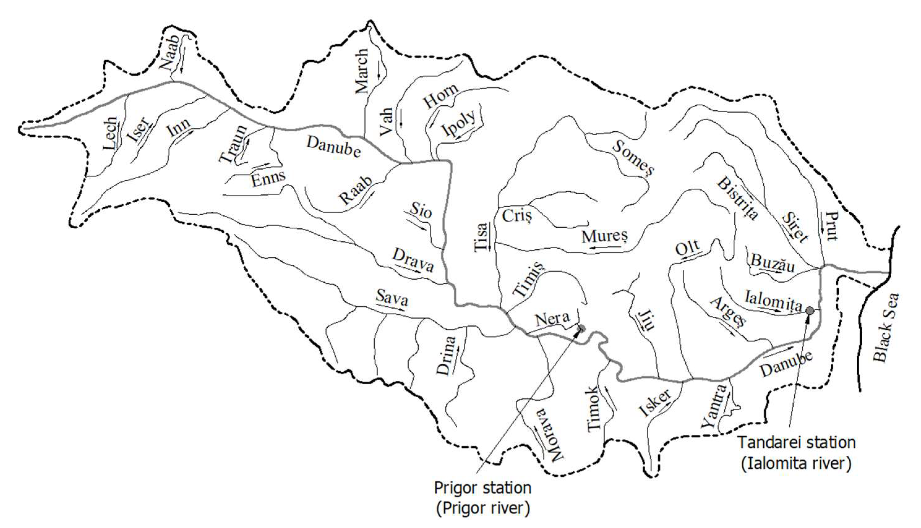
In this article, the maximum flows were determined for two rivers that have different origins of their maximum flows, through the MOM and L-moments, using statistical distributions suitable for Romania. The data series of maximum annual flows, according to Bulletin 17C [12], must have a minimum of 20 records. In the case of the Prigor river, the data series has a length of 21 records, and in the case of the Ialomita river, the data series has a length of 33 records.
Pearson III was chosen as the reference statistical distribution for the case studies. This was chosen for two reasons: the long-term use in Romania and the values close to the L-moments method with the MOM. The relative mean error (RME) and the relative absolute error (RAE) criteria [31] were used to compare the results, as well as the framing of the quantile values in the confidence interval of the reference distribution.
R M E = 1 n i = 1 n x i x p x i 2
R A E = 1 n i = 1 n x i x p x i
where n , x i , x p represent the sample size, the observed value and the estimated value for a given probability.
The results for the RME and RAE are presented in Table 7 and Table 8.
The validation of some distributions using these two criteria is not recommended, because they are determined by the differences only in the probability domain of the observed values, so it is recommended to approach validation with the criterion of the confidence interval for the MOM. The results of the performance indicators for L-moments were presented to note that their values were very small, but the significance was not valid.
For the Prigor river, where there is certainty of the natural registration of hydrometric data, the results were similar in the case of estimating the parameters with the MOM, with all distributions falling within the confidence interval of the reference distribution. For the L-moments method, all distributions fell within the confidence interval up to the probability of exceeding 0.1%, except for the GEV, which fell within 0.5%. Poor results for low probabilities are too influenced by small annual maximum flows in the case of a short data series [30].
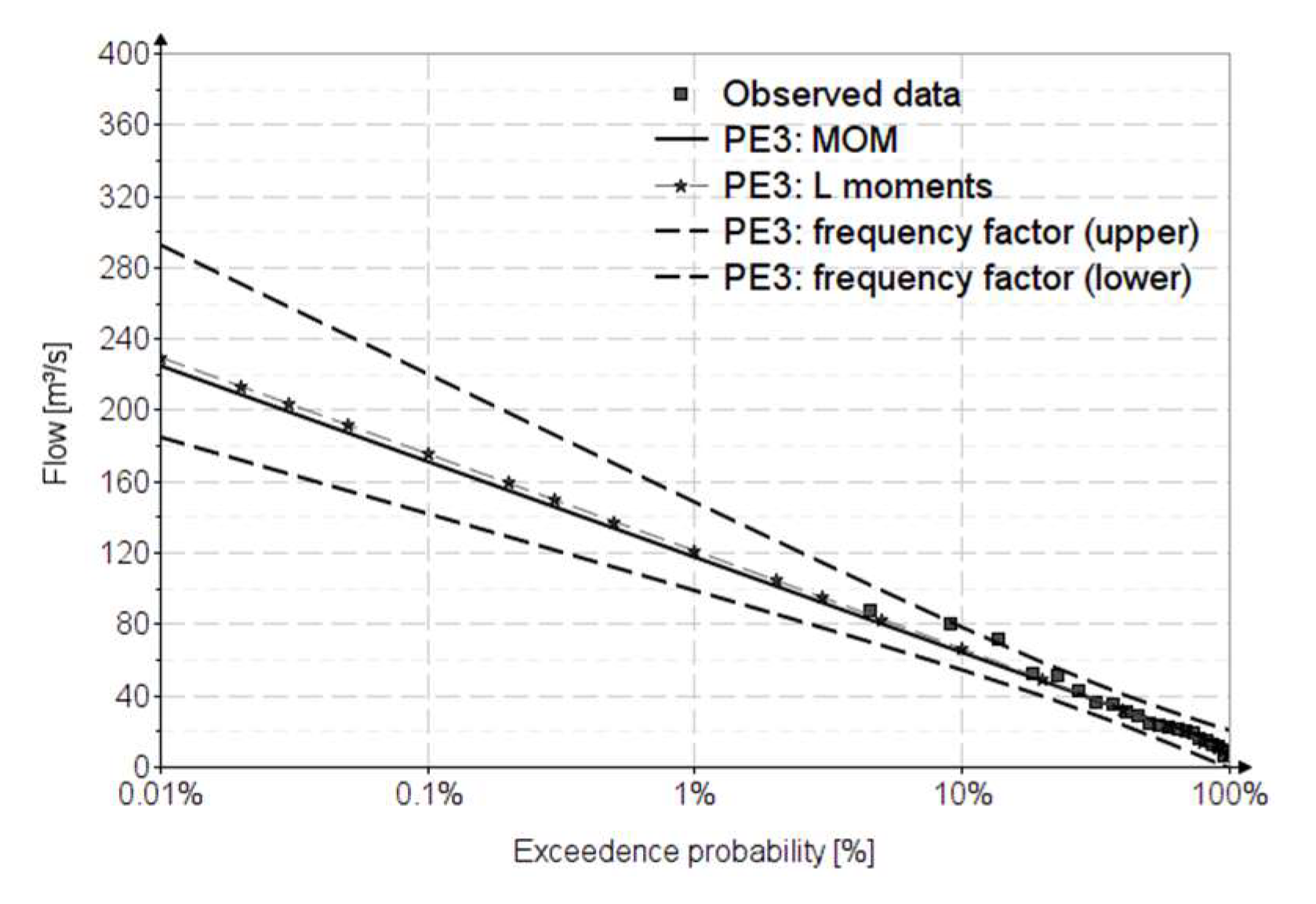
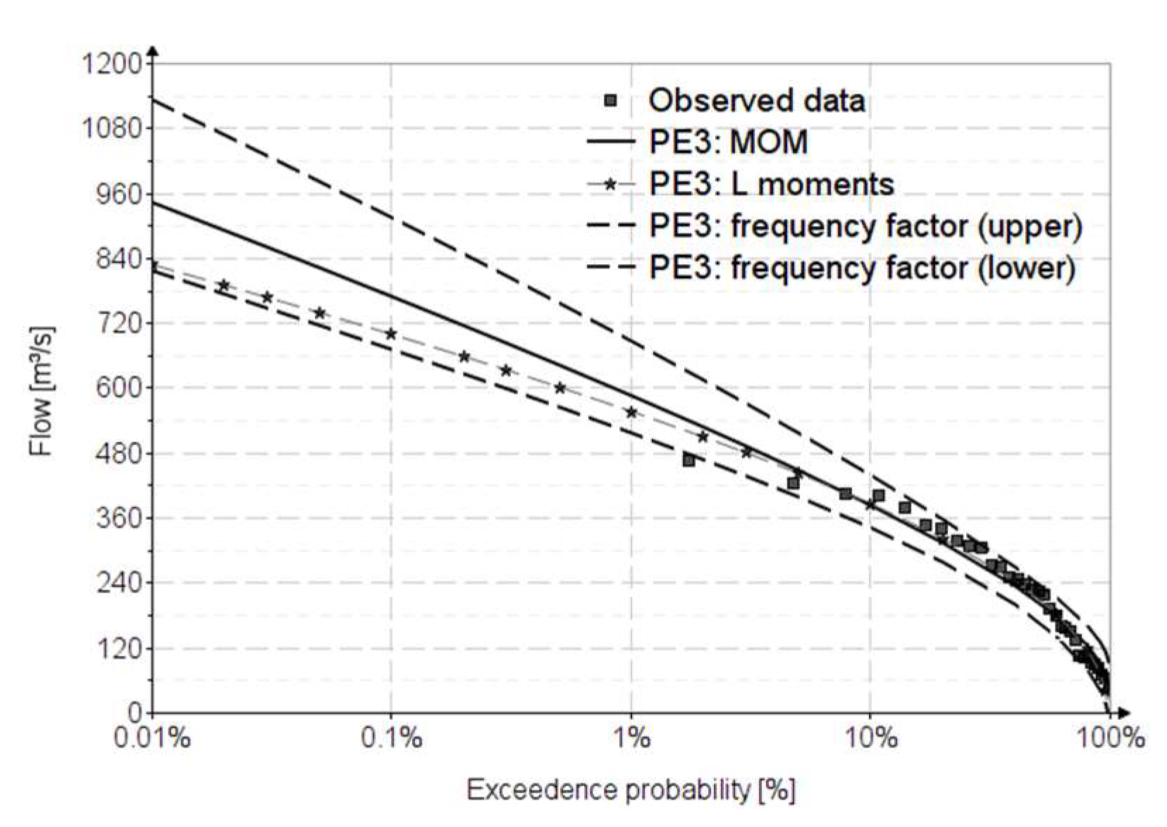
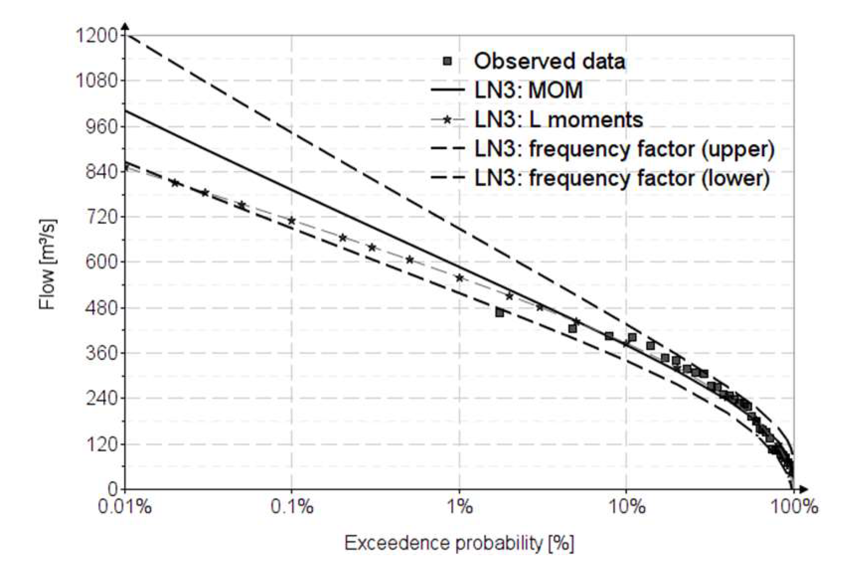
Figure 13 shows the statistical distributions analyzed compared to the chosen reference distribution for the Prigor case study.
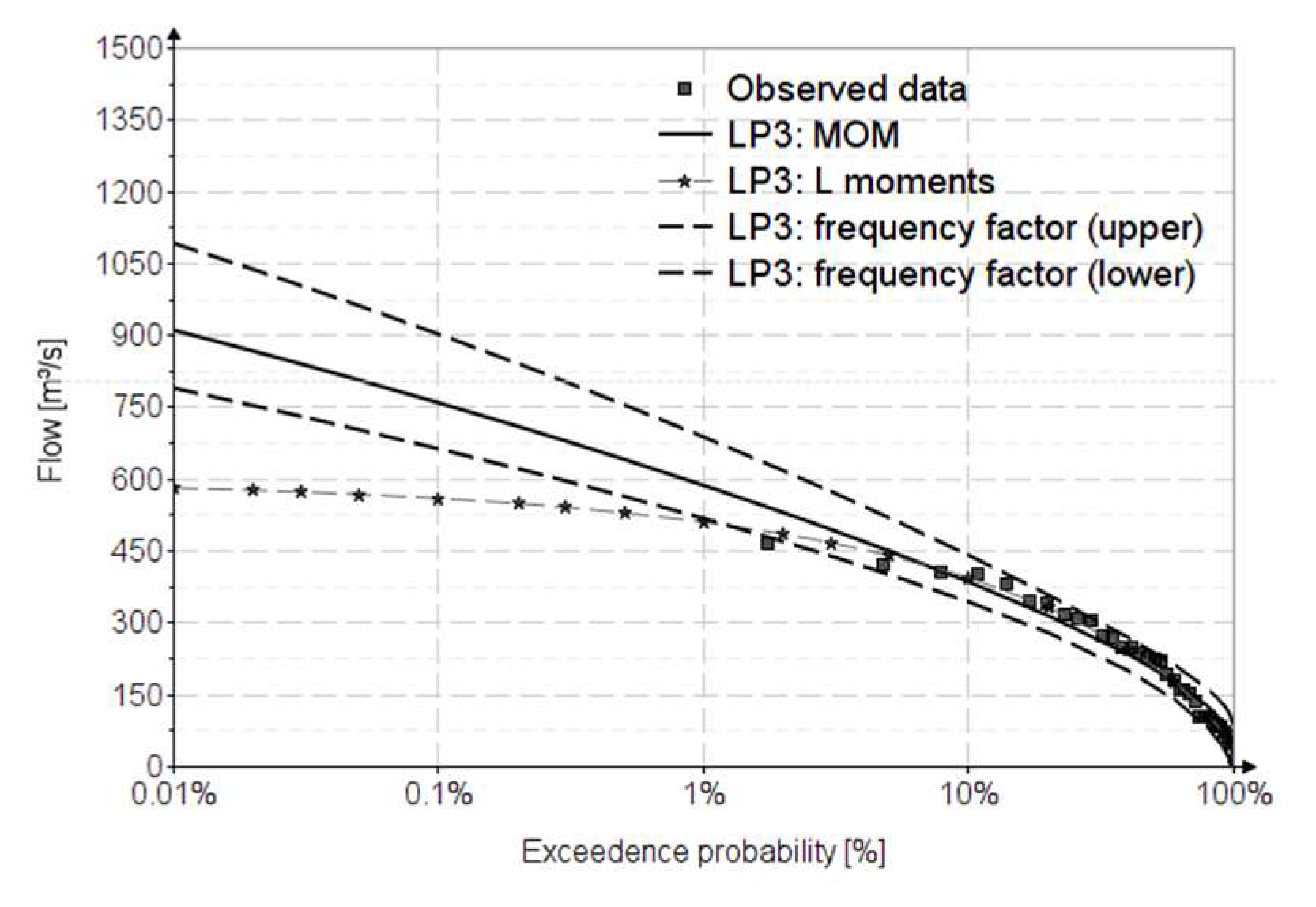
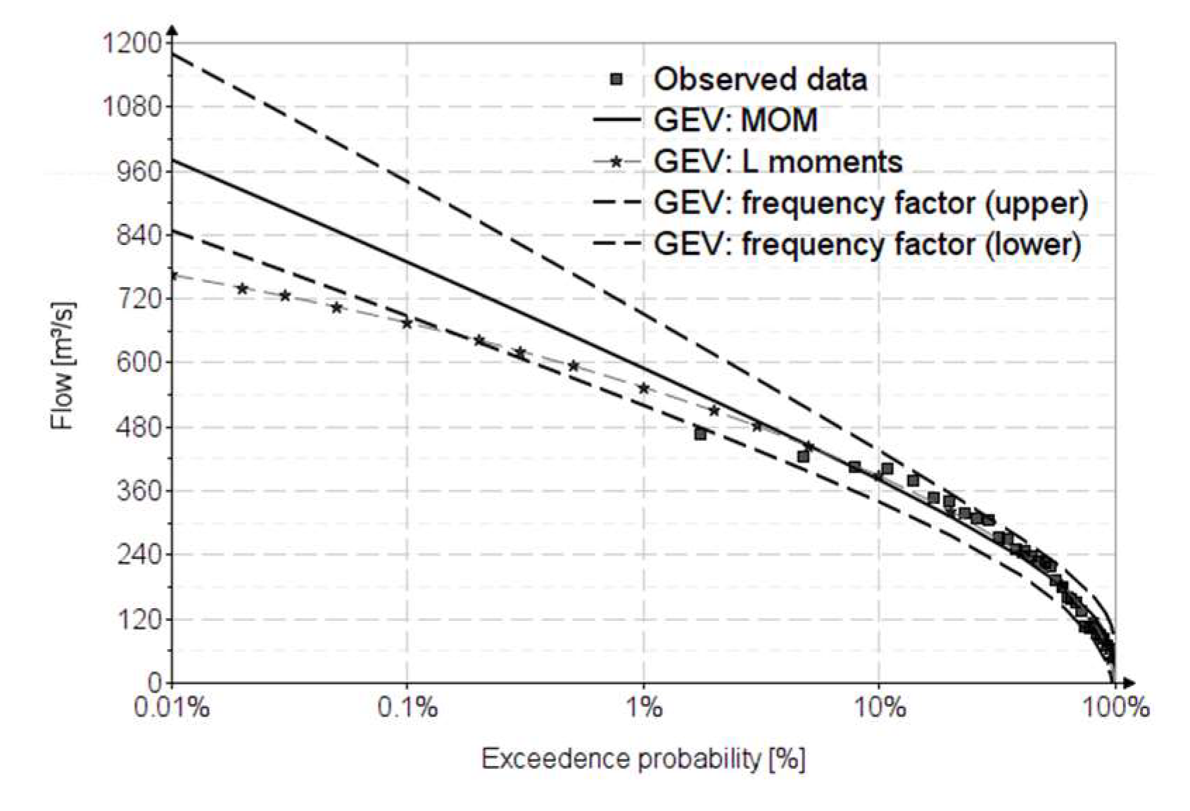
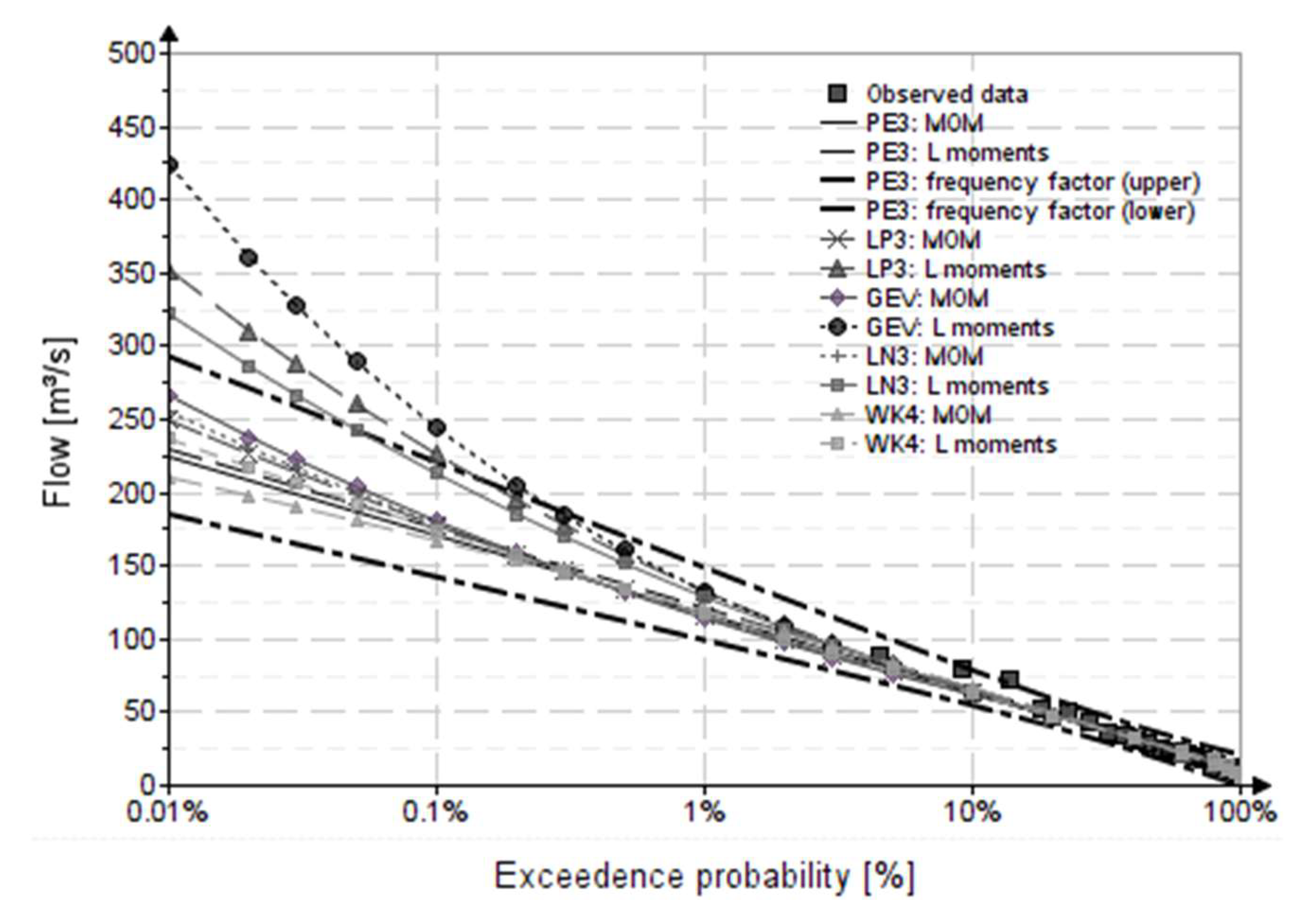
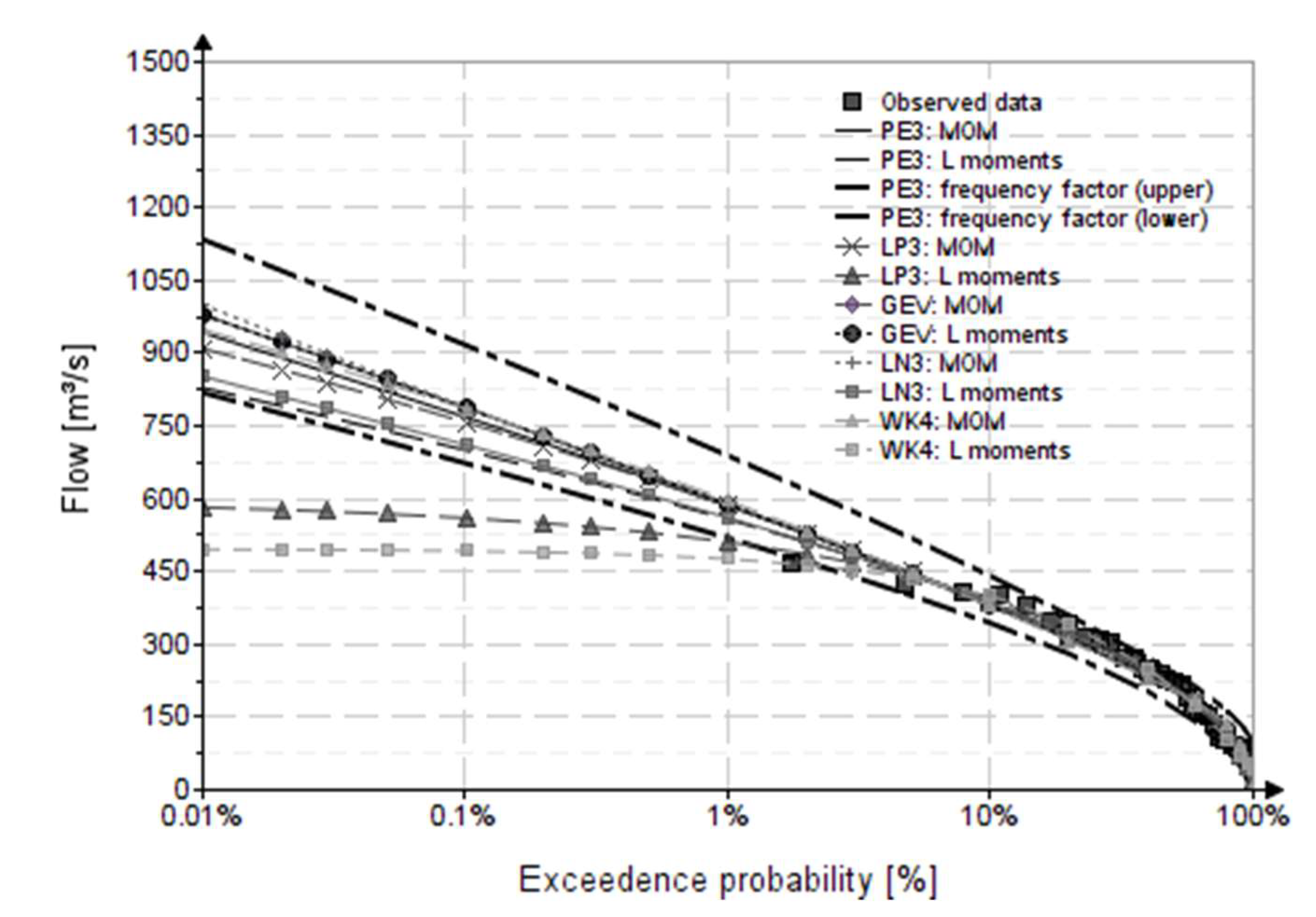
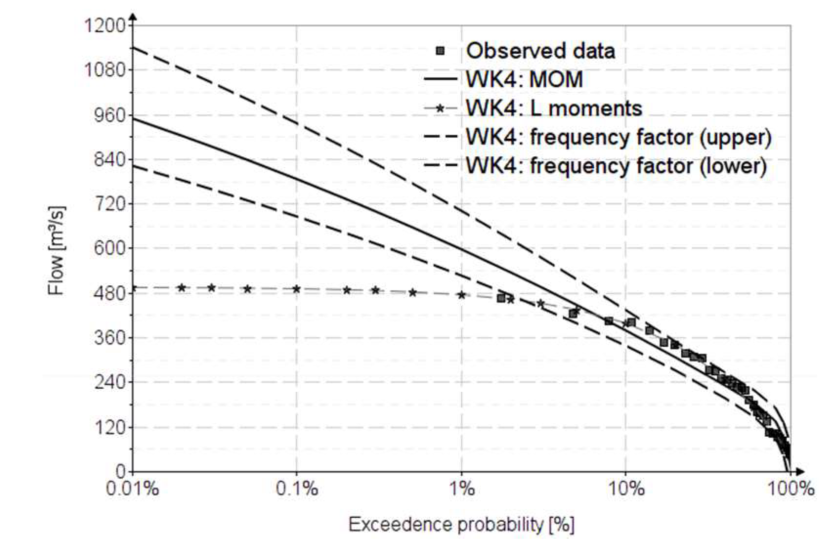
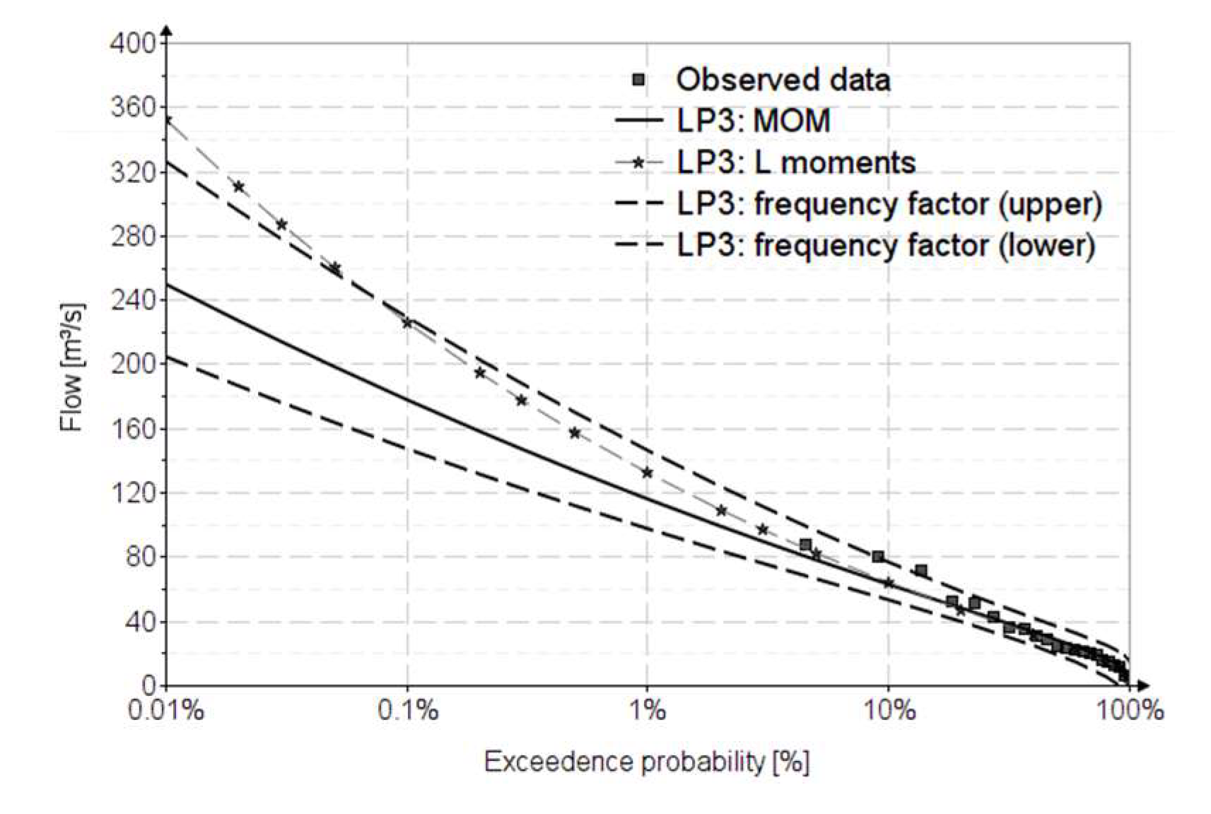
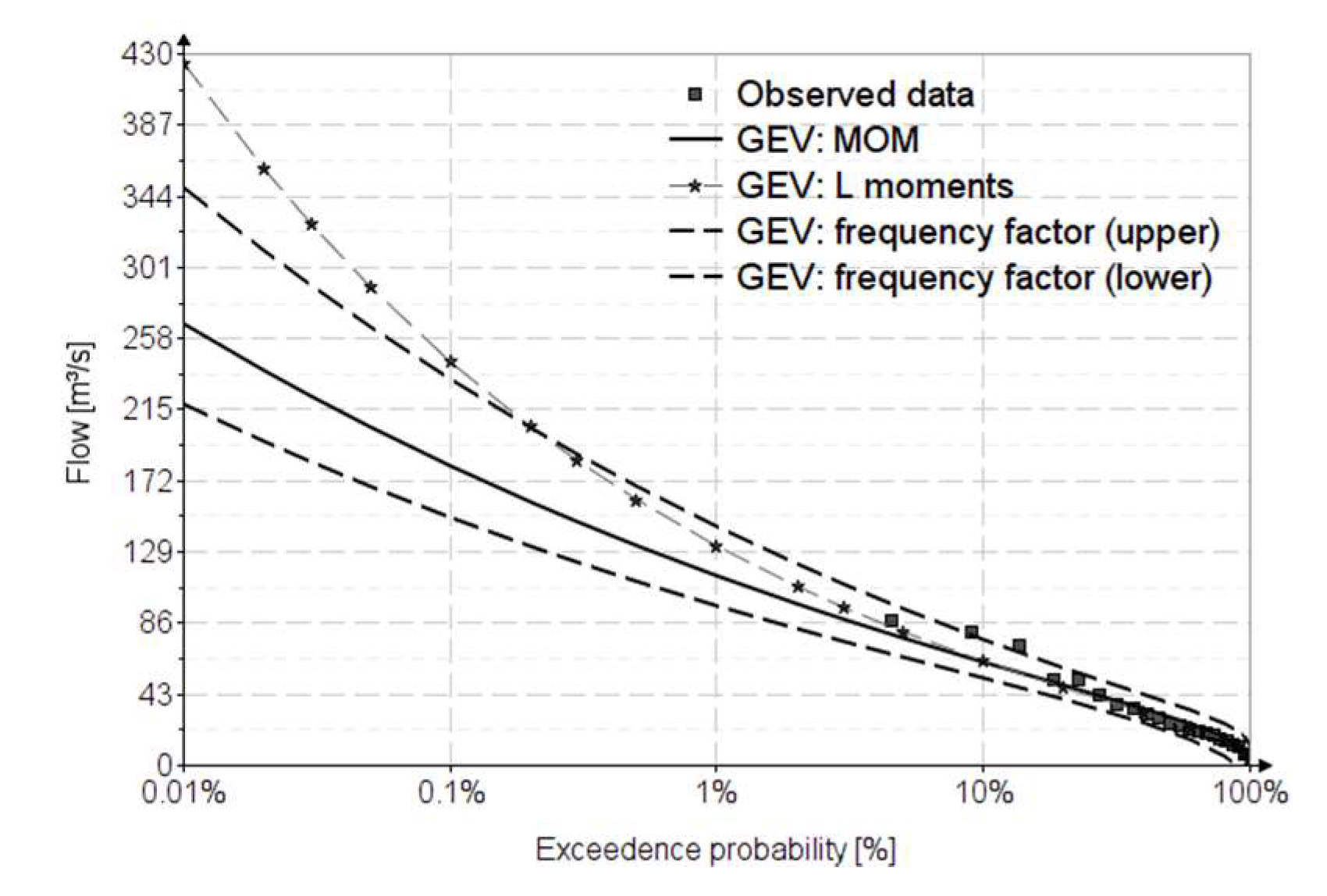
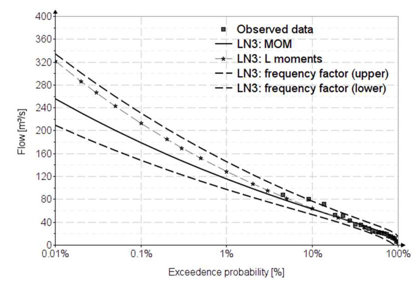
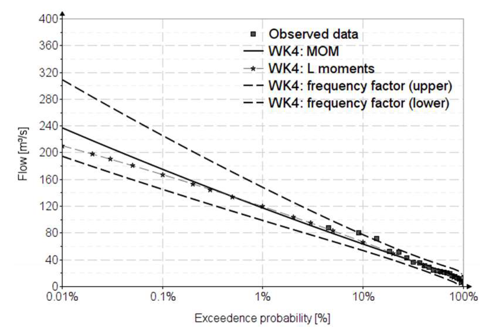
For the Ialomita river (Tandarei hydrometric station), the observed data were in the influenced regime, and the reconstruction of the data in the natural regime was with relatively large errors. In general, for large river basins and long river lengths, especially in low-altitude areas, there is also a high degree of natural attenuation of maximum flows. Furthermore, in this case, the results with the MOM were in accordance with NP 129/2011, all falling within the confidence interval of the reference distribution. For the L-moments method, the Wakeby, Log-Pearson and GEV distributions gave different shapes, possibly due to the high degree of attenuation of the maximum flows, with there being a threshold of the maximum values at low probabilities.
Figure 14 shows the statistical distributions analyzed compared to the chosen reference distribution for the Ialomita case study.
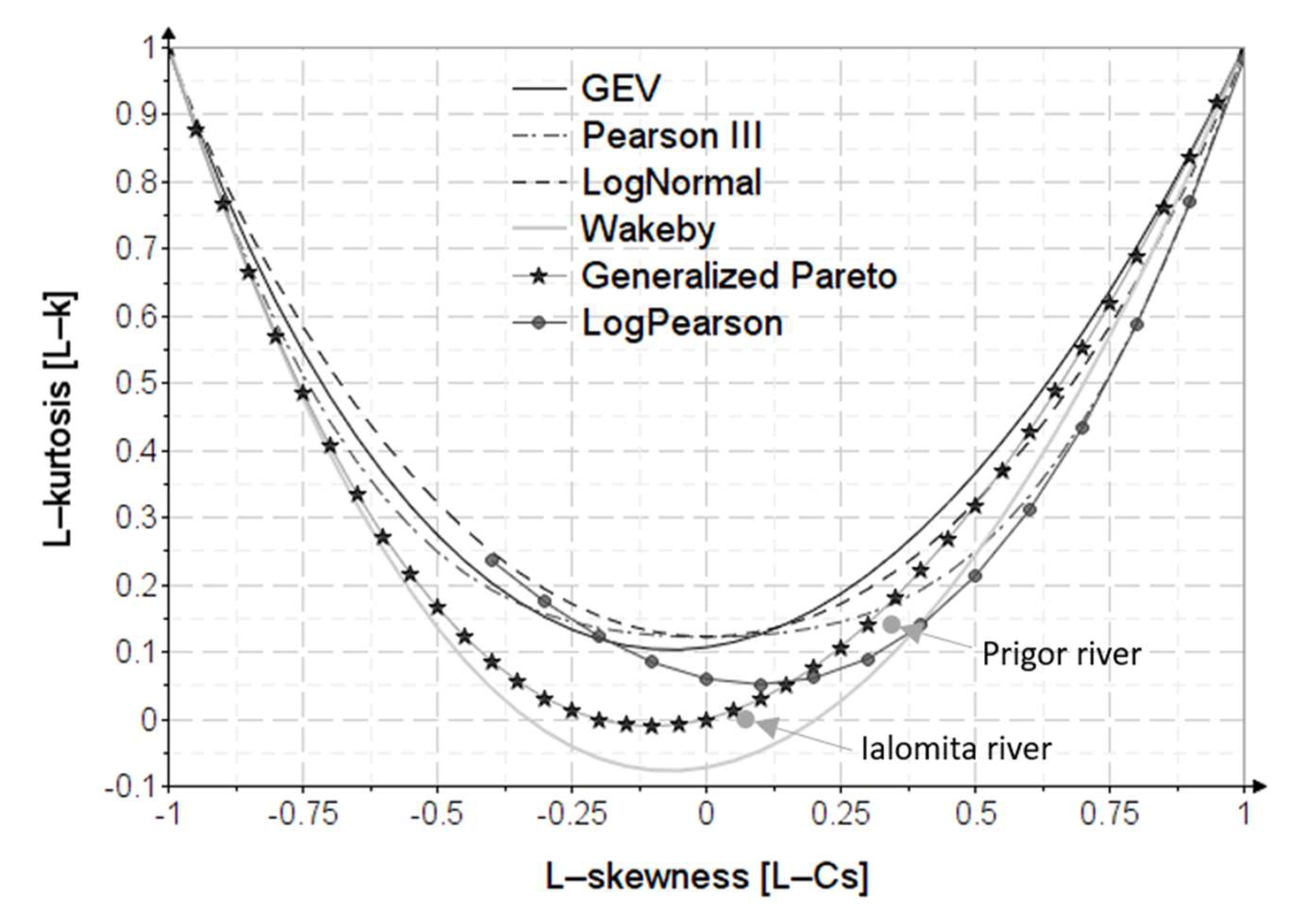
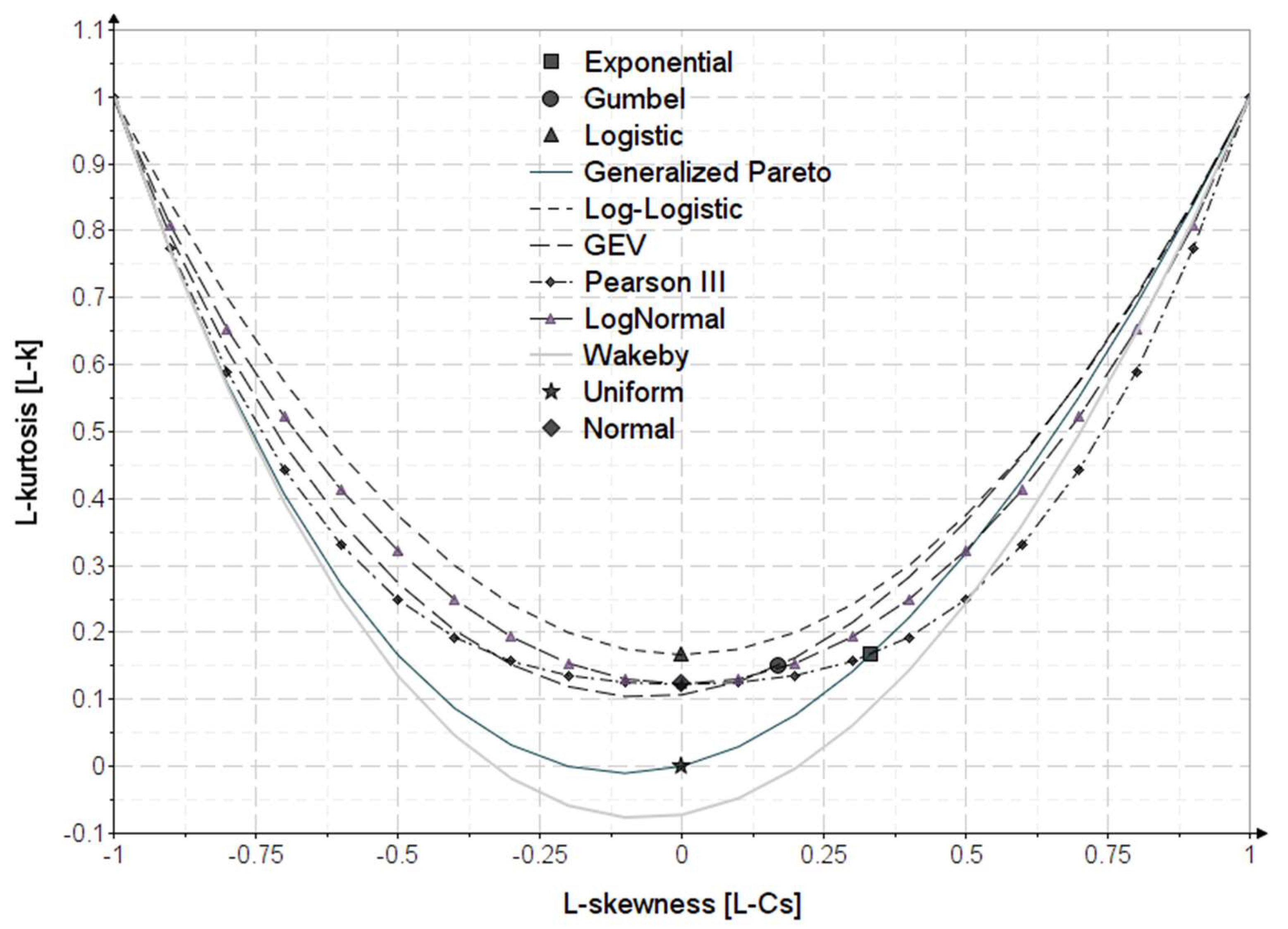
In the case of the Prigor river, the L-skewness (τ3) and L-kurtosis (τ4) values of the observed data did not differ much from those of the characteristic values of the τ4–τ3 variation of the analyzed theoretical distributions (Figure 15). Thus, all analyzed distributions had a similar graphic appearance.
The resulting values for τ3 and τ4 for the two rivers are presented in Table 9.
In the case of the Ialomita river, the τ3 and τ4 values of the observed data differed greatly from those of the characteristic values of the τ4–τ3 variation of the analyzed theoretical distributions. Thus, for the three-parameter distributions, with the calibration being done only as a function of τ3, the L-kurtosis τ4 took values consistent with the variation of τ4–τ3 of the theoretical distribution, disregarding the τ4 of the observed data, because for larger moments, they became unstable, making the resulting values unrealistic [32]. The Wakeby distribution is a distribution that was introduced in the flood frequency analysis in order to fulfil the “separation effect”, described by Matalas et al. 1975 [33], as much as possible, namely, to carry out an analysis so that the maximum flows were not excessively influenced by much of the small flows. The Wakeby distribution separates the right-hand side from the left-hand side of the distribution [33]. The Wakeby distribution has the property of a very thick left-hand tail (high flows) and a right-hand tail that is thick (small flow) enough to decrease the average skew [33], which makes the middle part of the distribution steeper than traditional skewed curves.
In the case of the four-parameter Wakeby distribution, the resulting values of the parameters matched those of a particular case of the distribution, namely, the generalized Pareto [17]. Thus, in the particular case of the Ialomita river dataset, the Wakeby distribution turned into the generalized Pareto distribution, which has the expression of the quantile function, as follows:
x ( p ) = γ + β α 1 p α
The term on the right of the Wakeby quantile has a constant value of −40.9 m3/s, which, due to the “–“ sign in front of the term, acquires positive values. The value of this term represents the value of the position parameter γ from the Pareto quantile, with the rest of the terms remaining unchanged. It can also be seen on the graph that the value of τ4 corresponding to τ3 is that of the particular Wakeby distribution, namely, the generalized Pareto, respecting the τ4 of the observed data.
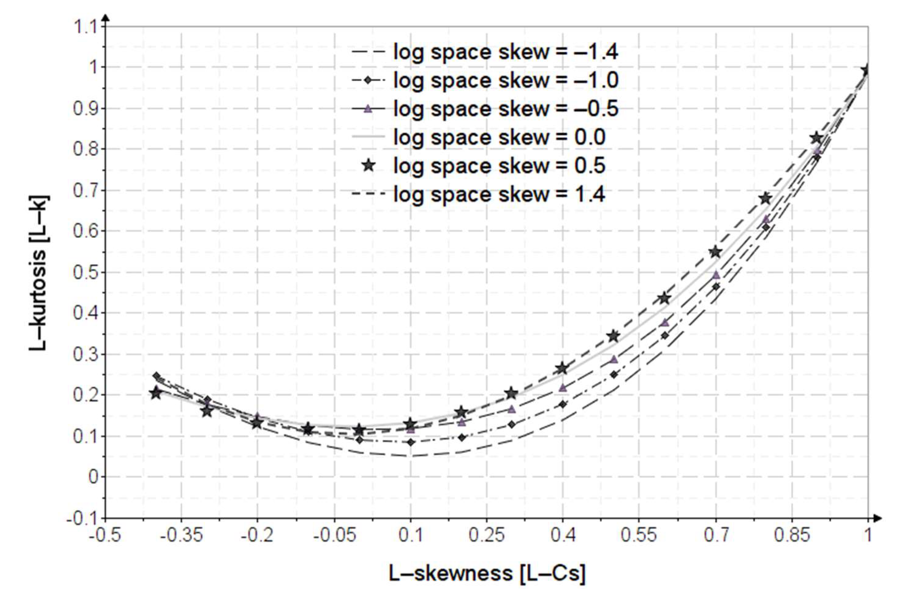
In the case of the Log-Pearson distribution, calculated based on the moments obtained from the density function, it had a similar appearance to the Wakeby distribution, but the latter had, in some cases, better results [32]. The τ4–τ3 variation in the case of the LogPearson (Figure 16) distribution was varied depending on the asymmetry values in the log space [34].
The graphs between τ3 and τ4 also represent a criterion for choosing the best distributions to use in achieving a regionalization based on L-moments [5,17].

7. Conclusions

This article briefly described the most used statistical distributions for the maximum discharge and the latest methods for estimating the distribution parameters using engineering mathematical software.
The use of the Pearson III distribution in Romania must be maintained for the MOM, because the estimation of the parameters was simple and gave good results. A statistical distribution that can be a good alternative to Pearson III is LogNormal (LN3), being the most widely used distribution in Europe for maximum flows [10,24].
The introduction of other statistical distributions should be done after the regionalization studies are conducted, and it should be a simpler alternative, if this proves to be the case.
The method of estimating the parameters must remain the method of ordinary moments, because it has proven to be effective for Romania. The adoption of other estimation methods (L-moments) is useful but requires a long transition period, in which the two methods must be used in parallel.
In the regulations for calculating the maximum flows, it is recommended that statistical distributions should be presented in full, i.e., the functions of density, distribution and quantile, where they exist, as well as the inclusion of computer applications for estimating the parameters of statistical distributions and calculation examples.
The calibration of the three-parameter distributions is easy with the method of ordinary moments. Since asymmetry does not characterize short data strings, it is generally correct, highlighting two methods. A method of correcting the asymmetry according to the genesis of the data was presented in this article, which is based on choosing the asymmetry as a multiple of the coefficient of variation. Another method is to use skewness correction coefficients depending on the relatively short length of the observed data string. A disadvantage of this method is that it is not possible to calibrate the kurtosis function (non-linear function), because it has large differences for a sample compared to that of a population.
The L-moments for the samples were very close to those of the population; thus, no correction of τ3 and τ4 was necessary, being thus more robust and less influenced by the effects of sampling variability [5] due to the fact that the L-moments are linear functions. The use of a four-parameter distribution allows calibration as a function of τ3 and τ4, which is an advantage in achieving a regionalization based on L-moments.

Author Contributions

Conceptualization, C.I. and C.G.A.; methodology, C.I. and C.G.A.; software, C.I. and C.G.A.; validation, C.I. and C.G.A.; formal analysis, C.I. and C.G.A.; investigation, C.I. and C.G.A.; resources, C.I. and C.G.A.; data curation, C.I. and C.G.A.; writing—original draft preparation, C.I. and C.G.A.; writing—review and editing, C.I. and C.G.A.; visualization, C.I. and C.G.A.; supervision, C.I. and C.G.A.; project administration, C.I. and C.G.A.; funding acquisition, C.I. and C.G.A. All authors have read and agreed to the published version of the manuscript.

Funding

This research received no external funding.

Institutional Review Board Statement

Not applicable.

Informed Consent Statement

Not applicable.

Data Availability Statement

Not applicable.

Conflicts of Interest

The authors declare no conflict of interest.

Abbreviations

AMannual maximum
POTpeaks-over-threshold
MOMmethod of ordinary moments
L-momentsrepresent a method of parameters estimation; in Table 3 and Table 6, they are noted with L.
μ expected value; arithmetic mean
σ standard deviation
CVcoefficient of variation
CScoefficient of skewness; skewness
L-CVcoefficient of variation based on the L-moments method
L-CScoefficient of skewness based on the L-moments method
PE3Pearson III distribution
GEVgeneralized extreme value distribution
LP3Log-Pearson III distribution
LN3LogNormal with a three-parameters distribution
WK4four-parameters Wakeby distribution
ξ coefficient chosen depending on the origin of the flows
FPEGDfour-parameter exponential gamma distribution
f(x)probability density function
F(x)complementary cumulative distribution function
x(p)quantile function; p represents the exceedance probability.
RAErelative absolute error
RMErelative mean error

Appendix A. The Formula for Sample L-Moments

For calculating the sample L-moments, the observed data, x i , must be in ascending order.
The sample L-moments are:
L 1 = b 0 first   L - moment
L 2 = 2 b 1 b 0 second   L - moment
L 3 = 6 b 2 6 b 1 + b 0 third   L - moment
L 4 = 20 b 3 30 b 2 + 12 b 1 b 0 fourth   L - moment
where b 0 , b 1 , b 2 , b 3 represent natural estimators, expressed as b 0 = 1 n i = 1 n x i
b 1 = 1 n i = 1 n x i i 1 n 1
b 2 = 1 n i = 1 n x i i 1 n 1 i 2 n 2
b 3 = 1 n i = 1 n x i i 1 n 1 i 2 n 2 i 3 n 3
where n is the length of th data series.
Using the L-moments, the coefficients of variation, ( τ 2 ), skewness ( τ 3 ) and kurtosis ( τ 4 ) are defined as [4,16]:
τ 2 = L 2 L 1 , which is the L-CV;
τ 3 = L 3 L 2 , which is the L-Skewness;
τ 4 = L 4 L 2 , which is the L-Kurtosis
Figure A1 shows the variation of kurtosis (excess) depending on the skewness [16], obtained with the L-moments method, for certain theoretical distributions often used in hydrology and in this article.
Figure A1. The variation of L-kurtosis–L-skewness.
Water 14 02884 g0a1

Appendix B. The First Four Raw Moments for the Wakeby Distribution

The first four raw moments of the WK4 distribution are:
m 1 = α β + 1 γ δ 1
m 2 = 2 α 2 β + 1 2 β + 1 2 γ 2 α δ 2 β + 1 γ + 2 α β + 5 α δ + β 2 + 2 β + 1 γ + α β + 2 α β + 1 δ β + 1 δ 1 2 δ 1
m 3 = 3 · α 3 ( β + 1 ) · ( 2 · β + 1 ) · ( 3 · β + 1 ) 6 · γ [ ( β + 1 ) · ( 2 · β + 1 ) · ( δ 2 · β 1 ) · ( δ β 1 ) · ( δ 1 ) · ( 2 · δ β 1 ) · ( 2 · δ 1 ) · ( 3 · δ 1 ) ] · [ 12 · α · δ 5 δ 4 · [ γ · ( 12 · α · β + 6 · α ) + 42 · α 2 · β + 52 · α 2 ] + δ 3 · [ γ 2 · ( 4 · β 2 + 6 · β + 2 ) + α · γ · ( 2 · β + 1 ) · ( 21 · β + 26 ) + α 2 · ( 42 · β 2 + 143 · β + 91 ) ] { δ 2 · [ γ 2 · ( 14 · β 3 + 31 · β 2 + 22 · β + 5 ) + α · γ · ( 2 · β + 1 ) · ( 21 · β 2 + 61 · β + 35 ) + α 2 · ( 12 · β 3 + 83 · β 2 + 151 · β + 70 ) ] + δ · [ γ 2 · ( β + 1 ) 2 · ( 2 · β + 1 ) · ( 7 · β + 4 ) + α · γ · ( 2 · β + 1 ) · ( 6 · β 3 + 28 · β 2 + 45 · β + 18 ) + ] α 2 · ( 10 · β 3 + 47 · β 2 + 63 · β + 24 ) ] γ 2 · ( β + 1 ) 3 · ( 2 · β + 1 ) 2 α · γ · ( 2 · β + 1 ) 2 · ( β 3 + 3 · β + 3 ) α 2 · ( β + 1 ) · ( 2 · β 2 + 6 · β + 3 ) )
m 4 = 24 · γ 4 ( δ 1 ) · ( 2 · δ 1 ) · ( 3 · δ 1 ) · ( 4 · δ 1 ) 24 · α · γ 3 · ( 3 · δ β 2 ) · ( 2 · δ 2 δ · ( 3 · β + 6 ) + β 2 + 2 · β + 2 ) ( β + 1 ) · ( δ β 1 ) · ( δ 1 ) · ( 2 · δ β 1 ) · ( 2 · δ 1 ) ( 3 · δ β 1 ) · ( 3 · δ 1 ) + 24 · α 2 · γ 2 · [ 4 · δ 4 δ 3 · ( 18 · β + 18 ) + δ 2 · ( 28 · β 2 + 66 · β + 33 ) δ · ( 18 · β 3 + 66 · β 2 + 72 · β + 24 ) + 4 · β 4 + 18 · β 3 + 33 · β 2 + 24 · β + 6 ] ( β + 1 ) · ( 2 · β + 1 ) · ( δ 2 · β 1 ) · ( δ β 1 ) · ( δ 1 ) · ( 2 · δ 2 · β 1 ) · ( 2 · δ β 1 ) · ( 2 · δ 1 ) 24 · α 3 · γ · ( δ 3 · β 2 ) · ( δ 2 δ · ( 3 · β + 2 ) + 2 · β 2 + 6 · β + 2 ) ( β + 1 ) · ( 2 · β + 1 ) · ( 3 · β + 1 ) · ( δ 3 · β 1 ) ( δ 2 · β 1 ) · ( δ β 1 ) ( δ 1 ) + 24 · α 4 ( β + 1 ) · ( 2 · β + 1 ) · ( 3 · β + 1 ) · ( 4 · β + 1 )
The skewness ( γ 1 ) and kurtosis ( γ 2 ) are obtained from the formulas presented in Section 3.1.

Appendix C. Built-In Function Din Mathcad

Γ x returns the value of the Euler gamma function of x;
Γ α , x returns the value of the incomplete gamma function of x with parameter a;
d g a m m a x , s returns the probability density for value x, for the Gamma distribution;
p g a m m a x , s returns the cumulative probability distribution for value x, for the Gamma distribution;
q g a m m a p , s returns the inverse cumulative probability distribution for probability p, for the Gamma distribution;
d n o r m x , α , β returns the probability density for value x, for the Normal distribution;
p n o r m x , α , β returns the cumulative probability distribution for value x, for the Normal distribution;
q n o r m p , 0 , 1 returns the inverse standard cumulative probability distribution for probability p, for the Normal distribution;
c n o r m x returns the cumulative probability distribution with mean 0 and variance 1, for the Normal distribution;
d l n o r m x , α , β returns the probability density for value x, for the LogNormal distribution;
p l n o r m x , α , β returns the cumulative probability distribution for value x, for the LogNormal distribution;
q l n o r m p , μ , σ returns the inverse cumulative probability distribution for probability p, for thee LogNormal distribution;
p c h i s q x , d returns the cumulative probability distribution for value x, for the Chi-Squared distribution;
q c h i s q p , d returns the inverse cumulative probability distribution for probability p, for the Chi-Squared distribution;
e r f x returns the error function;
i b e t a a , x , y , the incomplete Beta function, returns the value of the incomplete beta function of x and y with parameter a .

References

  1. STAS 4068/1-82; Maximum Water Discharges and Volumes, Determination of maximum Water Discharges and Volumes of Watercourses. The Romanian Standardization Institute: Bucharest, Romania, 1982.
  2. STAS 4273-83; Hydrotechnical Constructions, Classification in the Importance Class. The Romanian Standardization Institute: Bucharest, Romania, 1983.
  3. Ardiclioglu, M.; Hadi, A.M.W.M.; Periku, E.; Kuriqi, A. Experimental and Numerical Investigation of Bridge Configuration Effect on Hydraulic Regime. Int. J. Civ. Eng. 2022, 20, 981–991. [Google Scholar] [CrossRef]
  4. The Regulations Regarding the Establishment of Maximum Flows and Volumes for the Calculation of Hydrotechnical Retention Constructions; Indicative NP 129-2011; Ministry of Regional Development and Tourism: Bucharest, Romania, 2012.
  5. Hosking, J.R.M. L-moments: Analysis and Estimation of Distributions using Linear, Combinations of Order Statistics. J. R. Statist. Soc. 1990, 52, 105–124. [Google Scholar] [CrossRef]
  6. Gubareva, T.S.; Gartsman, B.I. Estimating Distribution Parameters of Extreme Hydrometeorological Characteristics by L-Moment Method. Water Resour. 2010, 37, 437–445. [Google Scholar] [CrossRef]
  7. Lang, M.; Ouarda, T.B.M.J.; Bobee, B. Towards operational guidelines for over-threshold modeling. J. Hydrol. 1999, 225, 103–117. [Google Scholar] [CrossRef]
  8. Keast, D.; Ellison, J. Magnitude Frequency Analysis of Small Floods Using the Annual and Partial Series. Water 2013, 5, 1816–1829. [Google Scholar] [CrossRef]
  9. Goda, Y.; Kudaka, M.; Kawai, H. Incorporation of Weibull distribution in L-moments method for regional frequency analysis of peaks-over-threshold wave heights. In Proceedings of the 32nd Conference on Coastal Engineering 2010, Shanghai, China, 30 June–5 July 2010. [Google Scholar]
  10. World Meteorological Organization. (WMO-No.718) 1989 Statistical Distributions for Flood Frequency Analysis; Operational Hydrology Report no. 33; WHO: Geneva, Switzerland, 1989. [Google Scholar]
  11. Bulletin 17B Guidelines for determining Flood Flow Frequency; Hydrology Subcommittee, Interagency Advisory Committee on Water Data, U.S. Departament of the Interior, U.S. Geological Survey, Office of Water Data Coordination: Reston, VA, USA, 1981.
  12. Bulletin 17C Guidelines for determining Flood Flow, Frequency; U.S. Department of the Interior, U.S. Geological Survey: Reston, VA, USA, 2017.
  13. Diacon, C.; Serban, P. Hydrological Syntheses and Regionalizations; Technical Publishing House: Bucharest, Romania, 1994. [Google Scholar]
  14. Mandru, R.; Ioanitoaia, H. Ameliorative Hydrology; Agro-Silvica Publishing House: Bucharest, Romania, 1962. [Google Scholar]
  15. Constantinescu, M.; Golstein, M.; Haram, V.; Solomon, S. Hydrology; Technical Publishing House: Bucharest, Romania, 1956. [Google Scholar]
  16. Singh, V.P. Entropy-Based Parameter Estimation in Hydrology; Springer: Dordrecht, The Netherlands, 1998; ISBN1 978-90-481-5089-2. ISBN2 978-94-017-1431-0. [Google Scholar] [CrossRef]
  17. Rao, A.R.; Hamed, K.H. Flood Frequency Analysis; CRC Press: Boca Raton, FL, USA, 2000. [Google Scholar]
  18. Grimaldi, S.; Kao, S.-C.; Castellarin, A.; Papalexiou, S.-M.; Viglione, A.; Laio, F.; Aksoy, H.; Gedikli, A. Statistical Hydrology. In Treatise on Water Science; Elsevier: Oxford, UK, 2011; Volume 2, pp. 479–517. [Google Scholar]
  19. Chow, V.T.; Maidment, D.R.; Mays, L.W. Applied Hydrology; McGraw-Hill, Inc.: New York, NY, USA, 1988; ISBN 007-010810-2. [Google Scholar]
  20. Song, S.; Song, X.; Kang, Y. Entropy-Based Parameter Estimation for the Four-Parameter Exponential Gamma Distribution. Entropy 2017, 19, 189. [Google Scholar] [CrossRef]
  21. Dey, S.; Al-Zahrani, B.; Basloom, S. Dagum Distribution: Properties and Different Methods of Estimation. Int. J. Stat. Probab. 2017, 6, 74–92. [Google Scholar] [CrossRef]
  22. Ehab, E.A.; Soaad, A.; Nahed, T.A. A new alpha power Ibrahim distribution: Properties and applications. Sohag J. Jr. Sci. Res. 2021. [Google Scholar]
  23. World Meteorological Organization. (WMO-No.233) Estimation of Maximum Floods; Technical Note no. 98; WHO: Geneva, Switzerland, 1969. [Google Scholar]
  24. McMahon, T.A.; Arenas, A.D. UNESCO Methods of computation of low streamflow. In Studies and Reports in Hydrology; UNESCO: Paris, France, 1982; ISBN 92-102013-7. [Google Scholar]
  25. EM 1110-2-1415 Hydrologic Frequency Analysis, Engineering and Design; Department of the Army U.S. Army Corps of Engineers: Washington, DC, USA, 1993.
  26. IASH-Unesco-WMO; AIHS-Unesco-OMM. Floods and Their Computation: Proceedings of the Leningrad Symposium; The International Association of Scientific Hydrology: Gentbrugge, Belgium, 1969. [Google Scholar]
  27. Cudworth, A.G., Jr. Flood Hydrology Manual; United States Department of the Interior Bureau of Reclamation: Washington, DC, USA, 1989. [Google Scholar]
  28. The Romanian Water Classification Atlas, Part I–Morpho-Hydrographic Data on the Surface Hydrographic Network; Ministry of the Environment: Bucharest, Romania, 1992.
  29. Nguyen, V.T.V.; In-Na, N. Plotting formula for Pearson Type III distribution considering histotical information. Environ. Monit. Assess. 1992, 23, 137–152. [Google Scholar] [CrossRef] [PubMed]
  30. Wang, Q.J. LH moments for statistical analysis of extreme events. Water Resour. Res. 1997, 33, 2841–2848. [Google Scholar] [CrossRef]
  31. Singh, K.; Singh, V.P. Parameter Estimation for Log-Pearson Type III Distribution by Pome. 1988. Available online: https://hdl.handle.net/1969.1/164673 (accessed on 7 July 2022).
  32. Rao, A.R.; Arora, P.S. An Empirical Study of Probability Distributions Of Annual Maximum Floods. In Hydrologic Frequency Modeling; Springer: Dordrecht, The Netherlands, 1987. [Google Scholar]
  33. Houghton, C. Birth of a Parent: The Wakeby Distribution for Modeling Flood Flows; Working Paper no. MIT-EL77-033WP; Water Resources Research: Tucson, AZ, USA, 1978; Volume 14, Issue 6. [Google Scholar]
  34. Griffis, V.W.; Asce, M.; Stedinger, J.R. Log-Pearson Type 3 Distribution and Its Application in Flood Frequency Analysis. I: Distribution Characteristics. J. Hydrol. Eng. 2007, 12, 492–500. [Google Scholar] [CrossRef]
Figure 1. Methodological approach.
Water 14 02884 g001
Figure 2. Location map of Study areas: Prigor and Ialomita rivers, Romania.
Water 14 02884 g002
Figure 3. Pearson III distribution.
Water 14 02884 g003
Figure 4. LogPearson III distribution.
Water 14 02884 g004
Figure 5. GEV distribution.
Water 14 02884 g005
Figure 6. LogNormal distribution.
Water 14 02884 g006
Figure 7. Wakeby distribution.
Water 14 02884 g007
Figure 8. Pearson III distribution.
Water 14 02884 g008
Figure 9. LogPearson III distribution.
Water 14 02884 g009
Figure 10. GEV distribution.
Water 14 02884 g010
Figure 11. LogNormal distribution.
Water 14 02884 g011
Figure 12. Wakeby distribution.
Water 14 02884 g012
Figure 13. Comparing the frequency distributions for the Prigor river.
Water 14 02884 g013
Figure 14. Comparing the frequency distributions for the Ialomita river.
Water 14 02884 g014
Figure 15. The variation of L-kurtosis–L-skewness with the sample data value of L-kurtosis and L-skewness.
Water 14 02884 g015
Figure 16. The variation of the L-kurtosis–L-skewness, for LogPearson.
Water 14 02884 g016
Table 1. Observed data from the Tandarei station.
Data[yr]19761977197819791980198119821983198419851986
Flow[m3/s]22013615238140127315940534616189
Data[yr]19871988198919901991199219931994199519961997
Flow[m3/s]10630847.565.33068522872224317424
Data[yr]19981999200020012002200320042005200620072008
Flow[m3/s]34118094.5270192103251468237249104
Table 2. Parameter estimates by the MOM and L-moments.
Frequency DistributionMOML-Moments
α β γ δ α β γ δ
Pearson III3.60262.20-13.3633.6−224.2-
LogPearson18.243−0.1317.65-2.852−0.412−6.396-
GEV0.01593.8171-0.129110173.2-
LogNormal5.8010.329−124-6.480.183−440.7-
Wakeby1170.0631187−9.493.06 × 1020.6723.8 × 1011−8.5 × 10⁹
Table 3. Comparison of the estimated values for the usual probability for the Ialomita river.
PFrequency Distributions
Pearson IIILogPearsonGEVLogNormalWakeby
MOMLMOMLMOMLMOMLMOML
[%][m3/s][m3/s][m3/s][m3/s][m3/s][m3/s][m3/s][m3/s][m3/s][m3/s]
0.01941828909582979765999851948495
0.1768699757560787675789711785492
1585557585511588554586560596475
5446443448441443444443443446435
40233244232247234244234244230250
80123118123111126119126120136104
9570.143.172.549.167.543.567.442.854.356.3
Table 4. Observed data from the Prigor station.
Data[yr]20002001200220032004200520062007200820092010
Flow[m3/s]3519.922.111.680.38851.672.216.242.628.5
Data[yr]2011201220132014201520162017201820192020
Flow[m3/s]12.831.224.152.220.218.96.4924.91536.6
Table 5. Parameter estimates by the MOM and L-moments.
Frequency DistributionMOML-Moments
α β γ δ α β γ δ
Pearson III0.96423.411.3-1.13923.17.5-
LogPearson187−0.04712.1-34610.012−36.6-
GEV−0.11215.123.3-−0.21014.321.9-
LogNormal3.4820.559−4.13-3.350.654−1.27-
Wakeby29923.721.10.03377645326.7−0.044
Table 6. Comparison of the estimated values for usual probability for the Prigor river.
PFrequency Distributions
Pearson IIILogPearsonGEVLogNormalWakeby
MOMLMOMLMOMLMOMLMOML
[%][m3/s][m3/s][m3/s][m3/s][m3/s][m3/s][m3/s][m3/s][m3/s][m3/s]
0.01224229249352266424255322226210
0.1170176177226180243178213171167
1117121116132114132115129117119
579.882.977.782.676.580.877.481.979.683.2
4031.832.333.031.833.832.233.332.232.932.3
8016.114.416.215.216.315.516.215.116.214.3
9512.39.349.358.857.727.948.848.4012.89.70
Table 7. RME and RAE score values for the Ialomita river.
Frequency
Distribution
RMERAE
MOML-MomentsMOML-Moments
Pearson III0.02050.03380.09340.1038
LogPearson0.02080.01910.09690.0643
GEV0.02270.03400.02330.0183
LogNormal0.02190.03490.09900.1067
Wakeby0.03320.01030.14260.0418
Table 8. RME and RAE score values for the Prigor river.
Frequency
Distribution
RMERAE
MOML-MomentsMOML-Moments
Pearson III0.04730.02620.10390.0759
LogPearson0.02800.02130.08930.0673
GEV0.02370.02040.01490.0175
LogNormal0.02580.02110.09000.0670
Wakeby0.02840.03180.07700.1047
Table 9. The resulting values for τ3 and τ4.
DistributionsPrigorIalomita
τ3τ4τ3τ4
PE30.3120.1600.0890.125
LPE30.3120.1960.0890.070
GEV0.3120.2220.0890.124
LN30.3120.1990.0890.129
WK40.3120.1530.0890.025
Publisher’s Note: MDPI stays neutral with regard to jurisdictional claims in published maps and institutional affiliations.

