Article

Application of Particle Swarm Optimization for Auto-Tuning of the Urban Flood Model

1
Department of Civil Engineering, The University of Tokyo, Tokyo 113-8656, Japan
2
Department of Marine Resources and Energy, Tokyo University of Marine Science and Technology, Tokyo 108-8477, Japan
*
Author to whom correspondence should be addressed.
Water 2022, 14(18), 2819; https://doi.org/10.3390/w14182819
Submission received: 30 July 2022 / Revised: 2 September 2022 / Accepted: 7 September 2022 / Published: 10 September 2022

Abstract

:
Reliable time-efficient prediction of urban floods is one of the essential tasks for planning of disaster prevention and mitigation measures. A key challenge of urban flood models is to obtain reliable input data. While geometric data can be directly measured, some other data, such as roughness and head loss of each flow system, are not easy to measure. This study proposes a novel approach for the auto-tuning of these unmeasurable data based on Particle Swarm Optimization (PSO). In this paper, we first performed a sensitivity analysis of the present urban flood model to find important parameters, which dominantly determine the predictive skills of the present urban flood model. We then developed a PSO-based auto-tuning system for estimation of these parameters. The entire computation domain was evenly split into square segments, and optimum values of these parameters were determined in each segment. The capability of this method was confirmed by comparisons of Nash–Sutcliffe efficiency, normalized root-mean square error, Kling–Gupta efficiency, and Akaike Information Criteria. As a result, it was found that important parameters for the present urban flood model were Manning’s roughness of the pipeline and a coefficient for determination of the discharge from the ground surface to sewer pipelines. It was also found that the present PSO-based auto-tuning system showed reasonably good performance in tuning these parameters, which clearly improve the predictive skills of the present urban flood model.

1. Introduction

Urban floods have been one of the key global challenges of the twenty-first century [1,2,3,4], and they have become a more serious concern in many cities under the threat of intensifying heavy rainfall due to the impact of climate change [5,6,7,8]. Many studies have indicated that both the magnitude and frequency of floods are likely to increase due to climate change and human activities [9,10]. Accurate prediction of urban floods is therefore essential for the planning of the disaster mitigation measures. Such an urban flood model should be able to account for the effects of various counter measures such as a drainage system and a reservoir.
Many studies have focused on the modeling of urban floods [11]. Physics-based urban flood models are now available as a software package such as MIKE FLOOD [12], XPSWMM [13], or InfoWorks ICM [14]. These models can solve the flow dynamics along a river and sewer pipelines, and over the land surface [15,16]. For reliable flood prediction, accuracy of the input forcing, i.e., rainfall intensity, is one of the essential parts of the model. Some attempts have been made to overcome the uncertainty of the rainfall by conducting ensemble forecasting [17], which enables us to grasp a range of possible future states with their probabilities. Another essential task for reliable and accurate urban flood predictions is to obtain accurate data such as the topography of the ground surface, land use, networks of sewer pipelines and drainage facilities [18]. Besides measurable geometric data such as ground surface topography, the model also requires the setting of appropriate parameters related to the flow resistance such as bed surface roughness and head losses due to the change of the cross-section area of the sewer pipeline. For example, a part of effective rainfall may be drained into the sewer system through building roofs, while the other part may be left as surface runoff. The ground surface water may be discharged to sewers through street gutters and catch pits. Some of these flows are determined through a simplified model with parameters, and the value of these parameters are often empirically obtained because it is generally difficult to measure these parameter values. It should also be noted that these parameter values may change with time and location, and the accuracy of urban flood models largely depends on these parameters [19,20,21].
Optimization of these parameters of underground pipelines has received limited attention so far, and thus, this study aims to develop an auto-tuning algorithm of the urban flood model. As discussed above, values of parameters, such as roughness of ground surface and sewer pipelines, may vary with locations, and thus the present auto-tuning system should be able to determine optimum values of a number of parameters at different locations. Such optimization of a large number of parameters of the urban flood model should be classified as a combinatorial optimization problem, i.e., NP-hard (non-deterministic polynomial-time hard) problems. Due to the relatively large computational load of the urban flood model, it is not practically feasible to search for optimum values of parameters through iterative computations of all the possible combinations of parameter values.
A group intelligence optimization method such as Particle Swarm Optimization (PSO, hereinafter) may be a promising option for auto-tuning the system of the combination of a large number of parameters of computationally heavy numerical models because it can obtain reliable optimization results in a lower number of numerical iterations than other conventional optimization methods [22,23,24,25]. There are many related optimization algorithms, such as Differential Evolution [26], Lion Optimization Algorithm [27], Red deer algorithm [28], etc. Relatively recent algorithms, such as Lion Optimization Algorithm and Red deer algorithm, may demonstrate superior performance to PSO, but these algorithms require more parameters in their settings. In this study, we focus more on the applicability of the general group intelligence optimization method for auto-tuning of the urban flood model rather than the relative superiority of different algorithms, and thus simply apply the original PSO for auto-tuning of the urban flood model.
There are many studies that apply PSO in the field of runoff models [29,30,31,32]. For instance, Tada [33] used the improved PSO for estimation of parameters of runoff models. However, the PSO method used in these previous studies have been limited to modeling of a flow on land surface such as a river, and applicability of PSO for underground sewer pipelines is not yet sufficiently investigated. This study employs PSO for development of an auto-tuning system of the urban flood model. The developed system is applied to a case study site where the water depth of underground pipelines was monitored. Feasibility of the developed algorithm is then evaluated by comparing the simulated result to the measurement.

2. Materials and Methods

2.1. Outline of the Urban Flood Model

This study applies the urban flood model presented by Wu et al. [34], which seamlessly combines various hydrodynamic fields such as river flows, runoff, inundation on the ground, and flows in the sewer system. The schematic chart of their urban flood model is shown in Figure 1. The model consists of several sub-models for computations of: (i) 1D river flow (1DR); (ii) 2D inundating flow on the ground surface (2DG); and (iii) 1D flows in sewer networks (1DS). As seen in Figure 1, all these sub-models interact with each other by sharing their computed results of the water level and the volume flux at their connection points. In the figure, IWDGS stands for integrated water discharge from the ground surface into the trunk sewer networks, as discussed later. The model can also compute tsunamis and storm surges from their generation to inundation, while we focused only on the event of heavy rainfall in this study and did not activate the sub-model for computation of the coastal hydrodynamics. In Figure 1, the water level at the river mouth and the discharge at the upstream boundary of the river are given as known boundary conditions of 1DR. In this study, these boundary conditions were determined by the measured data. The effective rainfall is also determined as the known input data and is applied to 2DG. In this study, the rainfall data were obtained by the eXtended RAdar Information Network (XRAIN), operated by the Ministry of Land, Infrastructure Transport and Tourism, Japan (MLIT). Outlines of each sub-model are briefly described in the following sections.
First, the governing equations of 1DR are based on 1D Saint–Venant equation with a friction gradient term, S f , determined by the following Manning formula.
S f = n 2 Q Q A 2 R 3 4
where n is Manning’s roughness, and Q , A , and R are discharge, cross-sectional area, and hydraulic radius of the river flow, respectively. The overflow from the river to the ground around the river is computed if the river water overflows the embankment. In the event of the present case study, described later, the outflow from the river was not observed.
Second, the flow in 1DS is represented by networks of 1D sewer pipelines connected through manholes. Discharge in the sewer pipeline is also determined by 1D Saint–Venant equation, but with a Preissmann slot model applied on top of the pipeline. In this manner, the flow in the sewer pipeline is uniformly computed based on the same formulae and algorithm without distinguishing the flow conditions, i.e., full pipe flow or the flow with free water surface [35]. If the sewer network is directly connected to the river, the discharge from the sewer to the river, Q S R , is determined by the 1D Saint–Venant equation of the sewer network with the boundary condition specified by the river water level at the connection point. In this case, Q S R can be either positive or negative, i.e., the water flows from the sewer to the river or vice versa depending on the relative height of the river water level and the piezometric water head in the sewer at the connecting point. If the sewer and the river are connected through a pumping station, Q S R is determined by the look-up table of the pumping rate specified by each pumping station as a function of the piezometric water head in the sewer at the pumping station.
Third, governing equations of 2DG are based on non-linear shallow water equations. In the momentum equation, bottom friction shear stress is also determined by Manning formula. In the mass conservation equation, volume flux of the effective rainfall is applied at each computation grid. Moreover, the mass conservation equation accounts for the water exchange between 2DG and 1DS by a water volume flux through a manhole, Q M , and IWDGS, integrated water discharge from the ground surface to the sewer networks. In the model, positive Q M , the volume flux from 1DS to 2DG, is computed if the piezometric head of 1DS at the manhole is higher than the water level on the ground around the manhole or the ground level itself if there is no inundation. On the other hand, negative Q M is computed if the water level on the ground is higher than the piezometric head of 1DS at the manhole. Finally, IWDGS also accounts for the water discharge from the ground surface to the sewer system. To enhance the computational efficiency, Wu et al. [34] computed 1DS only for the relatively large sewer pipelines with their diameters greater than 600 mm. Hereinafter, these larger sewer pipelines computed in 1DS are called as trunk pipelines whereas neglected smaller pipelines are called as tail pipelines. Omission of these tail pipelines in the model may cause underestimation of the water drainage from the ground to the sewer system since the model omits the water drainage through these tail pipelines and other drainage facilities, such as gutters, connecting to the tail pipelines. To avoid such underestimation, Wu et al. [34] introduced IWDGS. They assumed that, in a fully developed urban city, the drainage from the roofs of buildings should be a dominant component of IWGDS, and determined the volume flux from the ground at each computation grid of 2DG to the nearby end of the trunk network by the following formula:
Δ Q G S = α R b c L S g H Δ s
where α is a fitting parameter, which has a dimension of length, R b c is a roof-coverage ratio of the grid, S is the sub-catchment area in which the grid is located, L is the total length of the tail pipelines inside the same sub-catchment, H is the water level on the grid, and Δ s is the area of the grid. The optimum value of α should be dependent on various local factors such as the width and flow resistance of tail pipelines and other drainage facilities such as gutters. Hence, it may be difficult to obtain the optimum value of α through deterministic approach based on available data, and auto-tuning system presented in this study may be one of a preferred approach for better prediction of IWDGS.

2.2. Description of the Case Study

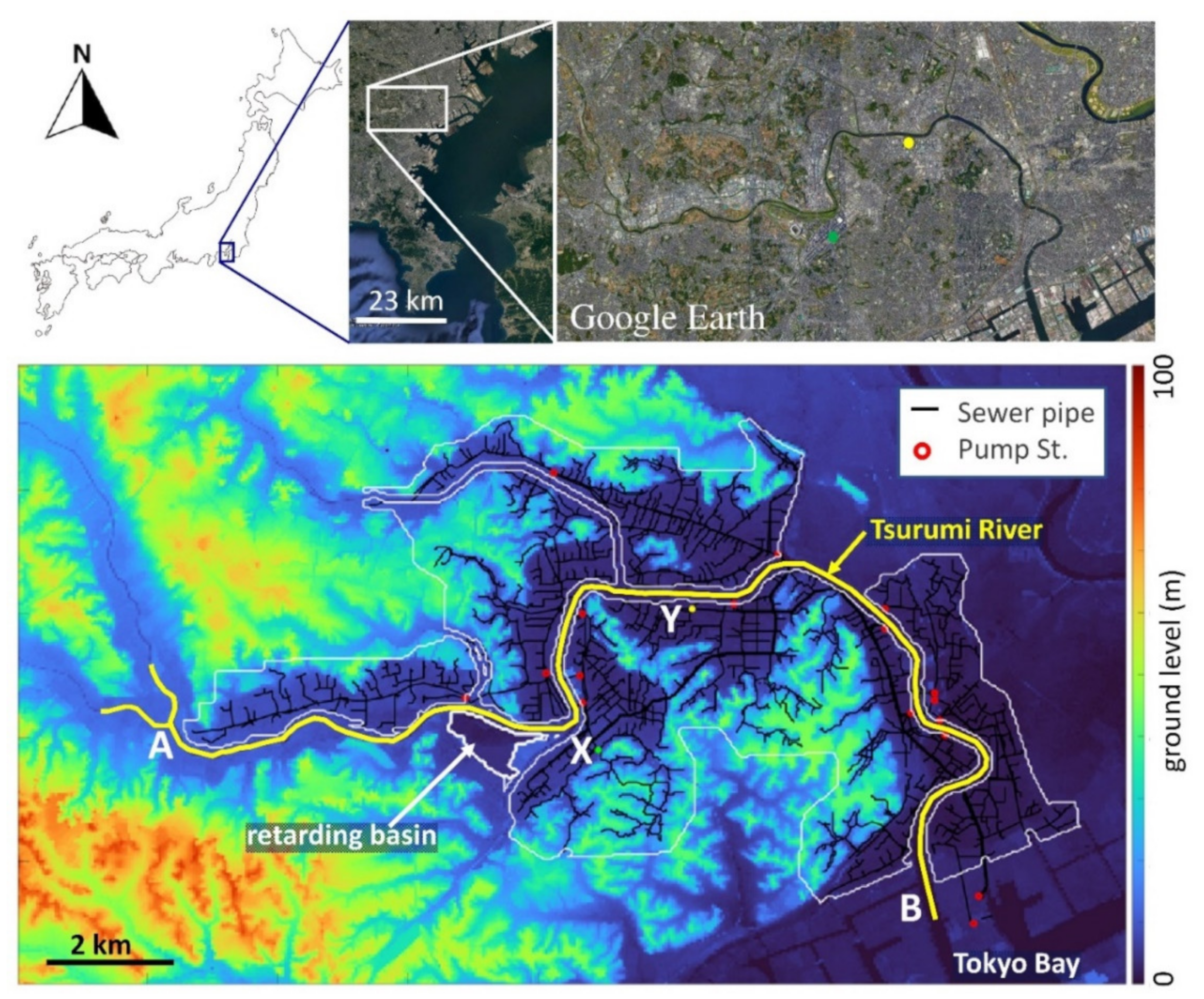
Figure 2 shows the location, topography, and trunk sewer network of the case study site, the Tsurumi River basin in Kanagawa Prefecture, Japan. In the figure, black lines indicate the trunk sewer networks with a diameter greater than 600 mm, the yellow line indicates the Tsurumi River, and red circles indicate the locations of the pumping station, at which the water is discharged from the sewer to the Tsurumi River. The Tsurumi River is also connected with the multi-purpose retarding basin with a total capacity of 3.9 million m3 bounded on the river side by an overflow-type levee. The area surrounded by a thin white line indicates each sub-catchment in which 2DG is computed. The points with X and Y indicate the locations of the Shin-Yokohama and Tarumachi manholes, respectively, at which the water levels are recorded. The capital characters A and B along the Tsurumi River indicate the locations of the upstream and downstream boundaries of 1DR, respectively. At the upstream boundary, time-varying discharge is determined by the measured water level and the H-Q curve at A. The downstream boundary condition is determined by the tide water level at the Tsurumi River mouth. In this case study site, the trunk sewer network pipelines have a total length of 336.7 km, and 8820 manholes connect these pipelines. Grid sizes of this case study were set to 200 m for 1DR and 40 m for 2DR and 1DS, respectively.
For the case study, we applied the heavy rainfall event induced by Typhoon Hagibis, which made landfall around Tokyo, Japan, on 12 October 2019. The spatiotemporal variation of the rainfall data was obtained from XRAIN with temporal and spatial resolution of 1 min and 250 m. In the model computation, linear interpolation was applied to specify the rainfall intensity at each grid and each time step.

2.3. Sensitivity Analysis

In this study, we apply PSO for auto-tuning of Manning’s roughness and the coefficient, α, for IWGDS shown in Equation (2). To capture the overall influence of these parameters, we first conducted the sensitivity analysis for these parameters. Table 1 lists the settings of these parameters in different cases. In the table, n 1 D R and n 1 D S indicate Manning roughness in the 1D River model (1DR) and 1D sewer network model (1DS), respectively. In case 0, the values of these parameters were obtained from the ones presented by Wu et al. [34]. As seen in the table, cases from A1 to A5 are for the sensitivity analysis of Manning roughness, whereas cases from B1 to B4 are for the coefficient, α, used in IWDGS.

2.4. Setup of PSO for Auto-Tuning of the Urban Flood Model

This section describes the setup of PSO for auto-tuning of the urban flood model. PSO was first introduced by Kennedy and Eberhart [36] and is one of the heuristic optimization algorithms that can solve large and complex NP-hard problems. The algorithm optimizes a problem by letting a large number of particles, called swarms, move around a given searching field. The location of each swarm in the searching field determines a candidate set of fitting parameters, and each swarm moves around to find the optimum location.
Figure 3 shows the flow chart of PSO developed in this study. In the figure, i identifies each swarm, and k is the number of iteration steps. Before iterative computations of swarms, the PSO system needs to determine: the number of swarms, M; and three weight parameters for the movement of swarms. Next, the initial locations of i-th swarms, X i , with i = 1, 2, … M, are randomly determined. Here, X i is a vector with N-dimensions. The vector component of each dimension determines the value of tuning parameters for the urban flood model. In each iteration step, each swarm is evaluated by an objective function.
The objective function for evaluation of each swarm is based on the Nash–Sutcliffe model efficiency coefficient, called NSE hereafter, determined by
NSE = 1 t = 1 T η o t η m t 2 t = 1 T η o t η ¯ o 2
where η o t is the observed water level at time, t, η m t is the computed water level at time, t, by the urban flood model, and η ¯ o is the observed mean water level over the period, T. The maximum value of NSE is unity when η m t and η o t perfectly match each other. On the other hand, the value of NSE decreases if the difference between η m t and η o t increases. In the present PSO, NSE is computed for each set of fitting parameters of each swarm, and the objective function is determined by F x , i = 1 NSE . Optimization of the swarm locations is thus conducted to minimize the objective function of each swarm.
If the computed objective function of i-th swarm at the present location, X i , is better than the best value of the same swarm in the past iterations, the personal best location of the i-th swarm, X P B , i , is replaced by X i . If the computed value of the objective function also exceeds the best of all the swarms in all the past iterations, then the global best location of all swarms in all the past iteration steps, X G B , is also renewed by X i . After updating X P B , i and X G B , the location of i-th swarm in the next iteration step, k + 1, is determined by:
X i k + 1 = X i k + V i k + 1
with
V i k + 1 = w V i k + c 1 r 1 X P B , i X i k + c 2 r 2 X G B X i k
where superscripts indicate the iteration steps, V i is a velocity vector of i-th swarm over an iteration step, w is inertia weight, c 1 and c 2 are weight parameters of relative influence of the personal and global best, respectively, and r 1 and r 2 are uniform random numbers between 0 and 1. The dimensions of the velocity vector should therefore be N, the dimension of X i . As seen in these equations, the velocity vector of the swarm is determined as a sum of weighted components of: (i) velocity vector of the swarm in the previous iteration step; and components proportional to the distance from X i to (ii) X P B , i and (iii) X G B , respectively. The relative importance of these components is determined by w , c 1 and c 2 . Following the existing studies, we set the values of these weighting parameters as w = 0.5, c 1 = 0.8 and c 2 = 0.9 . Although it is not shown in this paper, the performance of the present PSO applied to the urban flood model was tested with different values of these weighting parameters, and it was confirmed that aforementioned values yielded a good performance.

2.5. Application of PSO to the Case Study Site

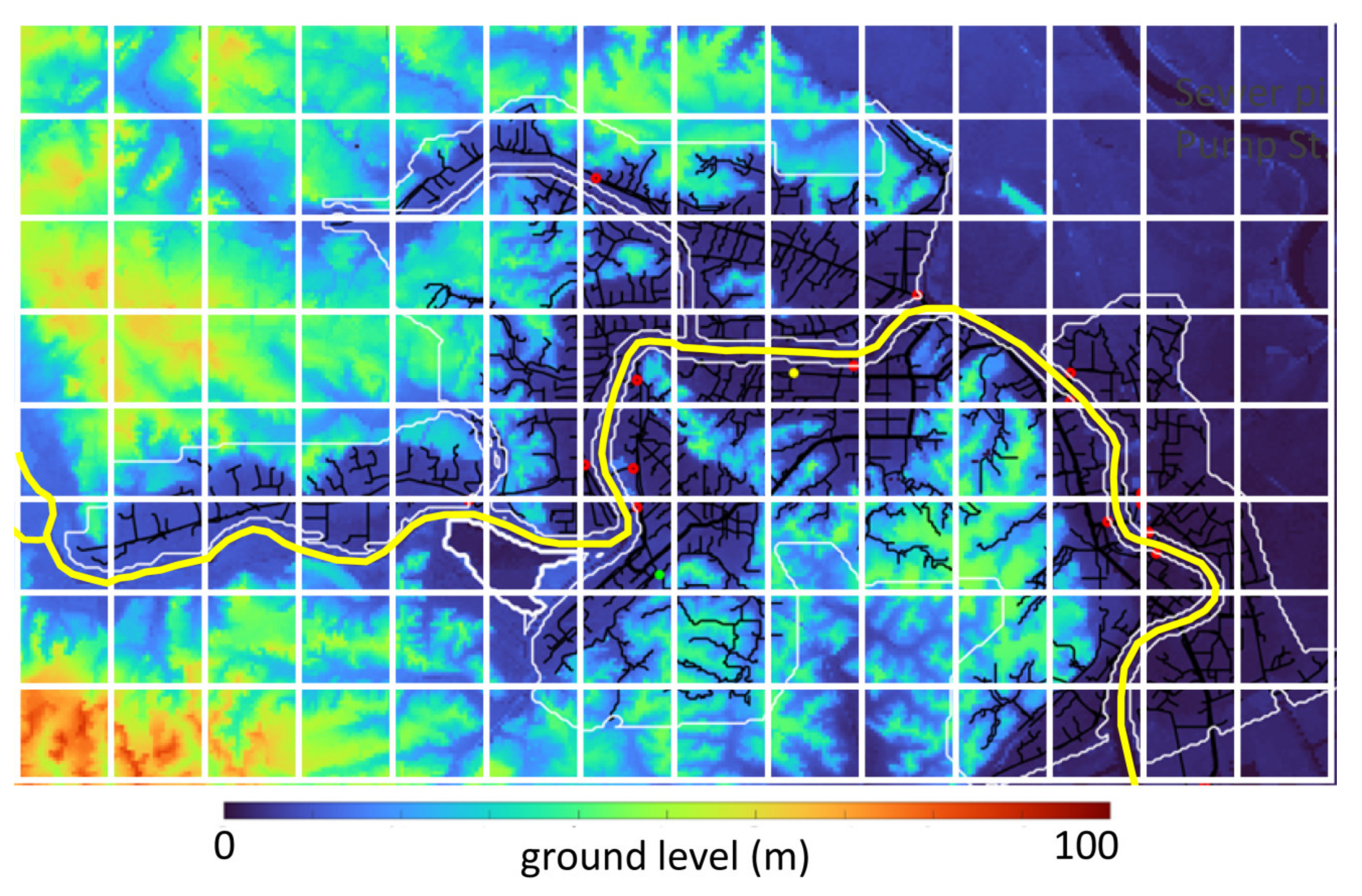
This section describes how the present PSO-based auto-tuning system of the urban flood model was applied to the case study site. The result of the sensitivity analysis described in Section 3.1 and Section 3.2 showed that the water level in the sewer system predicted by the urban flood model was moderately sensitive to the roughness of the sewer pipeline, and it was mildly dependent on the coefficient, α, of IWDGS. Since the optimum values of these parameters may vary at different locations, we split the computation domain evenly in east–west and north–south directions and find their optimum values in each section. Figure 4 shows an example of sections. In Figure 4, the number of sections in east–west direction, N x , is 14 while the number of sections in north–south direction, N y , is 8.
For the first trial, N x and N y were set to 20 and 10 for Manning roughness in the pipeline and 7 and 4 for the coefficient, α. While the number of segmented sections becomes 200 and 28, respectively, some of these sections contain no sewer pipelines or not connected to the sewer network. After removal of these sections, the total number of sections used in this first trial became 112 and 20. In this first trial case, the number of dimensions of vectors, X i , in Equation (4) becomes 132, the sum of these sections that contain sewer pipelines. Initial values of Manning’s roughness, n, and coefficient, α, of each swarm were randomly determined so that selected quantities are uniformly distributed within the range of 0.01 (s/m1⁄3) < n < 0.03 (s/m1⁄3) and 4 (m) < α < 6 (m), respectively. In this study, the validity of the present PSO is tested for different combinations of N x and N y . Overall predictive skills of the auto-tuned urban flood model were then evaluated by NSE, Kling–Gupta efficiency (KGE), Root Mean Square Error (RMSE), and normalized RMSE (NRMSE).
While the larger number of tuning parameters may improve NSE, it may lead to overfitting of the model and may deteriorate the model applicability to different rainfall events. To investigate the appropriate number of fitting parameters, this study also compared AIC (Akaike’s Information Criterion) [37] of three cases in which different numbers of ( N x , N y ) were applied. Since the number of observed sampling data is limited, this study applied AICc, modified AIC for a relatively small number of samples [38].
In three different cases, the numbers of ( N x , N y ) for segmentation of Manning’s roughness in the sewer pipelines were set for (10, 10), (20, 10), and (10, 20), respectively. In these three cases, the number of segmented roughness parameters became 66, 112, and 116, respectively. In all cases, the number of segmentations of coefficient, α, was fixed for ( N x , N y ) = (14, 8) since it was confirmed that the model was not sensitive to this coefficient.

3. Results and Discussions

3.1. Model Sensitivity to Manning’s Roughness

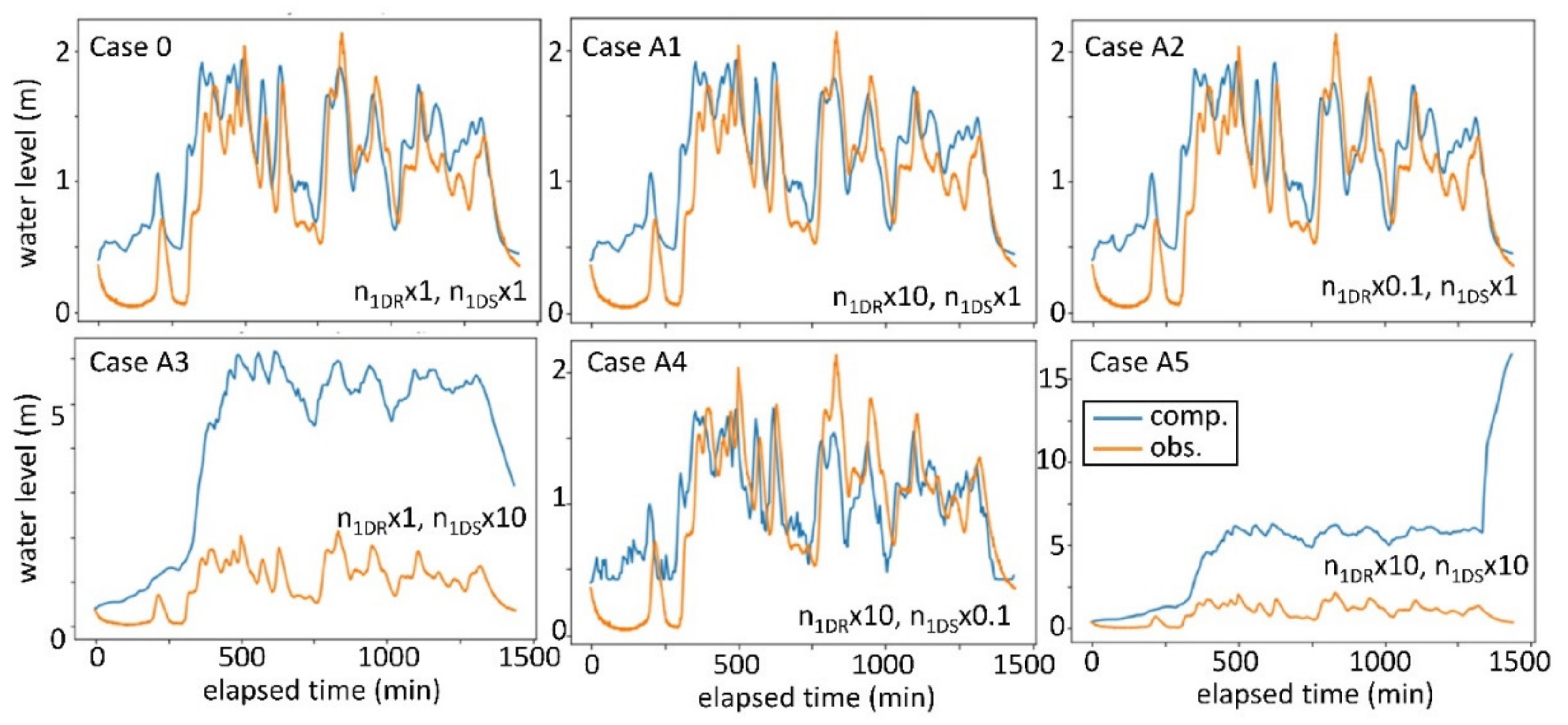
Figure 5 compares the computed and measured time series of the water level at the Shin-Yokohama manhole, indicated by X in Figure 2. Little difference in the result of cases 0, A2 and A5 indicates that Manning roughness along the riverbed has little influence on the computed water levels at the Shin-Yokohama manhole. Since the river and the sewer networks are connected by pumping stations and the pumping rate is not dependent on the river water level, the computed water level in the sewer pipeline is not affected by the river water level, i.e., the Manning roughness along the river. On the other hand, a significant difference was observed between the results of cases 0 and A1, where case A1 applied a 10 times larger Manning roughness along the sewer pipeline. A relatively minor difference was found between cases A2 and A3, where case A3 applied a 10 times smaller roughness along the pipeline. These results indicate that the flow rate along the sewer pipeline is dominantly determined by roughness if the roughness is relatively large, while the flow rate in the sewer pipeline is dominantly determined by other factors, such as pumping rate, if the roughness is sufficiently small. Based on these results, the present auto-tuning system focuses on the tuning of Manning roughness along the sewer network, but not along the riverbed.

3.2. Model Sensitivity to the Coefficient, α

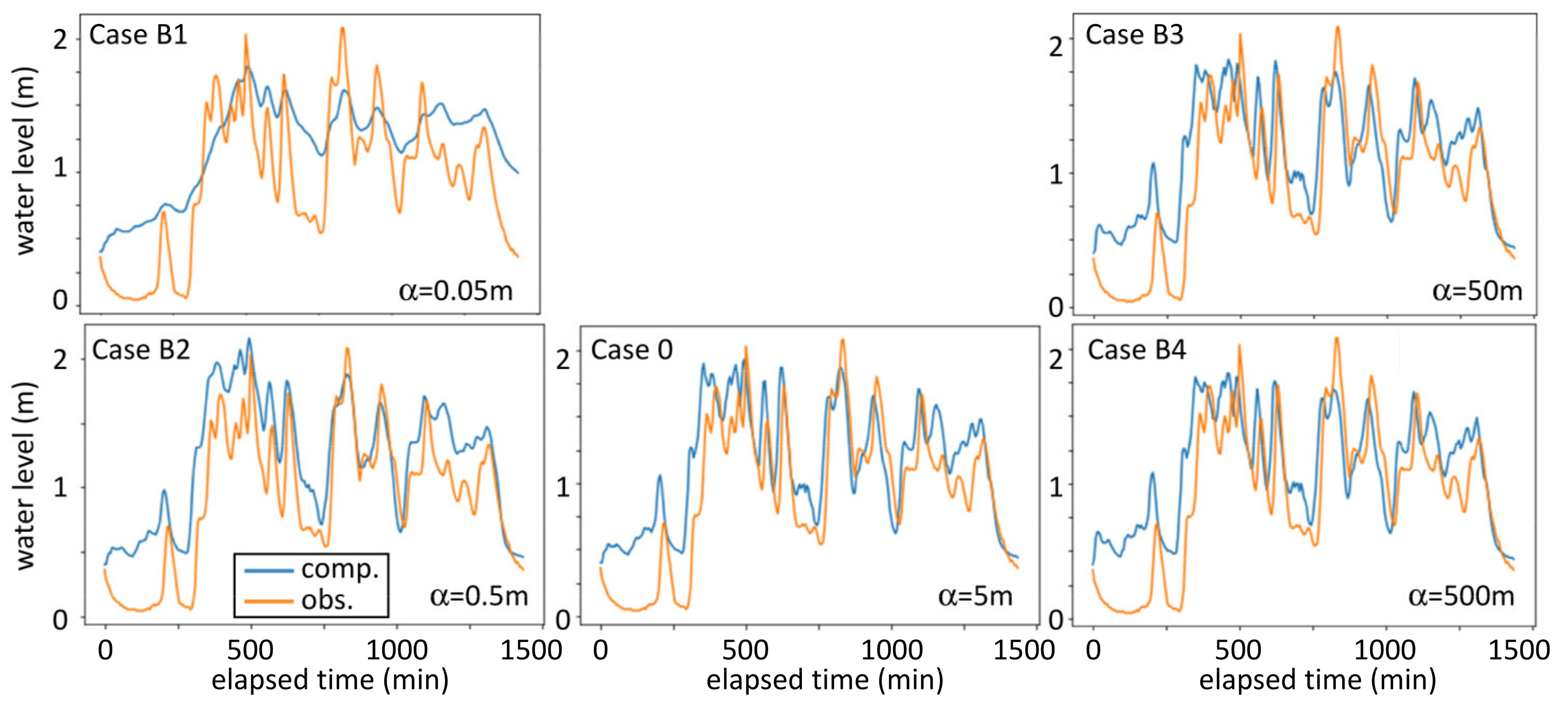
Figure 6 also compares the time-series of computed and measured water level at Shin-Yokohama manhole for cases, 0, B1, B2, B3 and B4, in which different values of the coefficient, α, in Equation (2) were applied. Based on the comparisons of these cases, it can be concluded that the computed water levels are sensitive to α if the value of α is lower than 5 m. The water discharge from the ground to the sewer should be increased by increasing the value of α, but the maximum amount should be limited by the total volume of water remaining on the ground. In this sense, auto-tuning of α should be performed against the heavy rainfall event so that the clear influence of the value of α can be detected in the model computations. The heavy rainfall event induced by Typhoon Hagibis in 2019 is therefore suitable for application of the present auto-tuning system for estimation of the value of α. It is also interesting to note that the computed water level tends to be higher in case B2 with α = 0.5 m than the one in case 0 with α = 0.5 m after the elapsed time later than 300 min. The smaller α yields lower discharge to the sewer, but this relatively lower discharge in case B2 lasts longer than in case 0. This lower but longer discharge could delay and elevate the peak water level inside the sewer pipeline. The complex response of the sewer water level against those parameters may also support the merit of the present auto-tuning system.

3.3. Application of the Present PSO-Based Auto-Tuning System

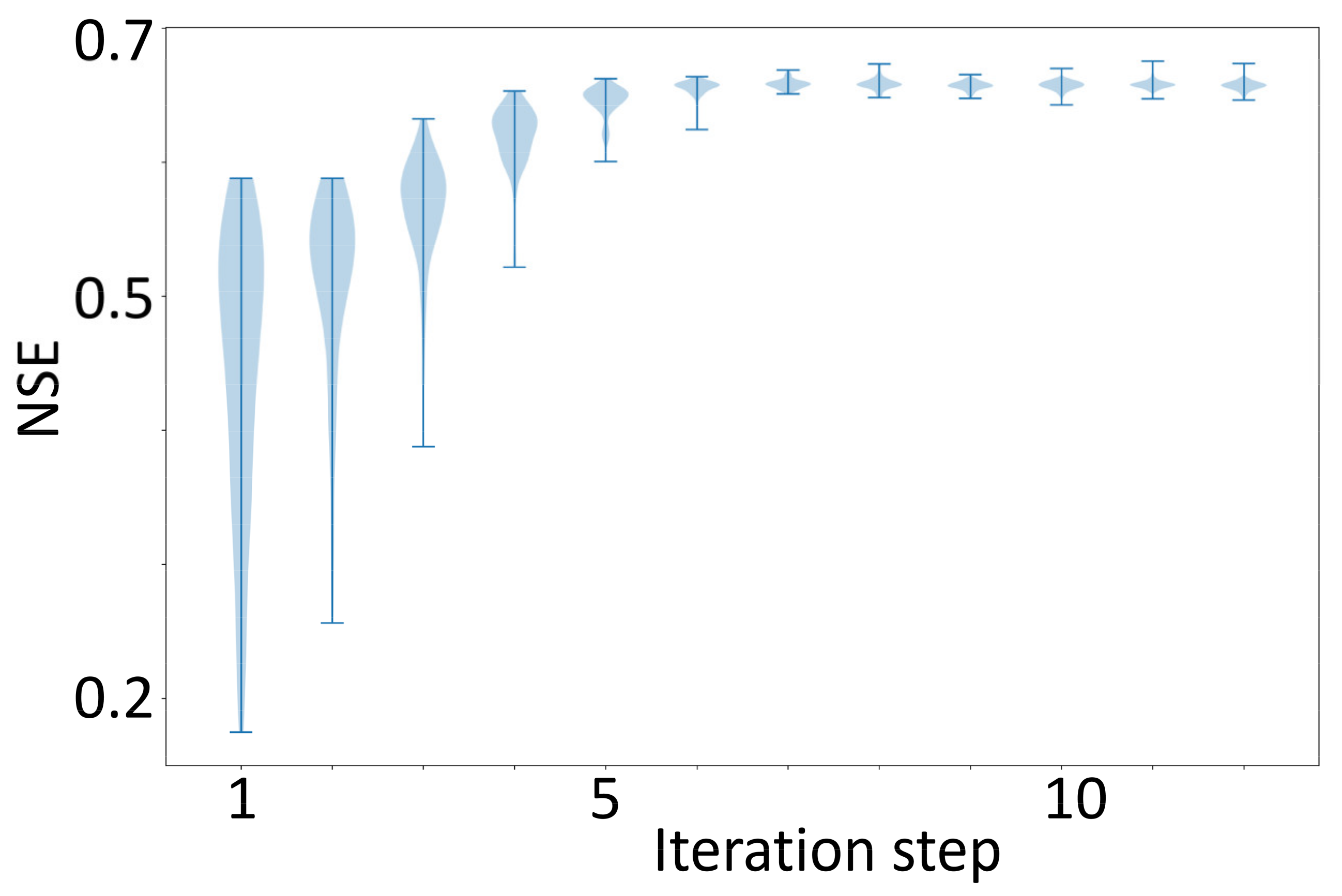
Figure 7 shows the violin plot of computed NSE at each iteration step, i when ( N x , N y ) = (20, 10) for Manning’s roughness and ( N x , N y ) = (14, 8) for coefficient α. Here, the number of swarms is 100 and the iteration for the travel of each swarm was conducted 12 times. In all iterations, the highest NSE, 0.69, was obtained in the 11th iteration step.
Table 2 compares NSE, KGE, RMSE and NRMSE of computed results with and without auto-tuning. Here, the results of case 0 were used for the case without auto-tuning. It should be noted that case 0 is based on the spatially uniform parameter values used by Wu et al. [34], who manually calibrated the parameter values. The value of KSE ranges from negative infinity to unity and approaches unity for a perfect match between the computed results and measurements. As seen in the table, the predictive performance of the urban flood model is clearly improved by the present auto-tuning system.
For different sets of ( N x , N y ), i.e., ( N x , N y ) = (10, 10), (20, 10), and (10, 20), the computed AICc were 0.296, 0.317, and 1.668, respectively. Clearly, a higher AICc was obtained when ( N x , N y ) = (10, 20), indicating that N y = 20 is too large to avoid the overfitting. Among these three cases, the case with ( N x , N y ) = (10, 10), the minimum number of parameters, yielded the lowest AICc. The following discussions therefore focus on this case.
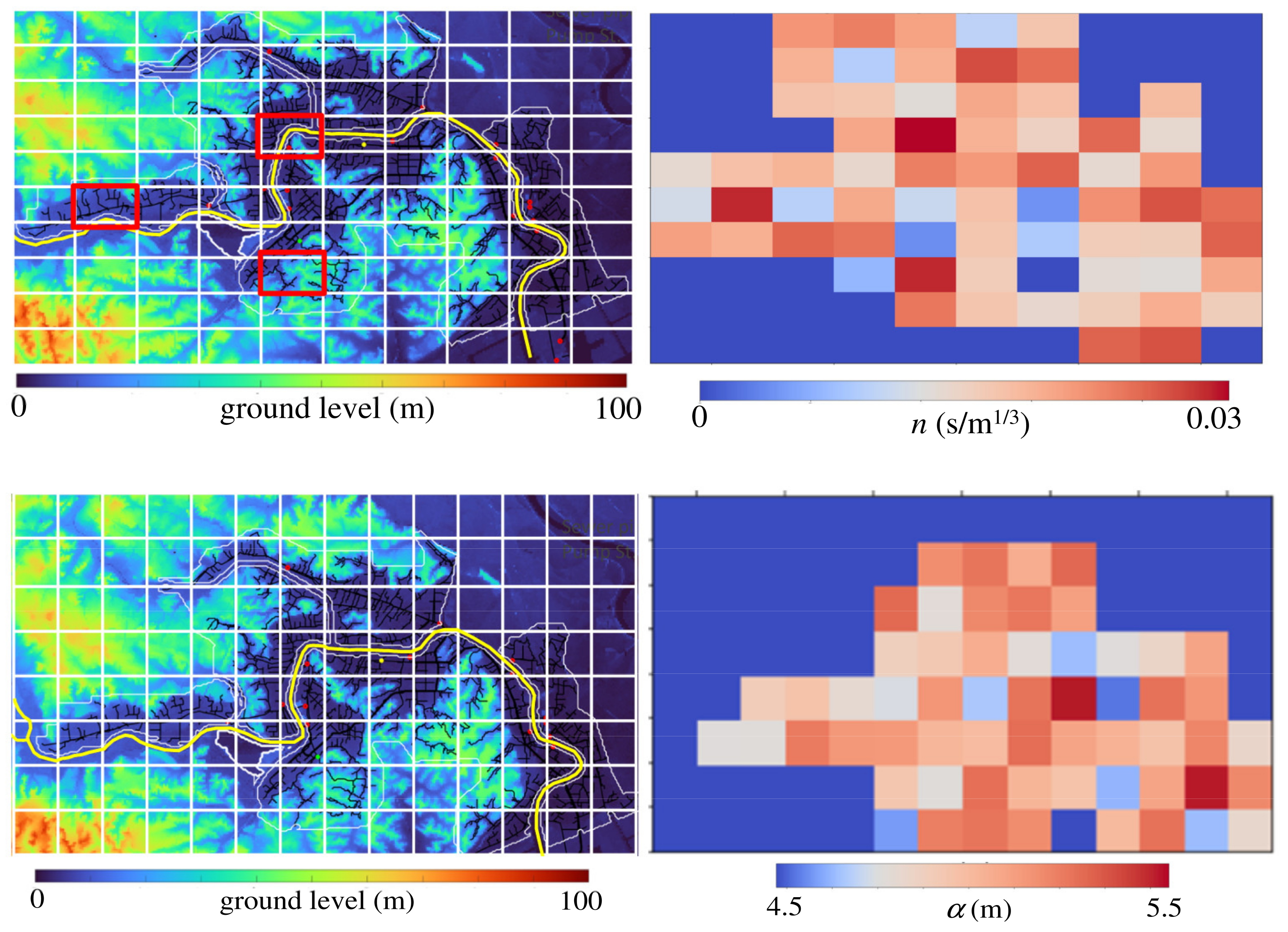
Figure 8 shows the spatial distribution of auto-tuned Manning’s roughness, n, and coefficient, α, for the case of ( N x , N y ) = (10, 10) for Manning’s roughness and ( N x , N y ) = (14, 8) for coefficient α, respectively. In the figure, the square segment colored in blue is the segment in which there are no sewer pipelines or no connections to the sewer through IWDGS. While obtained α are concentrated within a relatively narrow range around the value, α = 5 (m), used by the previous study (Wu et al. [34]), the value of Manning’s roughness showed certain variation. It is interesting to note that relatively high roughness is obtained in the upstream branch of the sewer pipelines indicated by red squares. These results highlight the importance of setting the spatial variation of Manning’s roughness for more accurate predictions of the flow in sewer pipelines, and thus support the effectiveness of the present PSO-based auto-tuning system.

4. Conclusions

This paper studied the auto-tuning system of the complex urban flood model based on PSO, which has an advantage in computationally efficient optimization of complex systems. Sensitivity analysis was first conducted for roughness and coefficient α of the present urban flood model. It was found that the computed water level inside the sewer pipeline was moderately sensitive to the roughness of the sewer pipeline, while it was weakly sensitive the coefficient α of the discharge from the land to the sewer and was not sensitive to the river bed roughness.
A PSO-based auto-tuning system was then constructed for auto-tuning of the spatial distribution of the roughness of sewer pipelines and coefficient α. Clear improvements of the accuracy of computed water level inside the pipeline were achieved by the developed auto-tuning system. Predictive performance of the model computation was evaluated by NSE, KGE, RMSE and NRMSE, and it was found that NSE of computed results of each swarm particle converges quickly within several iterations. Besides these indicators, this study computed modified Akaike Information Criteria, AICc, for each case with a different number of spatial segments, in each of which Manning’s roughness and coefficient α are, respectively, optimized. In this case study, a relatively lower number of segments yielded the smaller AICc, indicating that the present urban flood model requires relatively coarse spatial resolution of the variation of roughness and coefficient to obtain reasonable predictive skills of the time-varying water level inside the sewer pipeline. While the proposed PSO-based auto-tuning system for the urban flood model showed a reasonable potential, more analysis with different cases and different optimization algorithms should be added for further understanding, evaluations, and improvements of the system.

Author Contributions

Conceptualization, Y.T. and L.J.; methodology, L.J. and Y.T.; original model, L.W. and Y.T.; validation, L.J., Y.T. and L.W.; analysis and investigation, L.J.; data curation, L.W.; writing—original draft preparation, Y.T. and L.J.; writing—review and editing, Y.T. and L.W.; visualization, L.J., Y.T. and L.W.; supervision, Y.T.; funding acquisition, Y.T. All authors have read and agreed to the published version of the manuscript.

Funding

This study was conducted as a research activity of “Enhancement of National Resilience against Natural Disasters”, Cross-ministerial Strategic Innovation Promotion Program (SIP), under the supervision of NIED, Japan. The program was supported by the Council for Science, Technology, and Innovation (CSTI), Japan.

Institutional Review Board Statement

Not applicable.

Informed Consent Statement

Not applicable.

Data Availability Statement

The data of topography and sewer pipelines were provided by Yokohama City. The measured water level data were obtained by authors, and are available upon reasonable request.

Conflicts of Interest

The authors declare no conflict of interest.

References

  1. O’Donnell, E.C.; Thorne, C.R. Drivers of future urban flood risk. Philos. Trans. R. Soc. A 2020, 378, 23. [Google Scholar] [CrossRef] [PubMed]
  2. Ashley, R.; Garvin, S.; Pasche, E.; Vassilopoulos, A.; Zevenbergen, C. Advances in Urban Flood Management; CRC Press: Boca Raton, FL, USA, 2007. [Google Scholar] [CrossRef]
  3. Kundzewicz, Z.W.; Kanae, S.; Seneviratne, S.I.; Handmer, J.; Nicholls, N.; Peduzzi, P.; Mechler, R.; Bouwer, L.M.; Arnell, N.; Mach, K.; et al. Flood risk and climate change: Global and regional perspectives. Hydrol. Sci. J. 2014, 59, 1–28. [Google Scholar] [CrossRef]
  4. Miller, J.D.; Hutchins, M. The impacts of urbanisation and climate change on urban flooding and urban water quality: A review of the evidence concerning the United Kingdom. J. Hydrol.-Reg. Stud. 2017, 12, 345–362. [Google Scholar] [CrossRef]
  5. Shaw, R.; Surjan, A.; Parvin, G.A. Urban Disasters and Resilience in Asia; Butterworth-Heinemann: Oxford, UK, 2016. [Google Scholar]
  6. Adnan, M.S.G.; Abdullah, A.M.; Dewan, A.; Hall, J.W. The effects of changing land use and flood hazard on poverty in coastal Bangladesh. Land Use Policy 2020, 99, 104868. [Google Scholar] [CrossRef]
  7. Yin, J.; Yu, D.P.; Yin, Z.; Liu, M.; He, Q. Evaluating the impact and risk of pluvial flash flood on intra-urban road network: A case study in the city center of Shanghai, China. J. Hydrol. 2016, 537, 138–145. [Google Scholar] [CrossRef]
  8. Huong, H.T.L.; Pathirana, A. Urbanization and climate change impacts on future urban flooding in Can Tho city, Vietnam. Hydrol. Earth Syst. Sci. 2013, 17, 379–394. [Google Scholar] [CrossRef]
  9. Hallegatte, S.; Green, C.; Nicholls, R.J.; Corfee-Morlot, J. Future flood losses in major coastal cities. Nat. Clim. Chang. 2013, 3, 802–806. [Google Scholar] [CrossRef]
  10. Hammond, M.J.; Chen, A.S.; Djordjevic, S.; Butler, D.; Mark, O. Urban flood impact assessment: A state-of-the-art review. Urban Water J. 2015, 12, 14–29. [Google Scholar] [CrossRef]
  11. Henonin, J.; Russo, B.; Mark, O.; Gourbesville, P. Real-time urban flood forecasting and modelling–a state of the art. J. Hydroinform. 2013, 15, 717–736. [Google Scholar] [CrossRef]
  12. DHI. MIKE-Flood User Manual. Available online: https://manuals.mikepoweredbydhi.help/2021/Water_Resources/MIKE_FLOOD_UserManual.pdf (accessed on 29 July 2022).
  13. Xpswmm Reference Manual. Available online: https://dokumen.tips/documents/xpswmm-reference-manual.html?page=37 (accessed on 29 July 2022).
  14. Innovyze. InfoWorks ICM Help Documentation. Available online: https://help.innovyze.com/display/infoworksicm/Table+of+Contents (accessed on 29 July 2022).
  15. Qi, W.C.; Ma, C.; Xu, H.S.; Chen, Z.F.; Zhao, K.; Han, H. A review on applications of urban flood models in flood mitigation strategies. Nat. Hazards 2021, 108, 31–62. [Google Scholar] [CrossRef]
  16. Piadeh, F.; Behzadian, K.; Alani, A.M. A critical review of real-time modelling of flood forecasting in urban drainage systems. J. Hydrol. 2022, 607, 16. [Google Scholar] [CrossRef]
  17. Ravazzani, G.; Amengual, A.; Ceppi, A.; Homar, V.; Romero, R.; Lombardi, G.; Mancini, M. Potentialities of ensemble strategies for flood forecasting over the Milano urban area. J. Hydrol. 2016, 539, 237–253. [Google Scholar] [CrossRef]
  18. Shrestha, A.; Mascaro, G.; Garcia, M. Effects of stormwater infrastructure data completeness and model resolution on urban flood modeling. J. Hydrol. 2022, 607, 18. [Google Scholar] [CrossRef]
  19. Paquier, A.; Bazin, P.H. Estimating uncertainties for urban floods modelling. Houille Blanche-Revue Internationale De L Eau. La Houille Blanche 2014, 6, 13–18. [Google Scholar] [CrossRef]
  20. Yu, D.P.; Coulthard, T.J. Evaluating the importance of catchment hydrological parameters for urban surface water flood modelling using a simple hydro-inundation model. J. Hydrol. 2015, 524, 385–400. [Google Scholar] [CrossRef]
  21. Bellos, V.; Kourtis, I.M.; Moreno-Rodenas, A.; Tsihrintzis, V.A. Quantifying Roughness Coefficient Uncertainty in Urban Flooding Simulations through a Simplified Methodology. Water 2017, 9, 944. [Google Scholar] [CrossRef]
  22. Ehteram, M.; Othman, F.B.; Yaseen, Z.M.; Afan, H.A.; Allawi, M.F.; Malek, M.B.A.; Ahmed, A.N.; Shahid, S.; Singh, V.P.; El-Shafie, A. Improving the Muskingum Flood Routing Method Using a Hybrid of Particle Swarm Optimization and Bat Algorithm. Water 2018, 10, 807. [Google Scholar] [CrossRef]
  23. He, Y.Y.; Wan, J.H. Flood hazard assessment based on fuzzy clustering iterative model and chaotic particle swarm optimization. J. Ambient. Intell. Humaniz. Comput. 2021, 12, 933–942. [Google Scholar] [CrossRef]
  24. He, Y.Y.; Xu, Q.F.; Yang, S.L.; Liao, L. Reservoir flood control operation based on chaotic particle swarm optimization algorithm. Appl. Math. Model. 2014, 38, 4480–4492. [Google Scholar] [CrossRef]
  25. Peng, Y.; Ye, S.G.; Zhou, H.C.; Kang, H.G.; IEEE. Model of Flood Control Operation of Reservoir Based on Particle Swarm Optimization Algorithm and Its Application. Proc. Int. Conf. Comput. Sci. Netw. Tech. 2011, 1, 368–371. [Google Scholar]
  26. Storn, R.; Price, K. Differential Evolution—A Simple and Efficient Heuristic for global Optimization over Continuous Spaces. J. Glob. Optim. 1997, 11, 341–359. [Google Scholar] [CrossRef]
  27. Yazdani, M.; Jolai, F. Lion Optimization Algorith, (LOA): A nature-inspired metaheuristic algorithm. J. Comput. Des. Eng. 2016, 3, 24–36. [Google Scholar] [CrossRef]
  28. Fathollahi-Fard, A.M.; Hajiaghaei-Keshteli, M.; Tavakkoli-Moghaddam, R. Red deer algorithm (RDA): A new nature-inspired meta-heuristic. Soft Comput. 2020, 24, 14637–14665. [Google Scholar] [CrossRef]
  29. Kuok, K.K.; Harun, S.; Shamsuddin, S.M. Particle swarm optimization feedforward neural network for modeling runoff. Int. J. Envir. Sci. Tech. 2010, 7, 67–78. [Google Scholar] [CrossRef]
  30. Niu, W.J.; Feng, Z.K.; Cheng, C.T.; Zhou, J.Z. Forecasting Daily Runoff by Extreme Learning Machine Based on Quantum-Behaved Particle Swarm Optimization. J. Hydrol. Eng. 2018, 23, 04018002. [Google Scholar] [CrossRef]
  31. Romlay, M.R.M.; Rashid, M.M.; Toha, S.F. Development of Particle Swarm Optimization Based Rainfall-Runoff Prediction Model for Pahang River, Pekan. In Proceedings of the 2016 International Conference on Computer and Communication Engineering, Kuala Lumpur, Malaysia, 26–27 July 2016; pp. 306–310. [Google Scholar]
  32. Taormina, R.; Chau, K.W. Data-driven input variable selection for rainfall-runoff modeling using binary-coded particle swarm optimization and Extreme Learning Machines. J. Hydrol. 2015, 529, 1617–1632. [Google Scholar] [CrossRef]
  33. Tada, T. Parameter Optimization of Hydrological Model Using the PSO Algorithm. J. Jpn. Soci. Hydro. Water Res. 2007, 20, 450–461. [Google Scholar] [CrossRef]
  34. Wu, L.H.; Tajima, Y.; Sanuki, H.; Shibuo, Y.; Furumai, H. A novel approach for determining integrated water discharge from the ground surface to trunk sewer networks for fast prediction of urban floods. J. Flood Risk Manag. 2022, 15, 17. [Google Scholar] [CrossRef]
  35. Chaudhry, M.H. Applied Hydraulic Transients; Springer: New York, NY, USA, 1979. [Google Scholar]
  36. Kennedy, J.; Eberhart, R. Particle swarm optimization. Proc. Int. Conf. Neural Netw. 1995, 1, 1942–1948. [Google Scholar]
  37. Akaike, H. A new look at the statistical model identification. IEEE Trans. Autom. Control. 1974, 19, 716–723. [Google Scholar] [CrossRef]
  38. Cavanaugh, J.E.; Shumway, R.H. A bootstrap variant of AIC for state-space model selection. Stat. Sin. 1997, 7, 473–496. [Google Scholar]
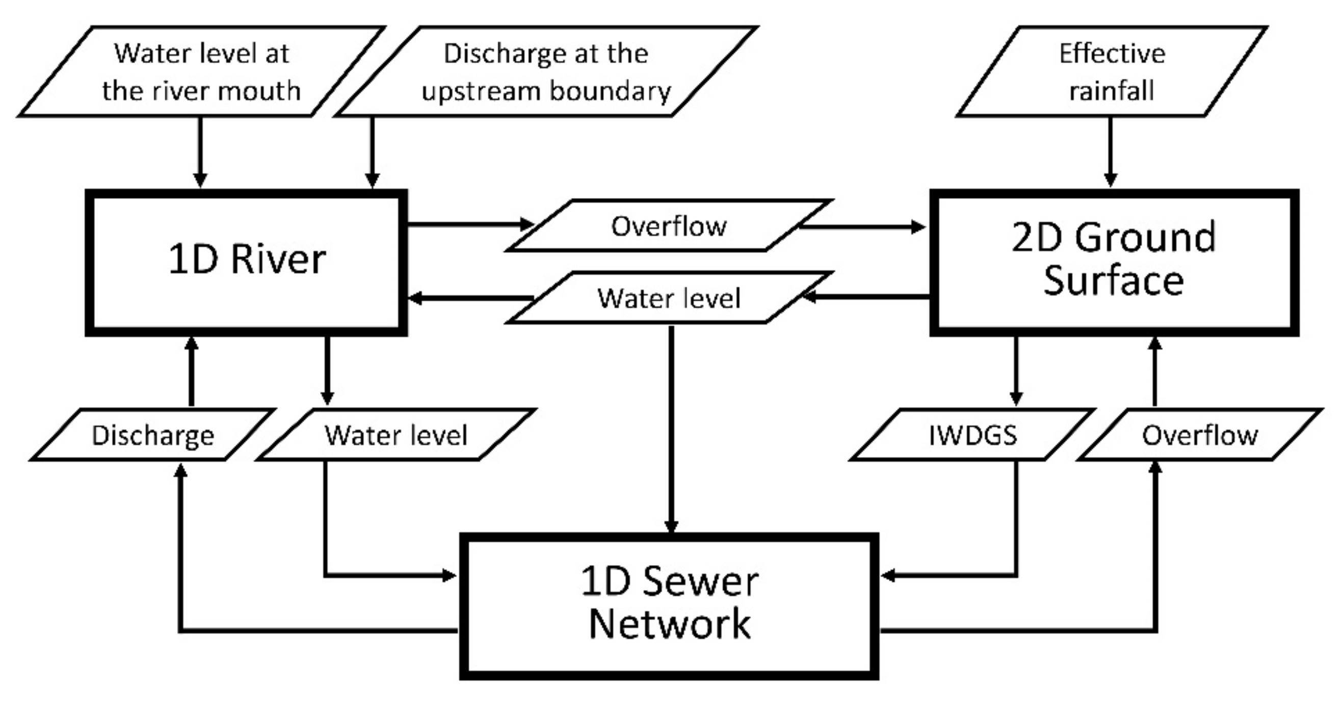
Figure 1. Schematic chart of the urban flood model (Wu et al., 2022) [34].
Water 14 02819 g001
Figure 2. Locations and computational domain of the case study site, the Tsurumi River basin, Japan.
Water 14 02819 g002
Figure 3. Flow chart of the calculation procedure in the PSO algorithm.
Water 14 02819 g003
Figure 4. An example of evenly segmented sections ( N x = 14 and N y = 8 ).
Water 14 02819 g004
Figure 5. Comparisons of the time-varying water level at the Shin-Yokohama manhole in cases 0, A1, A2, A3, A4 and A5. In the figure, n1DR and n1DS are the roughness of the river bed and the pipeline for case 0, respectively.
Water 14 02819 g005
Figure 6. Comparisons of the time-varying water level at the Shin-Yokohama manhole in cases 0, B1, B2, B3, and B4.
Water 14 02819 g006
Figure 7. Violin plot of NSE of each swarm at different iteration step, i.
Water 14 02819 g007
Figure 8. Spatial distribution of the tuned Manning’s roughness (top) and the coefficient, α (bottom).
Water 14 02819 g008
Table 1. Parameter settings of the sensitivity analysis of the urban flood model.
Case n 1 D R ( sm 1 / 3 ) n 1 D S ( sm 1 / 3 ) α (m)
00.0250.0135
A10.250.0135
A20.00250.0135
A30.0250.135
A40.250.00135
A50.250.135
B10.0250.0130.05
B20.0250.0130.5
B30.0250.01350
B40.0250.013500
Table 2. Comparisons of performance metrics, NSE, KGE, RMSE and NRMSE, of the computed results before and after the auto-tuning.
CaseNSEKGERMSE (m)NRMSE
case 00.55−0.700.360.23
after tuning0.690.650.290.19
Publisher’s Note: MDPI stays neutral with regard to jurisdictional claims in published maps and institutional affiliations.