Article

The Impact of Rainfall on Soil Moisture Variability in Four Homogeneous Rainfall Zones of India during Strong, Weak, and Normal Indian Summer Monsoons

1
Center for Ocean-Atmospheric Prediction Studies, The Florida State University, Tallahassee, FL 32306, USA
2
Department of Earth, Ocean, Atmospheric Science, The Florida State University, Tallahassee, FL 32306, USA
3
Andhra Pradesh State Disaster Management Authority, Kunchanapalli 522501, Andhra Pradesh, India
*
Author to whom correspondence should be addressed.
Water 2022, 14(18), 2788; https://doi.org/10.3390/w14182788
Submission received: 26 July 2022 / Revised: 2 September 2022 / Accepted: 5 September 2022 / Published: 8 September 2022
(This article belongs to the Section Soil and Water)

Abstract

:
This observational study mainly examines the impact of rainfall on Indian soil moisture (SM) variability in four homogeneous rainfall zones (i.e., central India (CI), northwest India (NWI), south peninsula India (SPIN), and northeast India (NEI)) as defined by India Meteorological Department (IMD) during strong, weak, and normal Indian summer monsoons (ISMs), which are determined regionally for each homogeneous rainfall zone separately. This study uses the daily gridded (0.25° × 0.25°) rainfall data set provided by IMD and the daily gridded (0.25° × 0.25°) SM combined product version 06.1 from European Space Agency Climate Change Initiative (ESA CCI) over the period 1992–2020. Results reveal that monthly and seasonal mean SM in NWI, CI, and SPIN are overall higher during strong than during weak ISMs. The daily SM and its dependence on rainfall appear to be region-locked in space and phase-locked in time: Strong correlation and large response to rainfall generally occur in most parts of SPIN and NWI during June (June–July) of strong (weak) ISMs where SM values are relatively small; Weak correlation and small response generally occur in CI and NEI in July-September (August–September) of strong (weak) ISMs where SM values are relatively large. The phase-locked feature is associated with the features of ISMs. The region-locked feature is presumably associated with the local features, such as soil and vegetation types and/or environmental conditions. Both region-locked and phase-locked features cause regional distinct features in SM persistence.

1. Introduction

Soil moisture (SM) is essential for local agriculture, particularly for India which feeds the large population [1] and makes up a large fraction of the Indian economy [2]. India’s rain-fed agriculture is largely dependent on soil types and available SM. SM in India is generally controlled by Indian monsoon rainfall, evapotranspiration, and horizontal and downward transport of water provided by the water balance equation:
ΔSM = R − ET − TR
where ΔSM, R, ET, and TR represent changes in SM, rainfall, evapotranspiration, and horizontal and downward transport of water, respectively. Rainfall is the primary source of SM, TR can be source or sink, and ET is a sink according to the water balance equation. Approximately 16% of India’s geographic area is drought-prone, mostly arid, or semiarid [3] and SM variations in time and space are critically important for crop sustenance and subsequent crop yield, particularly during active and weak phases of ISM seasons (i.e., June through September). The wide-range shortage of SM (i.e., major drought events) in India is primarily caused by the large-scale negative rainfall anomalies [4].
However, the high spatial coverage and high temporal-spatial sampling rate of SM were not readily available until the advent of spaceborne measurements. Historical records of direct measurements of the dryness and wetness of the ground (e.g., SM content) are sparse in both time and space [5], which significantly limited our studies related to the variability of SM in time and space. Additionally, the cost of direct observations of SM is extremely high and they represent single-point observations alone in space. On the other hand, remote sensing techniques offer an alternative and economical way to estimate the SM over a large area. The retrievals from individual soil moisture platforms using remote sensing techniques are combined using statistical techniques to a reference land model, yielding a model-like soil moisture product [6]. For example, the European Space Agency Climate Change Initiative (ESA CCI) provides modeled estimated SM products by combining the retrievals to land a reference model: The “active product” (derived from scatterometers), the “passive product” (derived from radiometers), and the “combined product” (derived from the “active” and “passive” products) [7]. These products will allow us to study the variability of SM in space and time with far greater detail than would be possible with in situ observations. However, a relatively minor weakness is that the satellite observations apply to the time of a satellite overpass (or the average of these times), whereas the in situ system may apply to a specific time of day. The difference in measurement depth as well as the difference in timing between in situ and satellite observations could be responsible for considerable differences on a day-to-day comparison, but otherwise, does not adversely impact the use of satellite data. For example, Sathyanadh et al. [8] revealed good agreement in SM between in situ observations and ESA CCI SM product with respect to several statistical estimates, such as bias, unbiased root-mean-squared difference, and normalized standard deviations.
Several studies have focused on the Indian SM features as well as the association of SM with the Indian summer monsoon rainfall (ISMR). For example, Liu et al. [9] found a positive statistical correlation between SM and precipitation in India on seasonal and interannual timescales, but they did not explain what causes this relationship. Shrivastava et al. [10] examined the SM features in central India with ESA CCI SM product over the period 2002–2011 and showed that SM in central India is very well correlated with the observed gridded rainfall during dry spells of 10 ISM periods (i.e., June through September, or JJAS in short). Pangaluru et al. [11] examined SM variability in India and found a good relationship with precipitation based on monthly mean fields. Singh et al. [12] studied the monthly and seasonal variations of SM in India using Indian Remote Sensing satellite data, suggesting strong geographic monthly and seasonal variations.
Sathyanadh et al. [8], a study most relevant to the present study, examined the spatial and temporal characteristics of SM and its association with monsoon rainfall during a weak (2002) and a strong 2007 ISM using MERRA-land global reanalysis SM dataset and the IMD daily gridded rainfall data. They found that large intraseasonal variations of SM contribute to interannual variations of SM and SM variations on intraseasonal and interannual timescales follow the rainfall pattern. Moreover, they observed that the dominant modes (at timescales of 2–10 days, 20–30 days, and above) of SM are dependent on geographic location, monsoon duration, intraseasonal rainfall variations, and SM persistence. The present study differs from the recent three studies [8,10,12]; at least in three aspects: (1) This study examines the distinct dependence of SM on monsoon rainfall based on the rainfall strengths on regional scales during the period 1992–2020, which differs from the study by Sathyanadh et al. [8] which was based on a single weak (2002) and a single strong ISM (2007) only and also differs from the study by Shrivastava et al. [10] which was based on specified dry spells of ISM; (2) this study also examines the dependence of SM on rainfall using daily values and not on seasonal and interannual timescales as Singh et al. [12] did using monthly data, and further illustrates how the dependence changes for different strengths of ISMs, which has not yet been explored, and (3) this study is focused on the analysis of observed SM features and its dependence on rainfall on regional scales. Based on the coherent rainfall on regional scales, the IMD defined four so-called homogeneous regions: Northwest India (NWI), northeast India (NEI), central India (CI), and south peninsula India (SPIN), as shown in Figure 1 [13,14,15,16]. These four regions, which were used in previous studies, were selected based on meteorological records showing that the variation in rainfall in each of the meteorological subdivisions comprising the region is positively and significantly correlated with the area-weighted rainfall variation over the region as a whole. Hereafter, we referred to these regions as the IMD regions. In brief, this study will primarily examine the distinctive features of SM in the four IMD regions and how the SM in each IMD region is dependent on the rainfall based on daily values during strong, weak, and normal ISMs using the ESA CCI SM product, which provides improved daily SM data at very high resolution (0.25° × 0.25°) in space. While SM depends on many other factors as described in the water balance equation, here we study to what extent the rainfall alone impacts the SM.

2. Data and Methods

2.1. Daily Rainfall Data and ESA CCI Daily SM Combined Product

This study mainly uses the latest 0.25° × 0.25° gridded daily rainfall product for Indian subcontinent over the period 1951–2020 [17], prepared and extended to the latest year by the IMD (the rainfall time series can be found at https://cdsp.imdpune.gov.in/home_gridded_data.php#griddedRainfall (accessed on 7 August 2022). The IMD 0.25° × 0.25° gridded daily rainfall is used in correlation and linear regression analysis for better spatial features across India. The rainfall products, hereafter referred to as the IMD rainfall, are believed to be of high quality and well suited to the purpose of this study.
The latest ESA CCI 0.25° × 0.25° gridded daily SM combined product version 06.1 is used in this study to display distinct features of SM in the IMD regions as well as the dependence of daily SM on daily rainfall during strong, weak, and normal ISMs. This combined SM product is generated by merging all active (5 August 1991–31 December 2020) and passive (1 November 1978–31 December 2020) L2 products. The theoretical and algorithmic basis of the product is described in the Algorithm Theoretical Basis Document [18]. The blending approach from original active and passive products to the final combined SM product and some known limitations can be found in Gruber et al. [19] and Dorigo et al. [20]. The SM values in this product represent the SM averaged in the top 10 cm of the soil. More details about ESA CCI SM v06.1 can be found on the CCI Soil Moisture project website (http://www.esa-soilmoisture-cci.org, accessed on 7 August 2022). Since the active product started on 5 August 1991, to cover the pre-monsoon and summer monsoon seasons (i.e., May through September), we selected the combined SM product over the period 1992–2020 for analysis. It should be noted that the 24-h period for ESA CCI SM is not the same for the IMD rainfall since the IMD daily rainfall is the 24-h accumulated rainfall starting from the previous day 8:31 a.m. IST to the present day 8:30 a.m. IST, while ESA CCI SM is from the previous day 5:31 a.m. IST to the present day 5:30 a.m. IST (i.e., following 0:00 UTC ± 12 h rule). Notably, observations due to this 3-h difference may affect the results with respect to the analysis of SM–rainfall relationship on short timescales in this study.

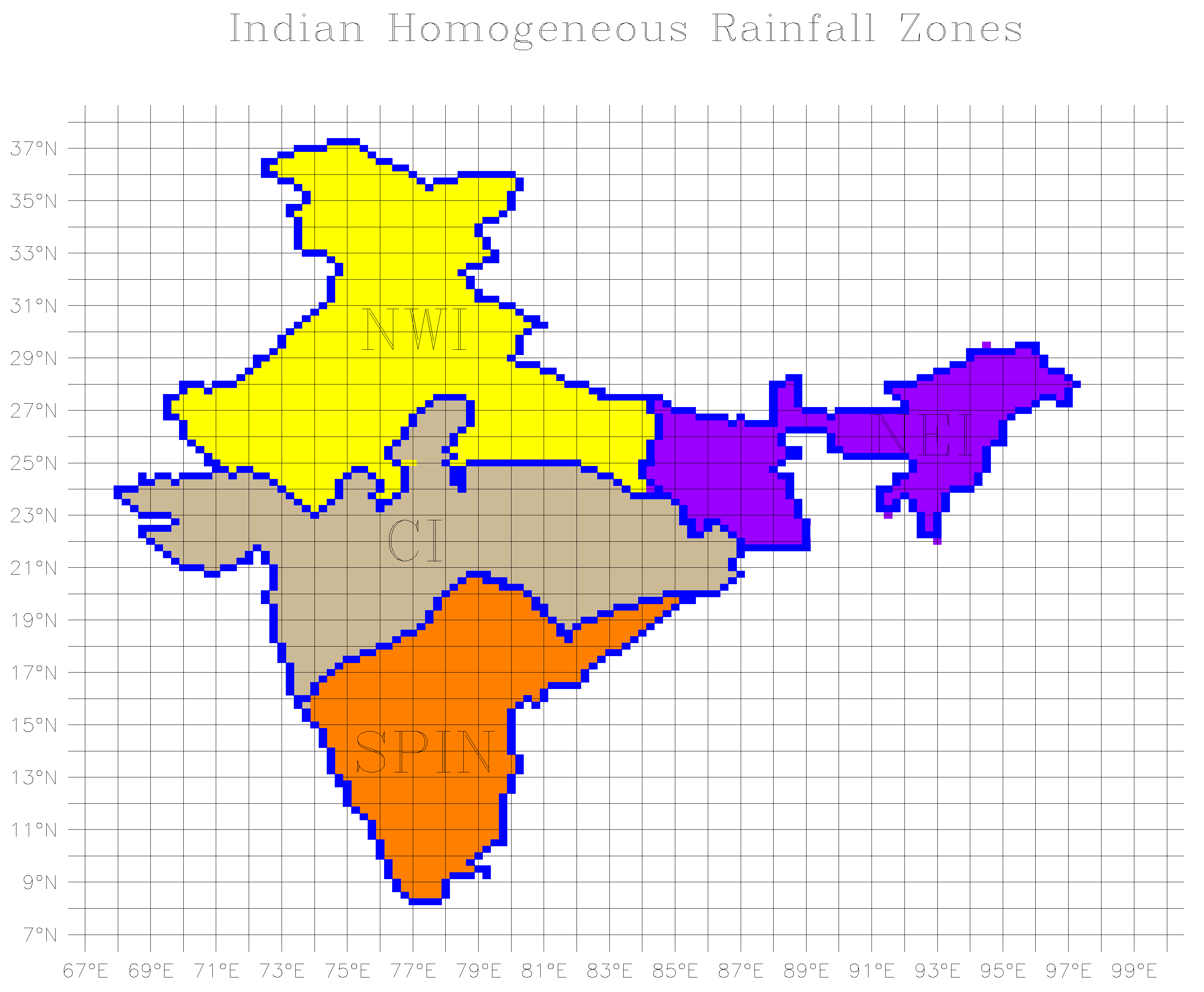
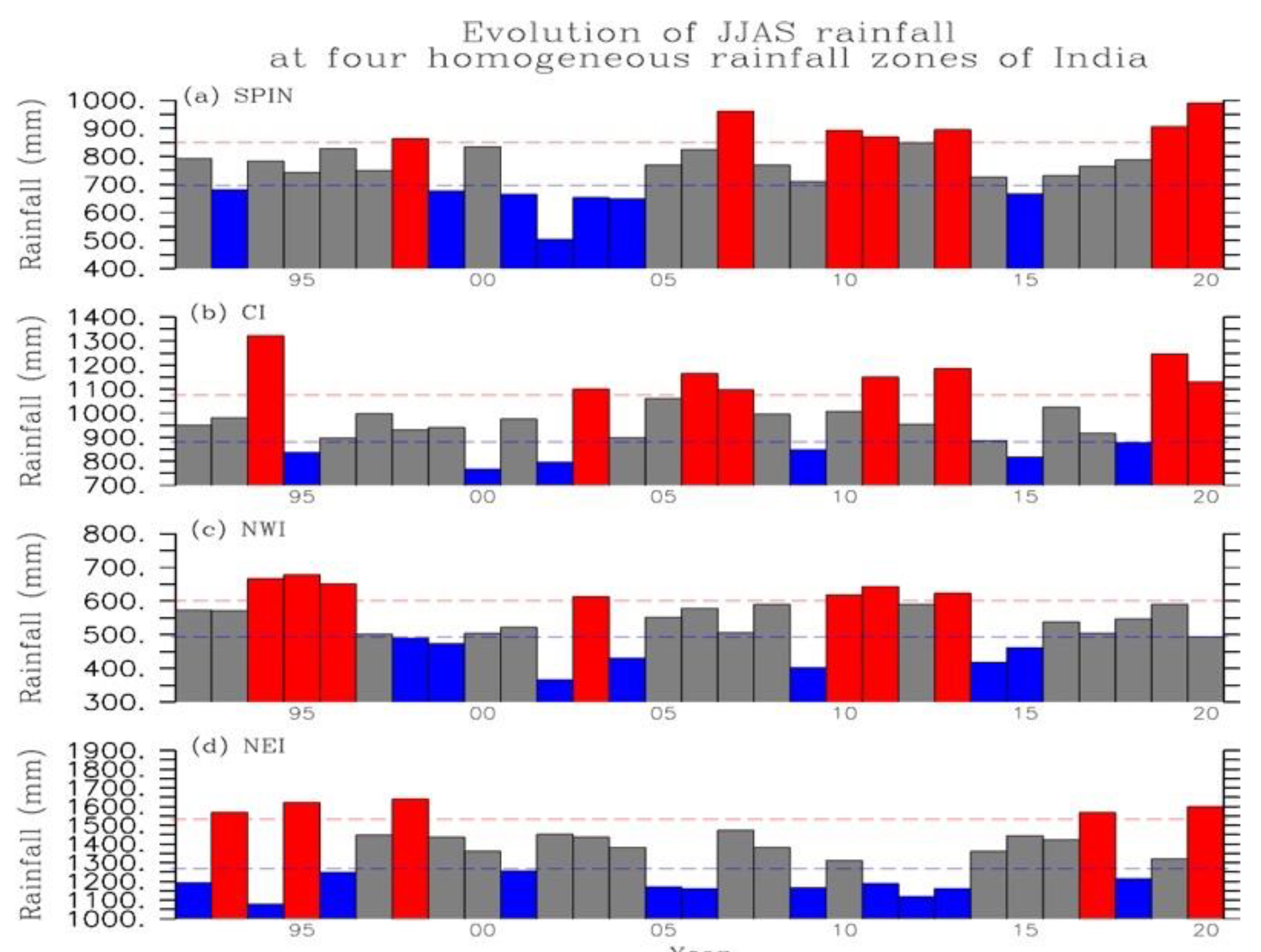
2.2. Definition of the Strength of ISMs over the IMD Regions

In this study, the classification of strong/weak ISMs was performed on regional scales owing to spatial variability in Indian rainfall. Therefore, the strength of Indian summer monsoon rainfall over an IMD region is measured by the magnitude of ISMR, which is computed as the sum of the IMD’s gridded daily rainfall area-averaged over this IMD region from 1 June through 30 September, hereafter referred to as JJAS rainfall. A strong (weak) ISM over an IMD region is when the ISMR is 10% more (less) of the JJAS rainfall climatology computed in this region over 1951–2020. This definition is consistent with the IMD-defined category “excess” (“deficient”) of Indian summer monsoon rainfall on an all-India scale (https://vajiramias.com/current-affairs/long-period-average-lpa/5cb5800c1d5def05e9b747c8/, accessed on 7 August 2022). Figure 2 illustrates the JJAS rainfall in four IMD regions during 1992–2020, with strong and weak ISMs identified according to the above definition. The years of strong, weak, and normal ISMs for each IMD region are listed in Table 1 based on Figure 2.

2.3. Summary of Methods

Observed features of SM during strong and weak ISM years are captured using a composite approach. The composite approach is generally useful for identifying the dominant features that have the potential to behave similarly and are likely governed by the same mechanisms. To examine the relation between daily SM and rainfall at each grid point, we conducted a linear correlation analysis between daily SM and daily rainfall to capture the spatial pattern of correlation across India for strong, weak, and normal rainfall over the IMD regions. A statistical significance test at a 95% confidence level for all linear correlation analysis will be conducted to examine whether the correlation is significantly different from zero. To further reduce the possible effect of runoff (i.e., TR in Equation (1)), a linear correlation is applied to daily SM and daily rainfall averaged over each IMD region for months from May through September to capture the association of daily SM with daily rainfall (Section 3.2.1). A linear regression method is used to obtain the explained variance of daily SM by daily rainfall averaged over each IMD region for each month from May through September (Section 3.2.2). We further use a linear regression method to identify how daily SM responds to the daily rainfall across India (Section 3.2.3). Autocorrelation analysis for daily SM was conducted to examine the persistence of daily SM on short timescales in each month from May through September over each IMD region during strong, weak, and normal ISM years (Section 3.2.4).

3. Results

3.1. Distinctive Features of SM between Strong and Weak ISMs

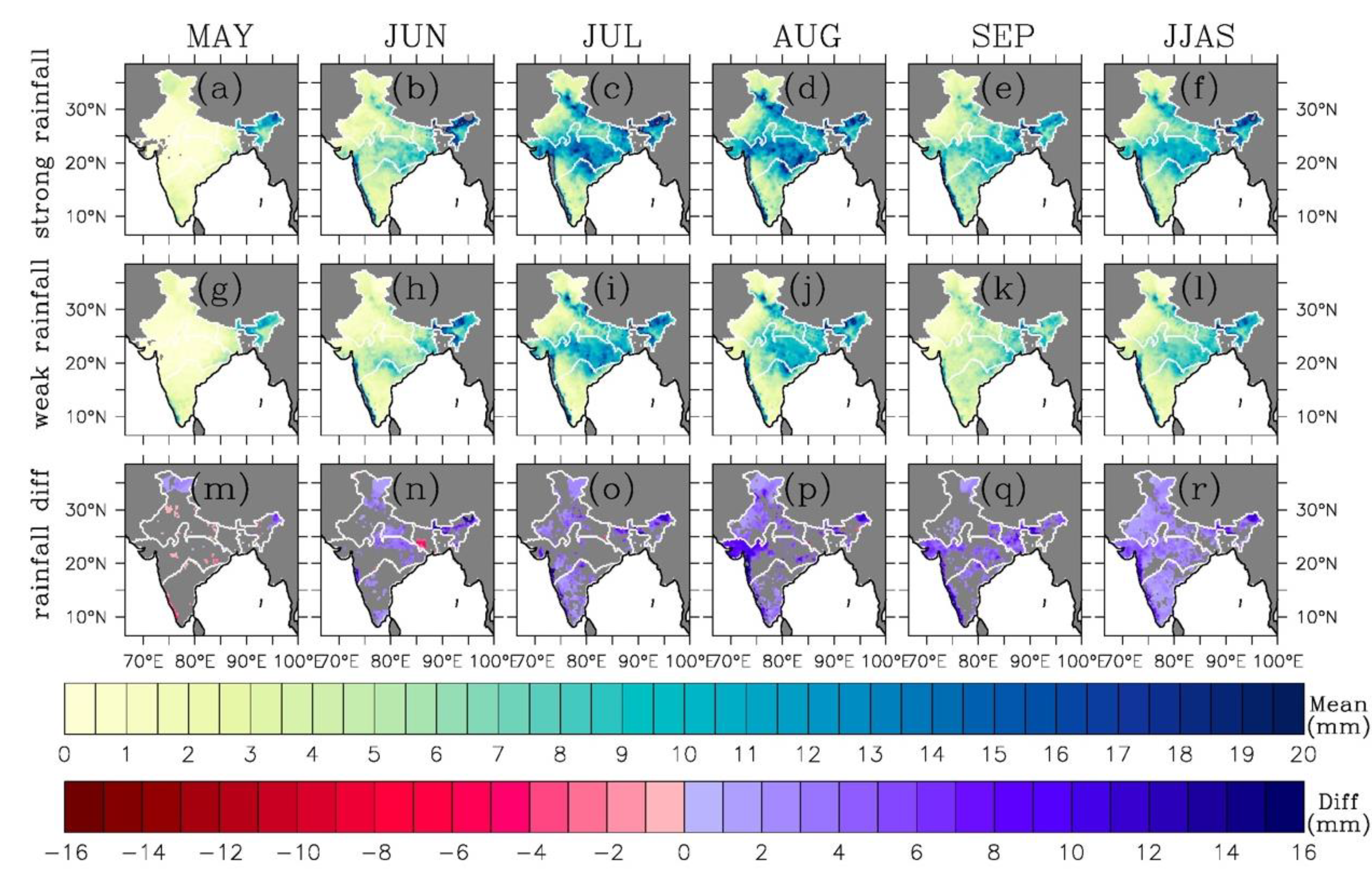
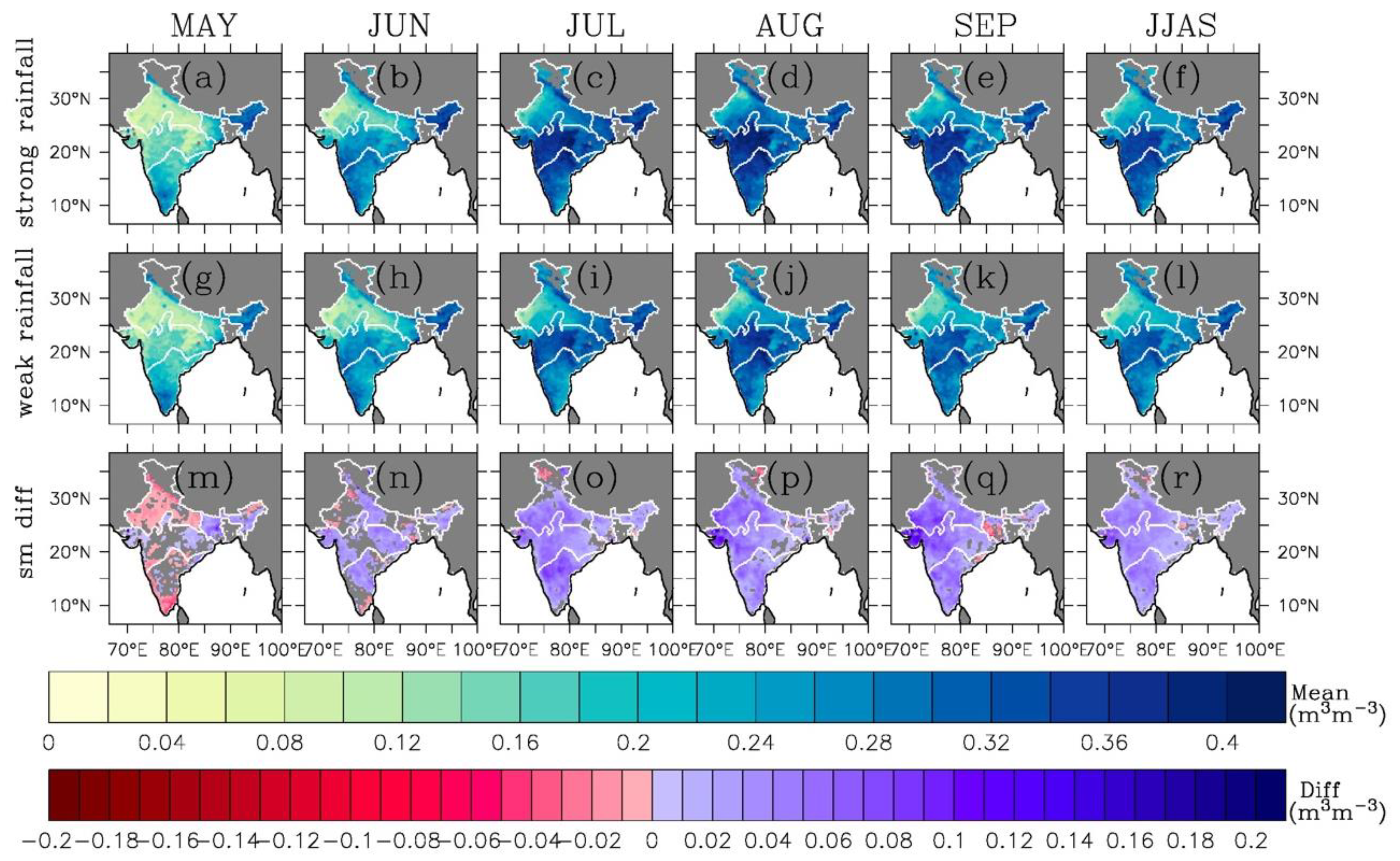
3.1.1. Spatial Distribution of Indian SM and Rainfall

Initially, we examine the spatial distribution of monthly mean (May through September) and JJAS-mean SM across the IMD regions and its association with the different strengths of rainfall. Figure 3 and Figure 4 demonstrate the monthly mean and JJAS-mean SM and rainfall between strong and weak ISMs and their differences (strong minus weak ISMs), respectively. Note that the monthly mean and JJAS-mean rainfall and SM for strong and weak ISMs were first computed for each IMD region based on the years of strong and weak ISMs for each IMD region (Table 1), then the spatial distribution of four IMD regions is combined as one map.
There are several common features for both strong and weak ISMs. First, there is no significant amount of rainfall in most of the area of India in May before the onset of ISMs except for the NEI region, thus there is little SM concurrently, with the least SM in NWI and CI. Second, in June, the onset of ISMs provides a limited amount of rainfall in SPIN and CI, which causes SM to increase gradually, mostly in SPIN and CI. Third, during the mature phase of ISMs (July and August), frequent and heavy rainfall causes SM to increase and even get saturated in some regions (mostly in CI and NEI). However, in July and August, SPIN and the west of NWI do not receive significant rainfall when monsoon rainfall is mostly located in CI and NEI due to the northward propagation of monsoonal rainband, thus, SM in west of NWI and SPIN is small compared to CI and NEI. Finally, during the withdrawal phase, the rainfall and SM become weak across India, including CI and NEI.
The differences in monthly mean SM across India are clear between strong and weak ISMs. Monthly rainfall differences in large parts of India between strong and weak ISMs are not statistically significant at a 95% confidence level (row 3 in Figure 3). As seen in the subsequent section (Section 3.1.2), the discrepancy in the evolution of daily rainfall between strong and weak ISMs is clear. We hypothesize that it is the discrepancy of short-term rainfall variation that causes the difference in daily SM between strong and weak ISMs, as will be confirmed in Section 3.2.

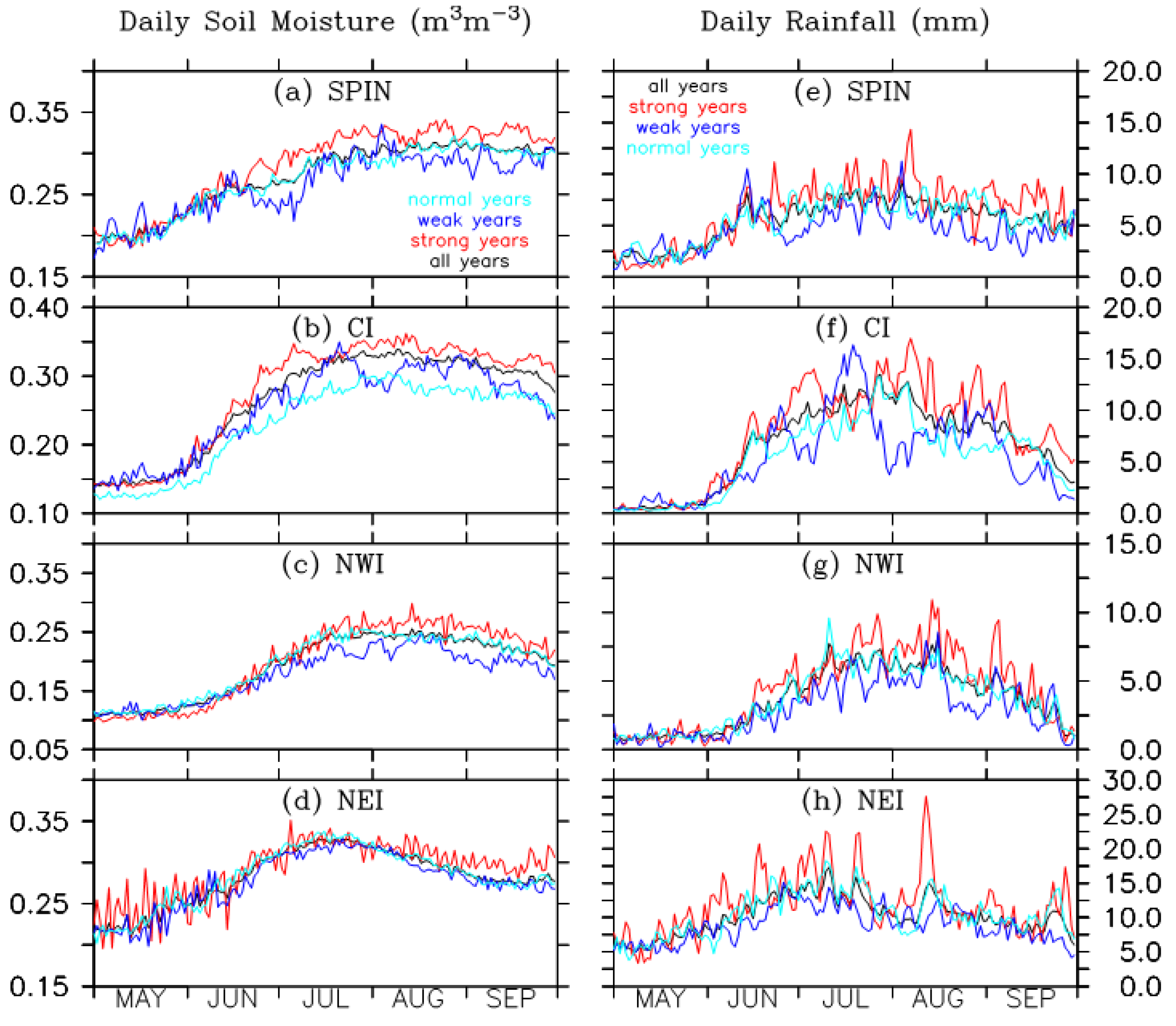
3.1.2. Temporal Distribution of Indian SM and Rainfall

Figure 5 displays the evolution of daily SM (left) and daily rainfall (right) averaged over the four IMD regions from May through September composited from strong, weak, normal ISM years and all years, respectively. It is evident that SM in the four IMD regions is overall larger (smaller) than the daily climatology over June through September during strong (weak) ISM years. SM values in May (pre-monsoon) and early June are expected to be small prior to the onset of monsoon. Figure 5e–h is the same as Figure 5a–d except for the daily rainfall. The evolution of daily SM in each IMD region is almost synchronous with the evolution of daily rainfall in the same region during strong and weak ISMs. However, the magnitude in SM change is not always consistent with the rainfall intensity. For example, large variations of SM in May in NEI occur without strong rainfall intensity. Small variations in July and August occur when rainfall is large. These results suggest that the relationship between SM and rainfall is complex and other factors also play a role as will be discussed in Section 4.

3.2. SM Dependence on Rainfall Associated with the Strength of ISMs

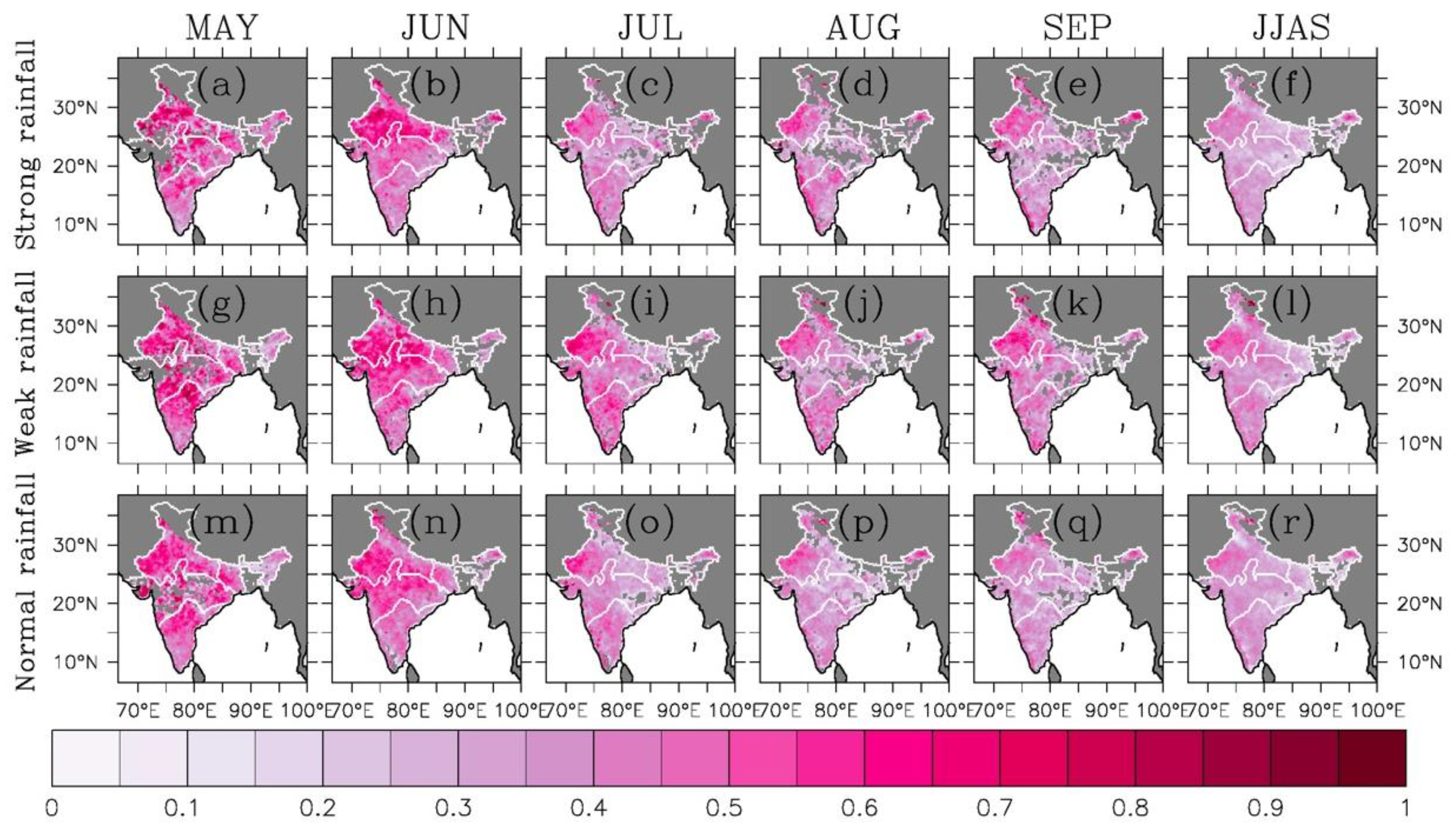
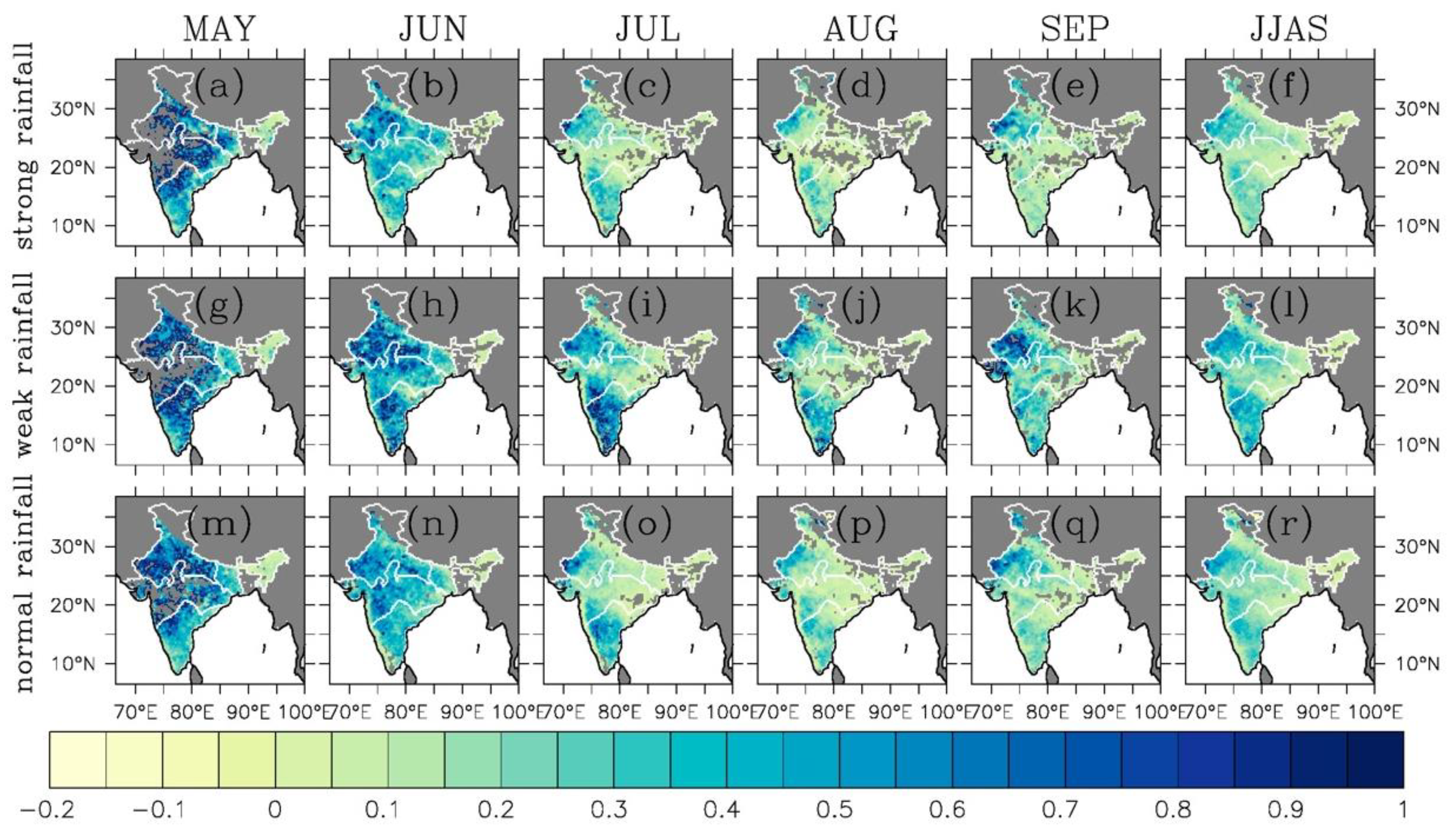
3.2.1. Spatial Distribution of Correlation between Daily SM and Daily Rainfall

Since rainfall is one of the primary sources for a change in SM, the SM content is expected to be strongly dependent on the strength of rainfall in India. It should be noted that SM content is also closely related to the soil and vegetation types, wind, and temperature conditions that determine evapotranspiration and runoff. Evapotranspiration is the primary sink (it reduces SM, but less significantly in areas with vegetation), and runoff can be sink or source for SM and is dependent on rain rate and pre-existing SM. Herein, we focus on the dependence of SM on rainfall alone, assuming that rainfall is an independent field to other factors, such as evapotranspiration, wind speed, surface and air temperature, surface water vapor, and air water vapor on these timescales. Therefore, simple linear analysis between daily SM and rainfall is appropriate.
Figure 6 shows the spatial distribution of correlation coefficient between daily SM and daily rainfall during May, June, July, August, September, and JJAS for strong, weak, and normal ISMs and only shows those which are significant at a 95% confidence level. The correlation at a location is computed only when rainfall and SM data are available at this location since rainfall is not likely to occur everywhere for all days, and since SM data at a specific location may be missing due to gaps in satellite coverage. The association of daily SM with daily rainfall depends on geographic locations for each month, consistent with the study by Sathyanadh et al. (2016) [8]. Strong correlation mostly occurs in SPIN and NWI for all months where the daily SM value is small (Figure 4), while weak correlation mostly occurs in CI and NEI for all months where the daily SM value is large (Figure 4). Moreover, it shows that the correlation is overall weak during strong ISMs than during weak ISMs, suggesting that the relationship between daily SM and daily rainfall depends on the strength of ISMs. Correlation in most of the area of NEI during July through September is generally weak for strong, weak, and normal ISMs due to its large SM during these months. Note that the above spatial pattern of correlation between daily SM and daily rainfall might be contaminated due to the 3-h time difference of defined daily values between IMD daily rainfall and ESA CCI daily SM products, as previously indicated in Section 2.1.
Some spatial averaging may help reduce the influence of runoff on SM. Therefore, to reduce the effect of runoff on the SM dependence on rainfall, we focus on the SM dependence on rainfall based on SM and rainfall spatially averaged over the IMD regions. For this purpose, we further compute the correlation between daily SM and daily rainfall averaged over the four IMD regions. Table 2 lists the summary of results. Except for NEI during May, July–August of strong ISMs, the correlation based on regionally averaged data is mostly statistically significant at a 95% confidence level regardless of the rainfall strength, suggesting the strong dependence of daily SM on daily rainfall at regional scales.

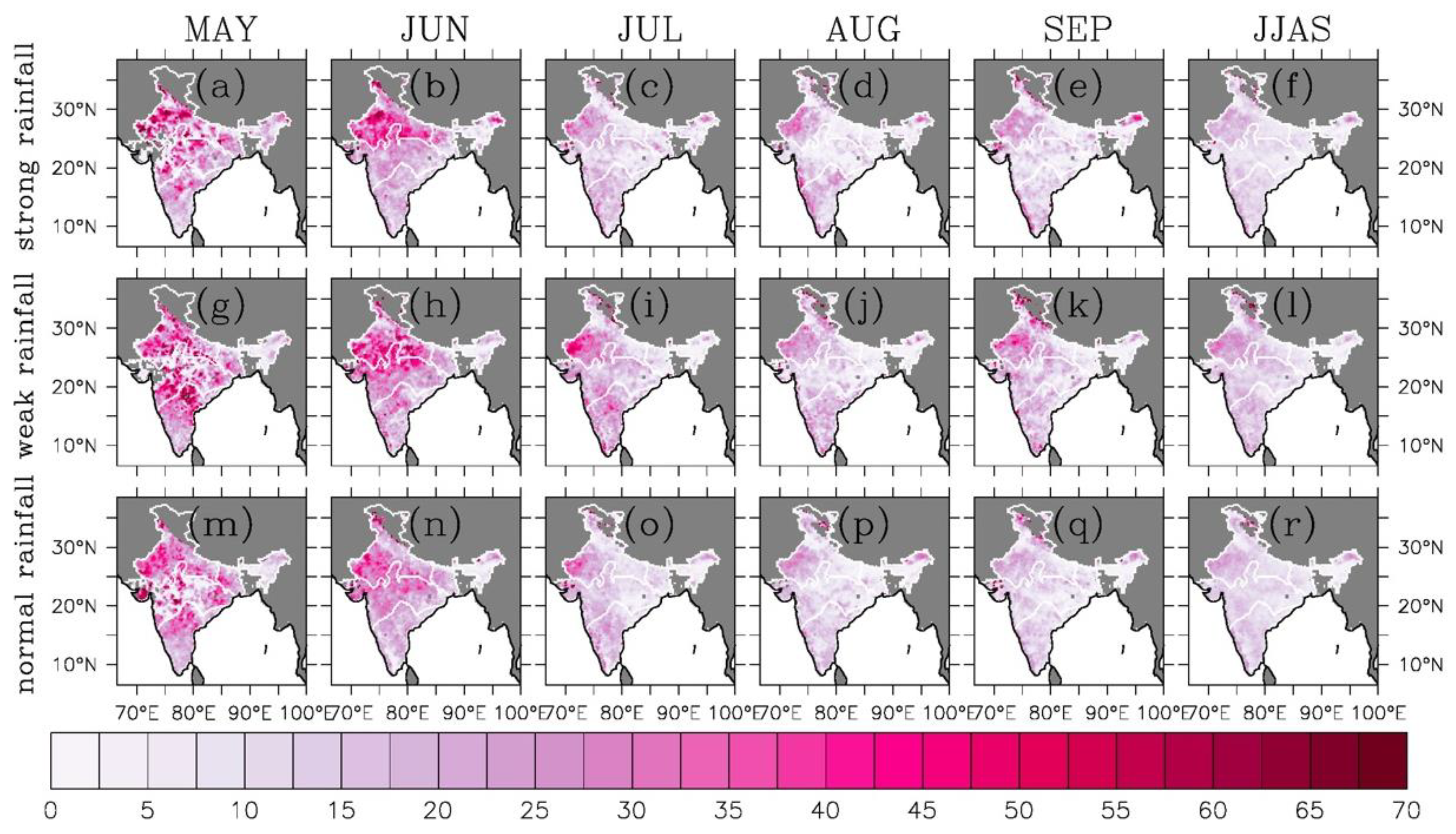
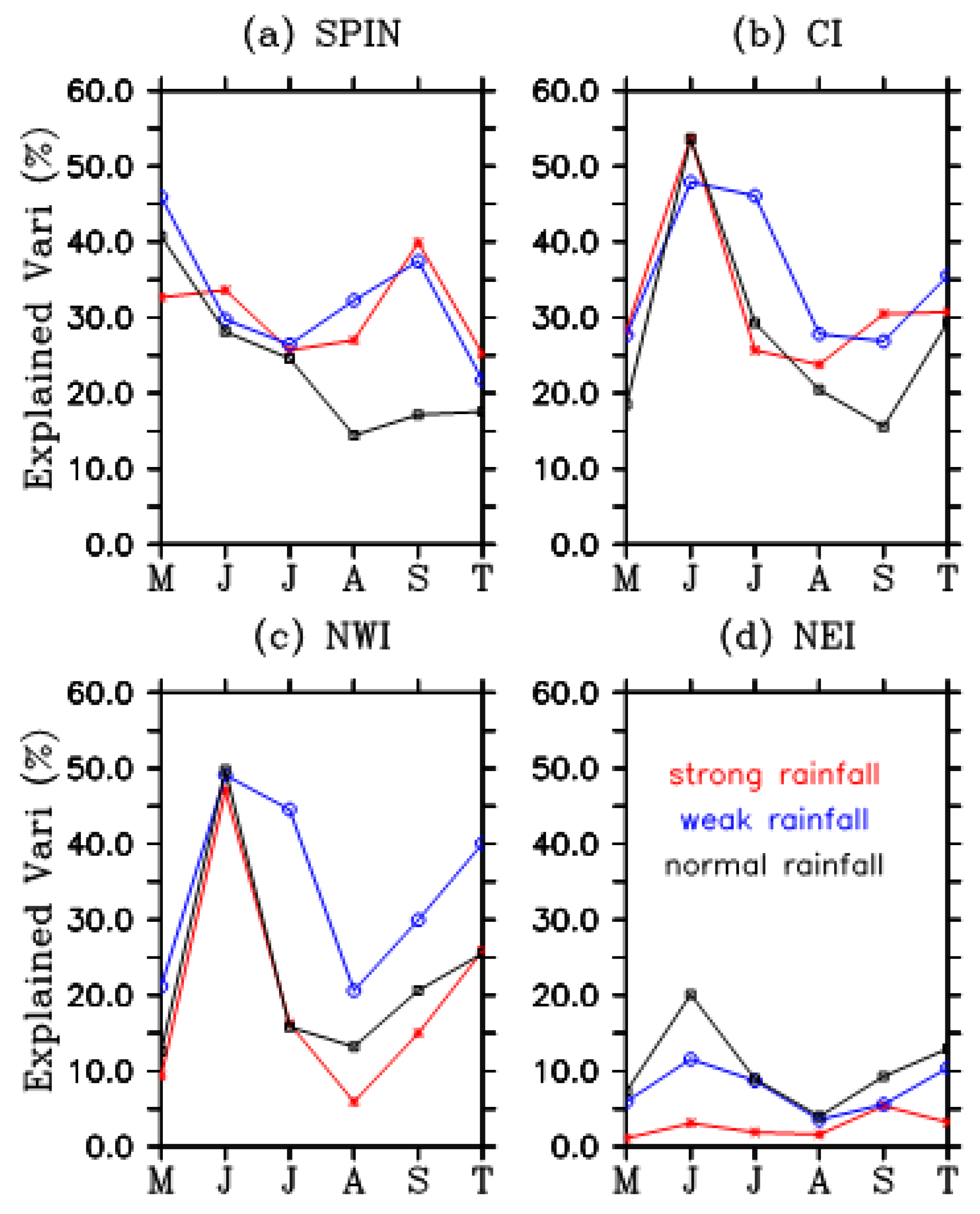
3.2.2. Explained Variance of Daily SM by Daily Rainfall

The contribution of daily rainfall to daily SM variance at each grid is measured by the explained variance of daily SM by daily rainfall using R-squared values from linear regression analysis. The spatial distribution of the explained variance during each month of May through September among strong, weak, and normal ISMs is exhibited in Figure 7. The explained variance of daily SM by daily rainfall in May is also shown here for the pre-monsoon period. Figure 7 interprets how much of daily SM variance at a location can be explained by daily rainfall at this location. The rainfall-explained variance in May is large (particularly in SPIN) but appears more scattered in space than other months. It represents the impact of scattered rainfall during the pre-monsoon period. After the onset of ISMs in June, the daily rainfall makes large contributions (up to ~70%) to daily SM variance in most of the area of India, with the largest contribution over NWI. Note that the explained variance in SPIN is relatively small in June than in May. During weak ISMs, the rainfall-explained variance in NWI and SPIN is still large in July, although smaller than in June. During strong ISMs, the rainfall-explained variance in July reduces significantly relative to June, particularly in most of CI and NWI. During the mature and withdrawal phases (July–September), NWI, CI, and SPIN have more area of greater rain-explained variance during weak ISMs than during strong ISMs. As a result, in these areas, rainfall makes a larger contribution to daily SM variance during weak ISMs than during strong ISMs for the JJAS period. The discrepancies in explained variance for each month between the IMD regions are presumably associated with the monthly mean SM value for each month between the IMD regions, as shown in Figure 4.
Figure 8 exhibits the explained variance when daily SM and daily rainfall are spatially averaged over each IMD region. In SPIN, the largest explained variance is in May during weak ISMs. In CI and NWI, the largest explained variance by rainfall occurs in June regardless of the ISM strength. In NEI, the largest explained variance occurs during June of normal ISMs and the explained variance is significantly smaller for all months during strong ISMs compared to weak and normal ISMs. When spatially averaged, among the four IMD regions, CI has the largest explained variance (~53%) during June. This suggests that the total contribution from other factors, such as soil and vegetable types, influence of runoff as well as evapotranspiration processes by environmental conditions (i.e., air temperature, wind speed, etc.) can explain about 50% of daily SM variance. Therefore, other factors also play an important role in daily SM variance, which are not addressed in this study.
Nevertheless, Figure 7 and Figure 8 imply our hypothesis that factors other than rainfall, such as evapotranspiration and runoff processes also play a role in determining the SM, which should not be ignored to fully understand the causes of SM variability on small scales. This analysis is beyond the scope of this study and would be complicated by the temporal sampling (e.g., only early in the day, only late in day, perhaps two times a day from satellites), which could make a substantial contribution to the unexplained variance.

3.2.3. Spatial Variations in Response of Daily SM to Daily Rainfall

To examine how daily SM responds to daily rainfall, the daily SM (a dependent variable) is regressed onto the daily rainfall (as an independent variable) over each month and the entire monsoon season during strong, weak, and normal ISMs, respectively. Figure 9 displays the spatial distribution of slope of linear regression at each grid across India and highlights the slope which is statistically significant at a 95% confidence level using the two-tailed student-t test. The dependence of daily SM on daily rainfall in May is strong in some portions of India (i.e., SPIN, east of CI, and some portions of NWI and NEI). This is due to the fact that there is very little moisture (Figure 4) in the soil before the onset of ISMs, in addition to the infrequent and scattered rainfall in May (Figure 3), and SM change is very sensitive to rainfall although it occurs infrequently (Figure 3). This high dependence continues and expands in a very large portion of India during June. This occurs since there is still little moisture in the soil in June (Figure 4), but with more frequent rainfall after the onset of ISMs (Figure 3). The dependence of daily SM on daily rainfall after June tends to be weak, and the strong response is located only in relatively small portions of India (west of NWI and some part of SPIN) where SM is still relatively small (Figure 4).
The small response of daily SM to daily rainfall after June is partly due to the fact that SM is large and/or saturated or near saturated in some portions of India (Figure 4), and it cannot vary significantly although more frequent and heavy rainfall occurs. Particularly, the response of daily SM to daily rainfall is weak and not significant in most of CI and NEI since daily SM is already large (Figure 3). Due to varied climatic conditions, India has different types of soils varying from Alluvial soils to mountain soils. Similarly, India has a wide range of natural vegetation as well, varying from tropical evergreen forests to mangroves. In addition, different crops are grown depending upon the season and soil types. Therefore, the above spatial variations in linear response can be affected by local soil, landscape, and vegetation types as well as environmental conditions (wind speed, surface temperature, and air temperature above surface, etc.), which is beyond the scope of this study. At the same locations, it is also evident that there are overall stronger responses of daily SM to daily rainfall during weak ISMs than during strong ISMs. The responses during normal ISMs seem to be in-between the responses for the extremes. The strongest responses occur in June (June–July) for strong (weak) ISMs in large parts of India during which the daily SM variance is highly explained by daily rainfall (Figure 7 and Figure 8) and the regions of strong responses are relatively smaller in other months. The different responses between months as well as between strong, weak, and normal ISMs represent the impact of daily rainfall on daily SM on the daily basis and factors other than rainfall come to play a role in daily SM. Compared to Figure 4, we find that the locations of strong responses are overall the locations where SM is small (e.g., SPIN, NWI), while the locations of weak responses are overall the locations where SM is large (e.g., CI, NEI), suggesting the importance of the prior state of daily SM value to its dependence on daily rainfall. However, whether daily SM can reduce quickly or not is closely tied to SM persistence, which can be controlled by the rainfall and other factors, such as soil and vegetation types, winds, surface and air temperature, air water vapor, etc. The persistence of SM in the four IMD regions is discussed in Section 3.2.4.

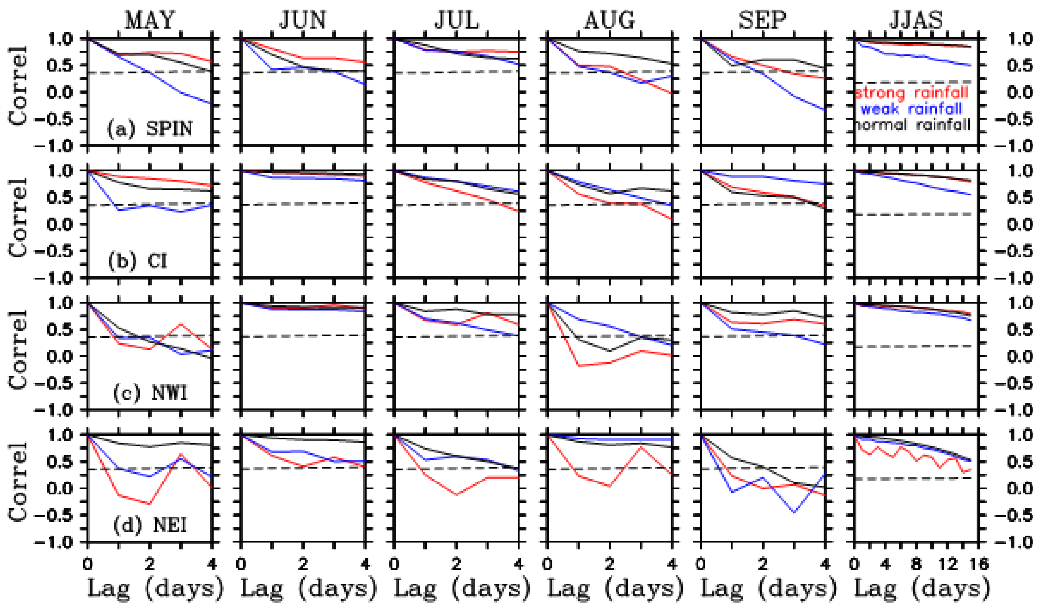
3.2.4. Persistence in Daily SM

The SM state at one location can be less changed between adjacent days due to its strong persistency, which can be caused by rainfall input or factors other than rainfall, such as meteorological and environmental conditions. Figure 10 shows the lag autocorrelation of daily SM averaged over the four IMD regions for each month from May through September and JJAS period and they are compared among strong, weak, and normal ISMs. The lag at which the correlation value falls below the 95% confidence level reflects the SM persistence. The results represent the SM persistence on short timescales rather than on intraseasonal and seasonal timescales if the lags are several days only.
The SM persistence is closely related to the prior magnitude of SM value and subsequent short-term rainfall fluctuations: Small SM tends to have a weak persistence with small rainfall fluctuations and large SM tends to have a strong persistence with small variations of strong rainfall. For example, SM in May in NWI, usually small (Figure 4) with small rainfall fluctuations (Figure 5), tends to have a short persistence (around 1–2 days) during weak ISMs. SM in CI in June tends to have a long persistence partly since there is a trend of increase in rainfall. However, SM in July and August is usually large (Figure 4 and Figure 5), but it tends to have a short persistence. This happens probably due to large short-term rainfall fluctuations (Figure 5) and/or other factors than rainfall play an important role. SM in NEI is large but has weaker persistence during strong ISMs than weak ISMs (Figure 10d) probably also due to stronger rainfall fluctuations (Figure 5h), particularly in May. When computed over the entire ISM period (i.e., JJAS), except in NEI, normal ISMs generally have the strongest daily SM persistence, weak ISMs have the weakest daily SM persistence, and daily SM persistence during strong ISMs is in-between. Note that other factors, such as runoff and agricultural use of water (e.g., irrigation) also affect daily SM persistence on small spatial scales. However, the effect of runoff on SM daily persistence can be greatly reduced when spatially averaged over the entire India and four IMD regions. Therefore, the stronger spatially averaged SM daily persistence during strong ISMs relative to weak ISMs shown in Figure 10 may not be primarily due to runoff. How the agriculture uses of water, such as irrigation can affect daily SM persistence at national and regional levels is unknown and beyond the scope of this study. Nevertheless, Figure 10 does show that daily rainfall fluctuations at short-time scales play a role in short-term daily SM persistence.

4. Discussion

It is well known that in addition to rainfall, SM is affected by other factors, such as runoff, environmental, and meteorological conditions (soil and vegetation types, surface air temperature, water vapor mixing ratio, wind speed, etc.) influencing the evapotranspiration process, which are not investigated in this study. Some of these factors have been investigated by other studies. For example, Pangaluru et al. (2019) [11] suggested that SM variability is associated with surface air temperature. Other atmosphere fields, such as water vapor mixing ratio and wind speed can affect SM variability through influencing the evapotranspiration processes. Agricultural use of water, such as irrigation can also influence SM in India at some spatial scales, particularly in the regions experiencing droughts. Note that the dependence of SM on rainfall can be reduced by the strong SM persistence, particularly when SM is close to near saturation or saturation and SM persistence is also closely tied to soil and vegetation types, runoff, and meteorological conditions. Therefore, the dependence of SM on rainfall during the ISM years found in this study should be justified by taking these mixed factors into account. To rule out some of these effects, we have investigated the characteristics of SM persistence in the four IMD regions in each month for strong, weak, and normal ISMs based on daily SM. We also reduced the potential effects of runoff on SM by performing spatial averaging over each of the four IMD regions.
The SM conditions in pre-monsoon periods affect SM content during early ISM seasons, which is attributed to SM persistence and may affect SM content over the entire ISM seasons since pre-monsoon SM conditions influence the ISM onset and precipitation [21]. Nevertheless, the short-term SM fluctuations in NWI, CI, and SPIN are overall dependent on the short-term rainfall variations in June of strong and in June–July of weak ISMs. Since strong SM persistence plays an important role in modulating the dependence of SM on rainfall on short timescales, the discrepancies in SM persistence between strong and weak ISMs (Figure 10) partly explain the distinct dependencies of SM on rainfall at regional scales. Another intriguing question is concerning the SM persistence if the SM averaged from root zone to surface was computed. Since the ESA CCI SM product used in this study represents the SM averaged in the top 10 cm only, shallower than the root zone, it cannot be used to directly address the above question. However, since the SM persistence is generally increased with soil depth [22], the SM persistence averaged from root zone to surface is expected to be stronger than what we find in this study. Despite the different strengths of ISMs, the SM features are truly affected at least by rainfall features for each region.
Note that the results in this study are obtained by assuming that other factors are independent parameters to rainfall in affecting SM variability from the perspective of statistics and mathematics. Since rainfall is the primary source of SM, it is reasonable to assume that the dependence of SM on rainfall is strong. The results found in this study based on the assumption are reasonable.

5. Conclusions

In this study, the variability of SM and its dependence on rainfall in the four Indian homogeneous rainfall zones during strong, weak, and normal ISMs are examined using the ESA CCI v06.1 gridded SM combined product and the IMD’s daily 0.25° gridded rainfall product over the period 1992–2020.
The three major results found show that:
(1)
Monthly and seasonally mean SM values in NWI, CI, and SPIN at the same locations are generally higher during strong ISMs than during weak ISMs. The regional distinct SM features between the IMD regions are not only associated with the strength of rainfall, but presumably associated with other factors, such as local soil and vegetable types and environmental conditions (winds, surface and air temperature, air water vapor, etc.) which influence the capability of holding the SM values locally. Nevertheless, the distinct SM features at the same location between the different strengths of ISMs are associated with daily rainfall magnitude and its short-term fluctuations.
(2)
The daily SM and its dependence on daily rainfall appear to be region-locked in space and phase-locked in time: Strong correlation and large response generally occur in most parts of SPIN and NWI during June (June–July) of strong (weak) ISMs where SM values are relatively small; Weak correlation and weak response generally occur in CI and NEI in July-September (August–September) of strong (weak) ISMs where SM values are relatively large. The region-locked feature is presumably associated with the local soil and vegetation types and/or environmental conditions. The phase-locked feature is associated with the features of ISMs.
(3)
Daily SM persistence in each IMD region is not only controlled by the strength of ISMs and short-term rainfall fluctuations in each IMD region, but is strongly associated with previous SM values, which are presumably tied with the local features, such as soil and vegetation types and/or environmental conditions.
As mentioned earlier, a complete understanding of SM change mechanisms needs to consider the impacts of other factors, such as soil and vegetation types, runoff, agricultural use of water (e.g., irrigation), and meteorological conditions, which requires a detailed water balance study. The influences of these factors are interwoven, linking with the strength of ISMs and local soil and vegetation types. For example, the proportion of surface runoff is high due to less infiltration and percolation when the rainfall is strong during this season. The proportion of surface runoff is closely determined by the local soil and vegetation types, as well. These factors may strongly influence the SM dependence on rainfall at small scales.

Author Contributions

Conceptualization, Y.Z.; methodology, Y.Z., M.A.B., and M.M.A.; validation, M.A.B. and M.M.A.; formal analysis, Y.Z.; investigation, Y.Z., M.A.B., and M.M.A.; data curation, Y.Z.; writing—original draft preparation, Y.Z.; writing—review and editing, M.A.B. and M.M.A.; visualization, Y.Z.; funding acquisition, M.A.B. All authors have read and agreed to the published version of the manuscript.

Funding

This research was funded by the National Aeronautics and Space Administration (NASA) Physical Oceanography through the Jet Propulsion Laboratory (JPL) in support of the Ocean Vector Winds Science Team (OVWST) (NASA/JPL/OVWST/Contract # 1419699).

Data Availability Statement

IMD 0.25° daily gridded rainfall product for Indian subcontinent can be obtained at https://cdsp.imdpune.gov.in/home_gridded_data.php#griddedRainfall (accessed on 7 August 2022). The ESA CCI 0.25° daily gridded SM product can be obtained with approval on the CCI Soil Moisture project website at https://www.esa-soilmoisture-cci.org/data (accessed on 7 August 2022).

Acknowledgments

We are grateful to the India Meteorological Department, which provides the latest daily gridded rainfall data. We also greatly appreciate the European Space Agency (ESA) for providing the ESA Climate Change Initiative (CCI) 0.25° × 0.25° gridded daily SM combined product version 06.1 data, which can be found at https://www.esa-soilmoisture-cci.org/data. The Center for Ocean-Atmospheric Prediction Studies (COAPS) at the Florida State University provided the computational facilities for this study. The present study is fully supported by the NASA Physical Oceanography in support of the Ocean Vector Winds Science Team (OVWST), NASA NEWS, and the NOAA Climate Observing Division (COD).

Conflicts of Interest

The authors declare no conflict of interest.

References

  1. Kerr, J.M. Sustainable Development of Rainfed Agriculture in India (No. 20); International Food Policy Research Institute (IFPRI): New Delhi, India, 1996. [Google Scholar]
  2. Wuttichai, G.; Kosittrakun, M.; Righetti, T.L.; Weerathaworn, P.; Prabpan, M. Normalized difference vegetation index relationships with rainfall patterns and yield in small plantings of rainfed sugarcane. AJCS 2011, 5, 1845–1851. [Google Scholar]
  3. Dutta, D.; Kundu, A.; Patel, N.R.; Saha, S.K.; Siddiqui, A.R. Assessment of agricultural drought in Rajasthan (India) using remote sensing derived Vegetation Condition Index (VCI) and Standardized Precipitation Index (SPI). Egypt. J. Remote Sens. Space Sci. 2015, 18, 53–63. [Google Scholar] [CrossRef]
  4. Guhathakurta, P. Drought in districts of India during the recent all India normal monsoon years and its probability of occurrence. Mausam 2003, 54, 542–545. [Google Scholar] [CrossRef]
  5. Robock, A.; Vinnikov, K.Y.; Srinivasan, G.; Entin, K.; Hollinger, S.E.; Speranskaya, N.A.; Liu, S.; Namkhai, A. The global soil moisture data bank. Bull. Am. Meteor. Soc. 2000, 81, 1281–1299. [Google Scholar] [CrossRef]
  6. Koster, R.D.; Guo, Z.; Yang, R.; Dirmeyer, P.A.; Mitchell, K.; Puma, M.J. On the nature of soil moisture in land surface models. J. Climate 2009, 22, 4322–4335. [Google Scholar] [CrossRef]
  7. Liu, Y.Y.; Parinussa, R.M.; Dorigo, W.A.; De Jeu, R.A.M.; Wagner, W.; van Dijk, A.I.J.M.; McCabe, M.F.; Evans, J.P. Developing an improved soil moisture dataset by blending passive and active microwave satellite-based retrievals. Hydrol. Earth Syst. Sci. 2011, 15, 425–436. [Google Scholar] [CrossRef]
  8. Sathyanadh, A.; Karipot, A.; Ranlkar, M.; Prabhakaran, T. Evaluation of soil moisture data products over Indian region and analysis of spatio-temporal characteristics with respect to monsoon rainfall. J. Hydrol. 2016, 542, 47–62. [Google Scholar] [CrossRef]
  9. Liu, D.; Yu, Z.; Mishra, A.K. Evaluation of soil moisture-precipitation feedback at different time scales over Asia. Int. J. Climatol. 2017, 37, 3619–3629. [Google Scholar] [CrossRef]
  10. Shrivastava, S.; Kar, S.C.; Sharma, A.R. Soil moisture variations in remotely sensed and reanalysis datasets during weak monsoon conditions over central India and central Myanmar. Theor. Appl. Climatol. 2017, 129, 305–320. [Google Scholar] [CrossRef]
  11. Pangaluru, K.; Velicogna, I.; Mohajerani, G.A.Y.; Ciraci, E.; Charakola, S.; Bahsa, G.; Rao, S.V.B. Soil moisture variability in India: Relationship of land surface-atmosphere fields using maximum covariance analysis. Remote Sens. 2019, 11, 335. [Google Scholar] [CrossRef]
  12. Singh, R.P.; Mishra, D.R.; Shaoo, A.K.; Dey, S. Spatial and temporal variability of soil moisture over India using IRS P4 MSMR data. Int. J. Remote Sens. 2005, 26, 2241–2247. [Google Scholar] [CrossRef]
  13. Zheng, Y.; Bourassa, M.A.; Ali, M.M.; Krishnamurti, T.N. Distinctive features of rainfall over the Indian homogeneous rainfall regions between strong and weak Indian summer monsoons. J. Geophys. Res. Atmos. 2016, 121, 5631–5647. [Google Scholar] [CrossRef]
  14. Zheng, Y.; Ali, M.M.; Bourassa, M.A. Contribution of monthly and regional rainfall to the strength of Indian summer monsoon. Mon. Weather Rev. 2016, 144, 3037–3055. [Google Scholar] [CrossRef]
  15. Zheng, Y.; Bourassa, M.A.; Ali, M.M. Statistical evidence on distinct impacts of short- and long-time fluctuations of Indian Ocean surface wind fields on Indian summer monsoon rainfall during 1991–2014. Clim. Dyn. 2020, 54, 3053–3076. [Google Scholar] [CrossRef]
  16. Pattanik, D.R. Analysis of rainfall over different homogeneous regions of India in relation to variability in westward movement frequency of monsoon depressions. Nat. Hazards 2007, 40, 635–646. [Google Scholar] [CrossRef]
  17. Pai, D.S.; Sridhar, L.; Rajeevan, M.; Sreejith, O.P.; Satbhai, N.S.; Mukhopadhyay, B. Development of a new high spatial resolution (0.25° × 0.25°) long period (1901–2010) daily gridded rainfall data set over India and its comparison with existing data sets over the region. Mausam 2014, 65, 1–18. [Google Scholar]
  18. Scanlon, T.; Pasik, A.; Dorigo, W.; de Jeu, R.A.M.; Hahn, S.; van der Schalie, R.; Wagner, W.; Kidd, R.; Gruber, A.; Moesinger, L.; et al. Algorithm Theoretical Basis Document (ATBD) Supporting Product Version 06.1; Deliverable 2.1 Version 2; Earth Observation Data Centre for Water Resources Monitoring (EODC) GmbH: Zürich, Switzerland, 2021. [Google Scholar]
  19. Gruber, A.; Scanlon, T.; van der Scalie, R.; Wagner, W.; Dorigo, W. Evolution of the ESA CCI Soil Moisture climate data records and their underlying merging methodology. Earth Syst. Sci. Data 2019, 11, 717–739. [Google Scholar] [CrossRef]
  20. Dorigo, W.A.; Wagner, W.; Albergel, C.; Albrecht, F.; Balsamo, G.; Brocca, L.; Chung, D.; Ertl, M.; Forkel, M.; Gruber, A.; et al. ESA CCI Soil Moisture for improved Earth system understanding: State-of-the art and future directions. Remote Sens. Environ. 2017, 203, 185–215. [Google Scholar] [CrossRef]
  21. Asharaf, S.; Dobler, A.; Ahrens, B. Soil moisture-precipitation feedback processes in the Indian summer monsoon season. J. Hydrometeor. 2012, 13, 1461–1474. [Google Scholar] [CrossRef]
  22. Asharaf, S.; Ahrens, B. Soil-moisture memory in the regional climate model COSMO-CLM during the Indian summer monsoon season. J. Geophys. Res. Atmos. 2013, 118, 6144–6151. [Google Scholar] [CrossRef]
Figure 1. Map of the four Indian homogeneous rainfall zones projected on 0.25° × 0.25° daily rainfall grids used in this study. NWI, CI, SPIN, and NEI are shown in yellow, tan, orange, and purple, respectively. The borders between each IMD region are shown in blue.
Water 14 02788 g001
Figure 2. Evolution of JJAS Indian rainfall (in mm) over (a) SPIN, (b) CI, (c) NWI, and (d) NEI for the period 1992–2020 derived from the daily 0.25° gridded rainfall product provided by IMD. Strong (red bars), weak (blue bars), and normal (gray bars) ISMs are identified by the departure of JJAS rainfall of each year from the JJAS rainfall climatology computed over each IMD region for the period 1951–2020, whose departure values are larger than +10%, smaller than −10%, and within −10% and +10% of the seasonal climatology, respectively. The red (blue) dashed line denotes a value of 110% (90%) of seasonal climatology (i.e., the JJAS rainfall climatology for SPIN, CI, NWI, and NEI are 776.4, 979.3, 545.5, and 1397 mm, respectively).
Water 14 02788 g002
Figure 3. Spatial variations in monthly mean rainfall for May through September and JJAS-mean rainfall for strong ISMs (top row, (af)), weak ISMs (second row, (gl)), and its difference (strong ISMs minus weak ISMs) (bottom row, (mr)). The difference is shown only when it is statistically significant at a 95% confidence level. The monthly and JJAS-mean rainfall was computed based on the IMD 0.25° daily gridded rainfall. The horizontal color bar on the top and bottom denotes the mean and difference, respectively. The unit for daily rainfall is mm. The borders between the IMD regions are shown in white.
Water 14 02788 g003
Figure 4. Spatial variations in monthly mean soil moisture for May through September and JJAS-mean rainfall for strong ISMs (top row, (af)), weak ISMs (second row, (gl)), and its difference (strong ISMs minus weak ISMs) (bottom row, (mr)). The difference is shown only when it is statistically significant at a 95% confidence level. The unit for daily volumetric soil moisture is m3 m−3. The borders between the IMD regions are shown in white.
Water 14 02788 g004
Figure 5. The evolution of daily surface soil moisture (left) area averaged over (a) SPIN, (b) CI, (c) NWI, and (d) NEI and the evolution of daily rainfall (right) area averaged over (e) SPIN, (f) CI, (g) NWI, and (h) NEI from May through September for strong (red curve), weak (blue curve), normal (cyan curve) ISM years and all years (black curve). Soil moisture and rainfall daily climatology were computed based on the period 1992–2020. The unit for daily volumetric soil moisture (daily rainfall) is m3 m−3 (mm).
Water 14 02788 g005
Figure 6. Spatial distribution of correlation coefficient between daily SM and daily rainfall in India for May through September and JJAS during strong ISMs (top row, (af)), weak ISMs (second row, (gl)), and normal ISMs (bottom row, (mr)). The correlation was computed based on soil moisture grids using the IMD 0.25° grids daily rainfall and 0.25° grids daily SM. The correlation coefficient is shown only when it is significant at a 95% confidence level. The borders between the IMD regions are shown in white.
Water 14 02788 g006
Figure 7. Spatial distribution of explained variance in India based on a linear regression analysis for daily SM regressed on daily rainfall for May through September and JJAS during strong ISMs (top row, (af)), weak ISMs (second row, (gl)), and normal ISMs (bottom row, (mr)). The linear regression was computed based on the IMD 0.25° daily rainfall grids. The period for analysis is 1992–2020. The borders between the IMD regions are shown in white.
Water 14 02788 g007
Figure 8. Explained variance based on a linear regression for spatially averaged daily SM regressed on spatially averaged daily rainfall during May, June, July, August, September, and June-September (JJAS, denoted by T in x-axis) of strong (red), weak (blue), and normal (black) ISMs over (a) SPIN, (b) CI, (c) NWI, and (d) NEI.
Water 14 02788 g008
Figure 9. Spatial distribution of slope in India based on a linear regression analysis for daily SM regressed on daily rainfall for May through September and JJAS during strong ISMs (top row, (af)), weak ISMs (second row, (gl)), and normal ISMs (bottom row, (mr)). The slope at each grid is computed based on the linear regression analysis (i.e., SM = slope × rainfall + intercept). The slope is shown only when it is statistically significant at the 95% confidence level. Note that slope values have been multiplied by 100.
Water 14 02788 g009
Figure 10. Lag autocorrelation for soil moisture averaged over (a) SPIN, (b) CI, (c) NWI, and (d) NEI for May, June, July, August, September, and JJAS during strong, weak, and normal ISMs. Red, blue, and black curves represent the lag auto correlation of daily mean soil moisture for strong, weak, and normal ISMs, respectively. The day of strong SM persistence is defined as the number of lag days when the auto-correlation coefficient first falls below the critical values (dashed lines) at the 95% confidence level.
Water 14 02788 g010
Table 1. A list of years with strong, weak, and normal rainfall over SPIN, CI, NWI, and NEI for the period 1992–2020. The method to define the strength of JJAS rainfall over the IMD regions is described in Section 2.2.
LocationISM StrengthYears
SPINStrong98, 07, 10, 11, 13, 19, 20
Weak93, 99, 01, 02, 03, 04, 15
Normal92, 94, 95, 96, 97, 00, 05, 06, 08, 09, 12, 14, 16, 17, 18
CIStrong94, 03, 06, 07, 11, 13, 19, 20
Weak95, 00, 02, 09, 15, 18
Normal92, 93, 96, 97, 98, 99, 01, 04, 05, 08, 10, 12, 14, 16, 17
NWIStrong94, 95, 96, 03, 10, 11, 13
Weak98, 99, 02, 04, 09, 14, 15
Normal92, 93, 97, 00, 01, 05, 06, 07, 08, 12, 16, 17, 18, 19, 20
NEIStrong93, 95, 98, 17, 20
Weak92, 94, 96, 01, 05, 06, 09, 11, 12, 13,18
Normal97, 99, 00, 02, 03, 04, 07, 08, 10, 14, 15, 16, 19
Table 2. Correlation coefficients between daily soil moisture and daily rainfall averaged over SPIN, CI, NWI, and NEI during strong, weak, and normal ISMs. Correlation coefficient in bold font is significantly different from zero at a 95% confidence level using a two-tailed Student-t test.
LocationISM StrengthsMayJunJulAugSepJJAS
SPINStrong0.570.580.510.520.630.50
Weak0.680.550.510.570.610.47
Normal0.640.530.500.380.410.42
CIStrong0.530.730.510.490.550.55
Weak0.530.690.680.530.520.60
Normal0.430.730.540.450.390.54
NWIStrong0.310.690.400.230.390.51
Weak0.460.700.670.450.550.63
Normal0.360.710.400.360.450.53
NEIStrong0.100.17 0.14 0.13 0.230.18
Weak0.240.340.300.190.240.32
Normal0.270.450.300.200.300.36
Publisher’s Note: MDPI stays neutral with regard to jurisdictional claims in published maps and institutional affiliations.

