Article

Changes in Extreme Precipitation on the Tibetan Plateau and Its Surroundings: Trends, Patterns, and Relationship with Ocean Oscillation Factors

1
History, Culture and Tourism School, Fuyang Normal University, Fuyang 311400, China
2
Institute of Desert Meteorology, China Meteorological Administration, Urumqi 830002, China
*
Authors to whom correspondence should be addressed.
Water 2022, 14(16), 2509; https://doi.org/10.3390/w14162509
Submission received: 3 June 2022 / Revised: 3 August 2022 / Accepted: 10 August 2022 / Published: 15 August 2022
(This article belongs to the Special Issue Variations of Precipitation Extremes in Arid Regions)

Abstract

:
The Tibetan Plateau is among the region’s most sensitive areas to global climate change. The observation data from 113 meteorological stations on the Tibetan Plateau and surrounding regions in China for 1971–2017 were used to analyze the periodic oscillations and trends in precipitation and extreme precipitation on multiple time scales to ensemble empirical mode decomposition. The relationship between extreme precipitation and sea-surface temperature (SST) anomalies was also explored. The results were as follows. (1) The timing of extreme-precipitation events in the highlands is consistent, with increased total precipitation and increased frequency, intensity, and extreme values of extreme precipitation. (2) Changes in temperature and precipitation are not completely synchronized. The total extreme precipitation, number of extreme-precipitation days, maximum single-day precipitation, and extreme single-day precipitation intensity all showed increases with fluctuations; the quasi-3-year oscillation contributes the most to the extreme precipitation. PRCPTOT is most strongly correlated with R10 and R95p. (3) The spatiotemporal patterns of the first and second empirical orthogonal function modes of the indices differed significantly and were not spatiotemporally uniform, but exhibited local clustering. (4) The Indian Ocean Warm Pool Strength and Western Pacific Warm Pool Strength indices were most highly correlated with each extreme-precipitation index, and the timings of the extreme-precipitation events lagged behind those of the SST anomalies. This study improves our understanding of extreme precipitation events in the context of climate warming and provides a basic analysis for the further assessment and prediction of extreme precipitation on the Tibetan Plateau and the surrounding ecologically fragile areas.

1. Introduction

The Earth’s surface temperature is increasing [1]. However, the warming is not spatially uniform, and certain regions are warming faster than others [2]; differences in warming rates were observed at different elevations. [3,4,5]. This warming has strongly affected the environment; in particular, it has resulted in the frequent occurrence of extreme weather and extreme climate events [6]. Moreover, changes in the intensity or frequency of extreme climate events can seriously affect humans and the environment [7]. Changes in precipitation and extreme-precipitation-event patterns caused by global warming have been studied [8,9,10]. Changes in average annual precipitation have been observed in various regions worldwide. It has been found that there are more areas of increasing precipitation than of decreasing precipitation [11], with increasing tendencies in the tropics and sub-tropical regions of the Southern Hemisphere and northern mid–high latitudes, and decreases in the tropics and sub-tropics of the Northern Hemisphere [12,13,14]. These changes include increases in heavy precipitation and decreases in light and moderate rain [15,16,17], and increases in both the frequency and intensity of daily extreme precipitation have been reported [18,19,20]. However, the variability of extreme precipitation worldwide is not spatially uniform. Extreme precipitation is increasing in North America [21] and decreasing in central and western Africa [22]. In China, the total precipitation shows no clear trend nationwide; however, extreme precipitation is becoming more intense [23,24], and more areas are experiencing extreme precipitation [25,26,27,28,29].
The warming rate is higher in mountainous areas than at lower elevations [3,30,31,32,33,34], and mountains may be more responsive to global climate change than other land surfaces at the same latitudes [30,35]. Warming increases evapotranspiration and, thus, intensifies the hydrological cycle [36,37], which, in turn, increases the probability of precipitation and extreme precipitation in mountainous areas or at high elevations. As the highest and largest plateau in the world, the Tibetan Plateau (TP) plays a key role in shaping Asia’s climate. In addition, as one of the most sensitive plateaus to climate change, the TP is considered to be a starting zone of weather and climate change [38]. Many reports have focused on global warming’s effects on the TP [39,40,41,42] and the elevation dependence of temperature changes [33,40,41,42,43,44,45,46]. The rate of warming on the TP has accelerated significantly in recent decades [47,48,49]. The changes in precipitation and extreme precipitation on the TP are also a focus of research on global warming. Previous studies found significant regional variations in precipitation on the TP, with increases in most regions, especially the eastern and central regions [50], whereas the southeastern region showed a decreasing trend [51]. Furthermore, the recurrence period of extreme precipitation is decreasing from southeast to northwest on the TP. At the same time the El Niño/Southern Oscillation (ENSO) and sea-surface temperature (SST) of the Indian Ocean have a strong effect on the extreme precipitation on the TP [52,53]. Moreover, the intensity of extreme precipitation increases with increasing temperature at approximately the Clausius–Clapeyron rate [54].
Although the spatial and temporal patterns of precipitation in local regions of the TP have been studied, questions remain. A few studies on extreme precipitation in the TP have considered changes in linearity or fluctuations on multiple time scales. The objectives of the present study are as follows. (1) Using linear regression and ensemble empirical mode decomposition (EEMD) analysis, we analyzed the multi-time-scale variation in the precipitation and extreme precipitation on the TP and surrounding areas (TPS). (2) We explored the spatial characteristics of extreme precipitation and extreme precipitation patterns on the TPS. (3) We measured the correlation between SST anomalies and extreme precipitation using Spearman’s correlation and cross-wavelet transform (XWT) analysis. This study improves our understanding of extreme precipitation events in the context of climate warming and, thus, provides a fundamental analysis for further assessment and prediction of extreme precipitation across the TP and surrounding ecologically fragile areas. In addition, it provides a theoretical basis for ecological protection, disaster prevention, and mitigation in the region.

2. Materials and Methods

The Tibet Plateau (TP) and its surrounding areas (TPS) were selected as the study area (Figure 1). Most of the 113 selected meteorological stations are located in the southeastern part of the TPS. The daily meteorological data from 113 weather stations were provided by the China Meteorological Agency (CMA). After strict quality control of the acquired data, comparison of the lengths of the recording periods, and consideration of missing data, while ensuring a sufficient number of observatories and considering the integrity of the data, we chose the period from 1971 to 2017 as the study period. R ClimDex software [55] was used for quality control of the original datasets and for the calculation of the extreme-precipitation indices. Data-quality control and calculation were performed in strict accordance with the study requirements. Eight indices related to SST anomalies in the Indian and Pacific oceans were also provided by the CMA: the Tropic Indian Ocean Dipole (TIOP), South Indian Ocean Dipole (SIOD), Indian Ocean Basin-Wide (IOBW), Indian Ocean Warm Pool Strength (IOWPS), Pacific Decadal Oscillation (PDO), Southern Oscillation (SO), Western Pacific Warm Pool Strength (WPWPS), and ENSO Modoki (ENSOM) indices.
The extreme-precipitation indices were used to identify and analyze the variability of precipitation and extreme precipitation in the study area. To calculate the indices, we used the methodology of the World Climate Research Program operated by the US Climate Variability and Predictability climate change detection expert group [56]. These indices describe different aspects of precipitation processes; they were defined and used to analyze extremes and detect changes in precipitation (Table 1). The selected indices can be broadly classified into four categories [57,58].
The linear-regression method was adopted to calculate the trends of extreme precipitation (or the extreme precipitation indices), and the statistical significance of the rate of change was evaluated using the t-test. We also analyzed the periodic oscillations and trends of precipitation and extreme precipitation on multiple time scales using EEMD, a modified form of the EMD-based method. Specifically, the intrinsic mode function (IMF) was extracted using the instantaneous characteristics of the time series, and the analyzed signals of each IMF component were obtained using Hilbert–Huang transform. In contrast to EMD-based methods, the EEMD method clearly identifies changes in long-term trends and large-scale periodic oscillations because long-term trends and oscillations at different time scales are separated from the original time series. EEMD can thus better reflect the intrinsic degree of variation in the data over the entire time axis in a self-adapted way. The time series X(t) can be decomposed into a finite and often small number of IMFs based on the EEMD method:
X ( t ) = i = 1 n C i ( t ) + R ( t )
where Ci (t) represents the component IMF, n is the total number of the IMFs, and R(t) is the residual. More details about EMD and EEMD are reported in Huang [59], Wu et al. [60], and Duan et al. [61].

3. Results

3.1. Spatiotemporal Changes in Temperature and Precipitation

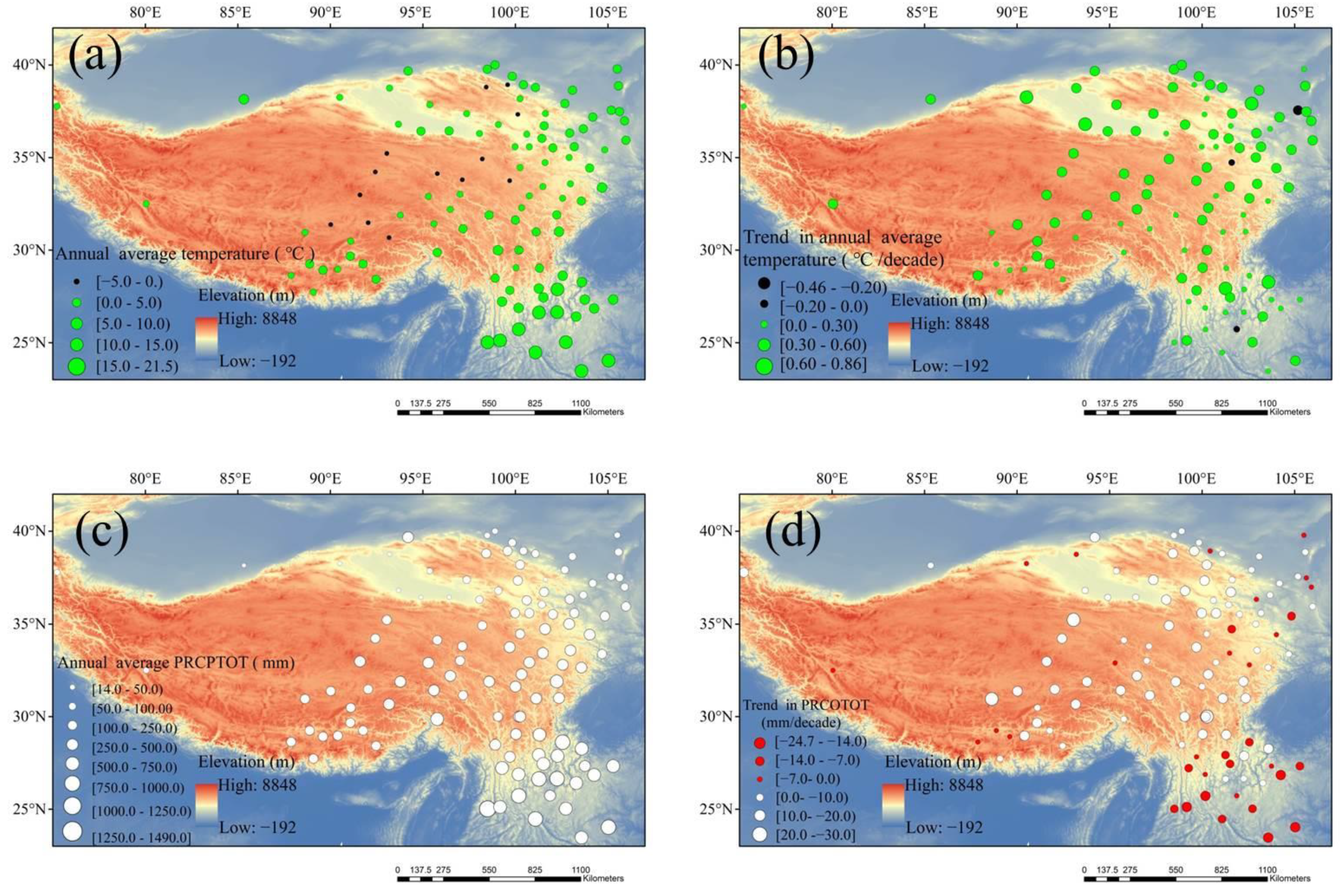
The annual average temperature in the study area exhibits spatial heterogeneity (Figure 2a). It decreases gradually from south to north and from the edges of the plateau to the interior. The spatial distribution of long-term (1970–2017) annual average temperature is shown in Figure 2b. Most of the stations showed a significant upward trend, except for three, which showed a downward trend. Note that the increase was slower in warmer areas and more rapid in cooler areas. The spatial distribution of long-term (1970–2017) precipitation (PRCPTOT) is shown in Figure 2c. Most of the stations showed significant increasing trends, although some stations in the southeast and on the edge of the plateau showed decreasing trends. The long-term precipitation exhibited spatial heterogeneity in the study area (Figure 2d), with a gradual decrease from southeast to northwest.
Figure 3 shows the multi-time-scale variation in the annual average temperature and annual total precipitation. The average temperature exhibited fluctuations and increased linearly from 1970 to 2017 (Figure 3a) at a rate of 0.33 °C/decade (slope: 0.033; R: 0.77). The annual total precipitation also showed fluctuations, with an overall increase (RR ≥ 1 mm) at a rate of 6.7 mm/decade (slope: 0.67; R: 0.3) (Figure 3g). However, the EEMD analysis revealed that all of the IMF components showed multiple fluctuations and clearly oscillated on different time scales.
The amplitudes of the IMF1 components of both the temperature and the PRCPTOT in 1970–1985 were smaller than those in 1986–2017, with variation periods of about 3.3 and 2.8 years, respectively (Figure 3b,h, respectively). The IMF2 component of the temperature had a significantly smaller amplitude in 1990–2010 than in the other periods, over a period of approximately 8.7 years (Figure 3c), whereas the IMF2 component of the PRCPTOT had a significantly smaller amplitude in 1990–2010 than in the other periods, over a period of approximately 6.4 years (Figure 3i). By contrast, the IMF3 component of temperature showed a significant increase in amplitude from the mid-to-late 1990s and then decreased in amplitude in the mid—to-late 2000s, over a period of approximately 13.7 years (Figure 3d). The IMF3 component of the PRCPTOT exhibited greater fluctuation and stronger periodicity than the IMF3 component of temperature, with a significant increase in amplitude starting in the 1990s (Figure 3j); the period was also 13.7 years. The IMF4 component of the temperature changed from the negative to the positive phase in 1994 and had an oscillation period of 48 years (Figure 3e). That of the PRCPTOT was generally in the negative phase from 1983 onward and became significantly smaller in amplitude from the 1990s onward; the oscillation period was 19.2 years (Figure 3k). The temperature and PRCPTOT trends may have reflected periodic oscillations on longer time scales, but they were not decomposed because of limitations in the length of the data. However, the temperature and PRCPTOT tended to increase with time (Figure 3f,l).
To compare the IMF components of the temperature and PRCPTOT and to reveal the essential oscillations of the original series, the variance contributions of the IMF were calculated (Table 2). The IMF1 component of the temperature accounted for 29.7% of the variance, which was the largest contribution, followed by the IMF2 (22.4%). That is, the interannual signal was the main component of the annual temperature variability in our study area. In addition, IMF3 and IMF4 showed periods of 13.7 and 48 years, respectively, on the interdecadal and multidecadal scales; together, they contribute 11.3% of the temperature variation. In addition, the overall trend accounted for 43.8% of the variation. The IMF1 component of the PRCPTOT accounted for 51.9% of the variance, followed by IMF4 (19.2%), IMF3 (15.8%), and IMF2 (9.6%). The interannual signal was also the main contributor to the PRCPTOT variability in our study area. By contrast, on the interdecadal and multidecadal scales, IMF3 and IMF4, with 13.7- and 19.2-year periods, respectively, contributed 19.1% of the PRCPTOT variability. However, the overall trend accounted for only 19.4% of the variance.
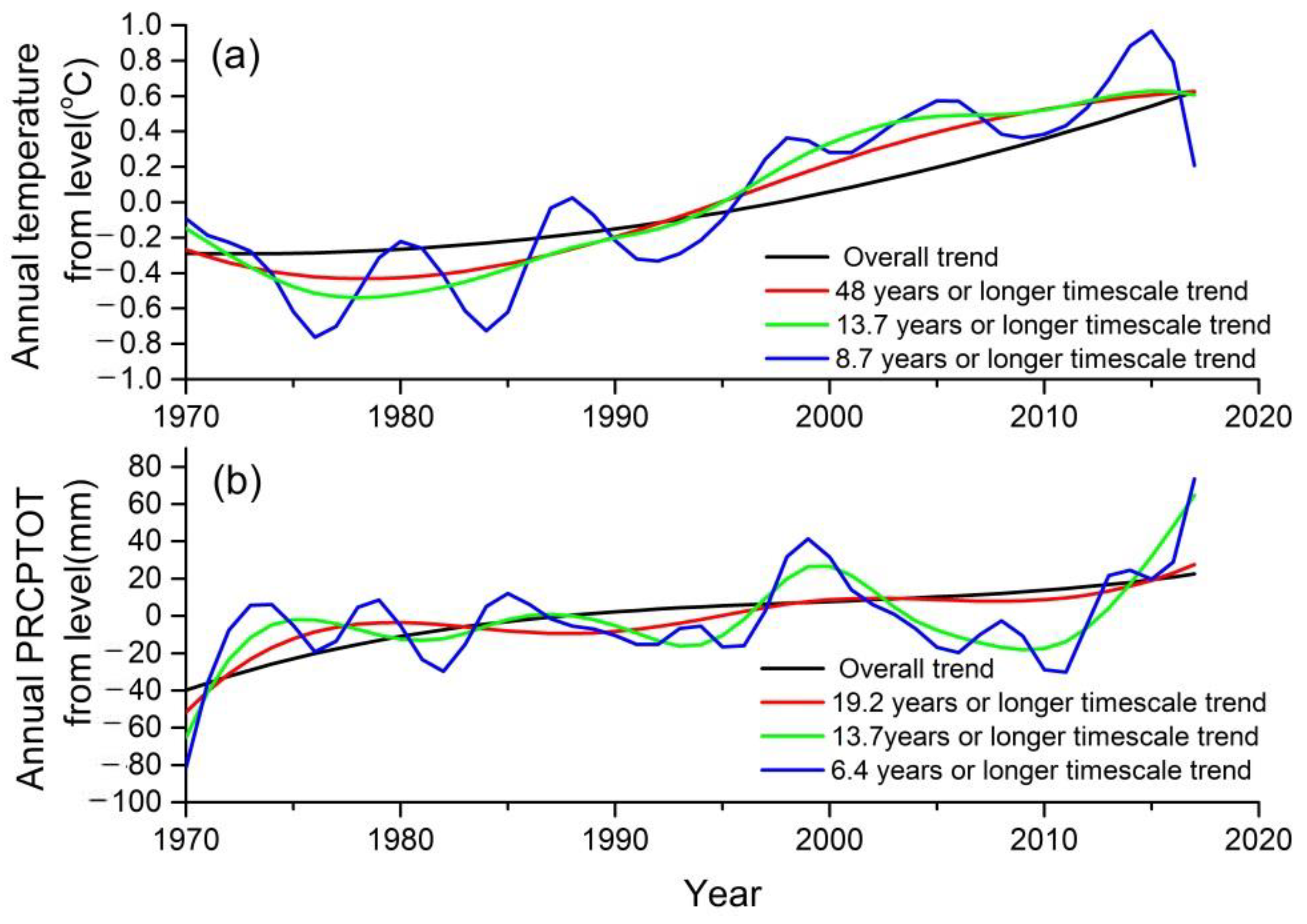
Figure 4 shows the oscillation period superimposed on the nonlinear variation. The temperature anomaly (Figure 4a) entered the positive phase in the mid-1990s. For the oscillation period of 8.7 years, below-average temperatures were recorded in 1970–1995, with three cooler and two warmer periods, and above-average temperatures were recorded after 1996, with three warmer periods and two cooler periods. Compared with that of the 8.7-year period, the oscillation amplitude of the 13.7- and 48-year periods was small. In addition, the overall trend of the PRCPTOT changed from negative to positive in the mid-1980s (Figure 4b). Over a period of 19.2 years, the PRCPTOT was below average from 1970 to 1997, and above average from 1998 onward; the oscillations were small in both cases. However, for the 13.7-year period, the PRCPTOT was also below average from 1970 to 1997, with two dry and wet periods. After 1998, the wet and dry periods clearly alternated, with a wet period from 1998 to 2004 and a dry period from 2005 to 2014. For the 6.4-year period, the PRCPTOT was below average overall from 1970 to 1997, but there were three wetter and three drier periods of variability. Thereafter, after a wet period in 1997–2004, there was a shift to a dry period in 2005–2012, with the PRCPTOT increasing again after 2012. In general, although both the temperature and precipitation showed an increasing trend, their oscillation periods differed significantly, indicating that the changes in temperature and precipitation were not completely synchronized.
The annual precipitation in our study area (PRCPTOT) was 505 mm. The average monthly precipitation as a percentage of the annual precipitation is shown in Figure 5. It can be seen that the monthly precipitation was unevenly distributed throughout the year.

3.2. Variation in Precipitation Extremes

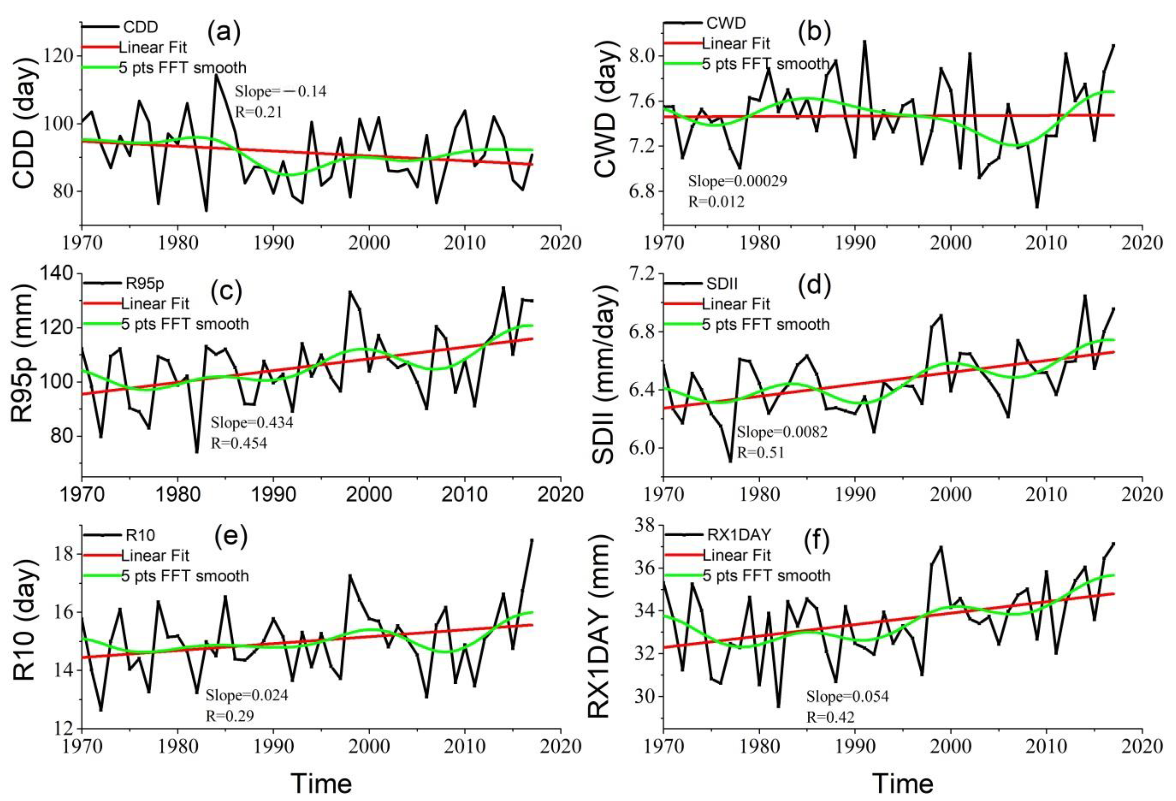
Figure 6 shows the annual precipitation extreme indices from 1970 to 2017. The numbers of consecutive dry days (CDD) and consecutive wet days (CWD) exhibited different trends from 1970 to 2017 (Figure 6a,b, respectively). The maximum and minimum values of CDD were 144.4 and 74.3 days, respectively. The average CDD was 91.4 days, with a decreasing trend of −1.4 days/10a. The maximum and minimum values of the CWD were 8.1 and 6.7 days, respectively. The average CWD was 7.5 days, and no clear trend appeared; the rate of increase was only 0.0029 days/10a. The CDD and CWD trends showed decreasing drought intensity and wetter conditions in the study area. The R95P, SDII, R10, and Rx1-day all showed increasing trends, with fluctuation from 1970 to 2017 (Figure 6c–f). The maximum and minimum R95p values were 134.7 and 74.2 mm, respectively. The average R95p was 105.7 days, with a rate of decrease of 4.34 mm/10a. The maximum and minimum SDII values were 7.0 and 5.9 mm/day, respectively. The average SDII was 6.5 days, with a rate of decrease of 0.08 mm/day/10a. The maximum and minimum Rx1-day values were 37.1 and 29.5 days, respectively. The average Rx1-day was 33.5 days, with a rate of decrease of 0.54 mm/10a. The maximum and minimum R10 values were 18.5 and 12.6 days, respectively. The average R10 was 15.0 days, with a rate of decrease of 0.24 day/10a.
To further analyze the nonlinear and periodic variation in the extreme-precipitation indices, an EEMD analysis was performed. The IMF components and oscillation periods of each index are shown in Table 3. The variance contribution of each IMF component was calculated and is also presented in Table 3. All the indices showed quasi-3-year and quasi-6-year interannual variability. The interannual variability was also a major component of each index (IMF1 and IMF2), accounting for 73.9% (CDD), 65.1% (CWD), 68.4% (R95p), 65% (SDII), 70.8% (R10), and 68.2% (Rx1day) of the variance. The quasi-3-year oscillation explains 40%–60% of the variance of each index. These results indicate that the extreme precipitation in the study area was dominated by interannual variability. On a multi-decade time scale, each index exhibited different characteristics. The CDD and R95p exhibited periodic oscillations of 13.7 and 24 years, and periodic oscillations of 13.7 and 19.2 years were found in the R10. The Rx1-day showed oscillations of 16 and 24 years on the interdecadal and multidecadal scales, respectively. The interdecadal periods of the CWD are 12 and 48 years, respectively, whereas the SDII exhibited interdecadal variations with periods of 19.2 and 48 years. Overall, the indices contributed 13.6% (CDD), 7% (CWD), 20.7% (R95p), 21.1% (SDII), 12.5% (R10), and 23% (Rx1-day) of the variance. Note that the 48-year period of the IMF4 components of the CWD and SDII may have been affected by the maximum length of the time series we used, as noted in the literature [62,63].
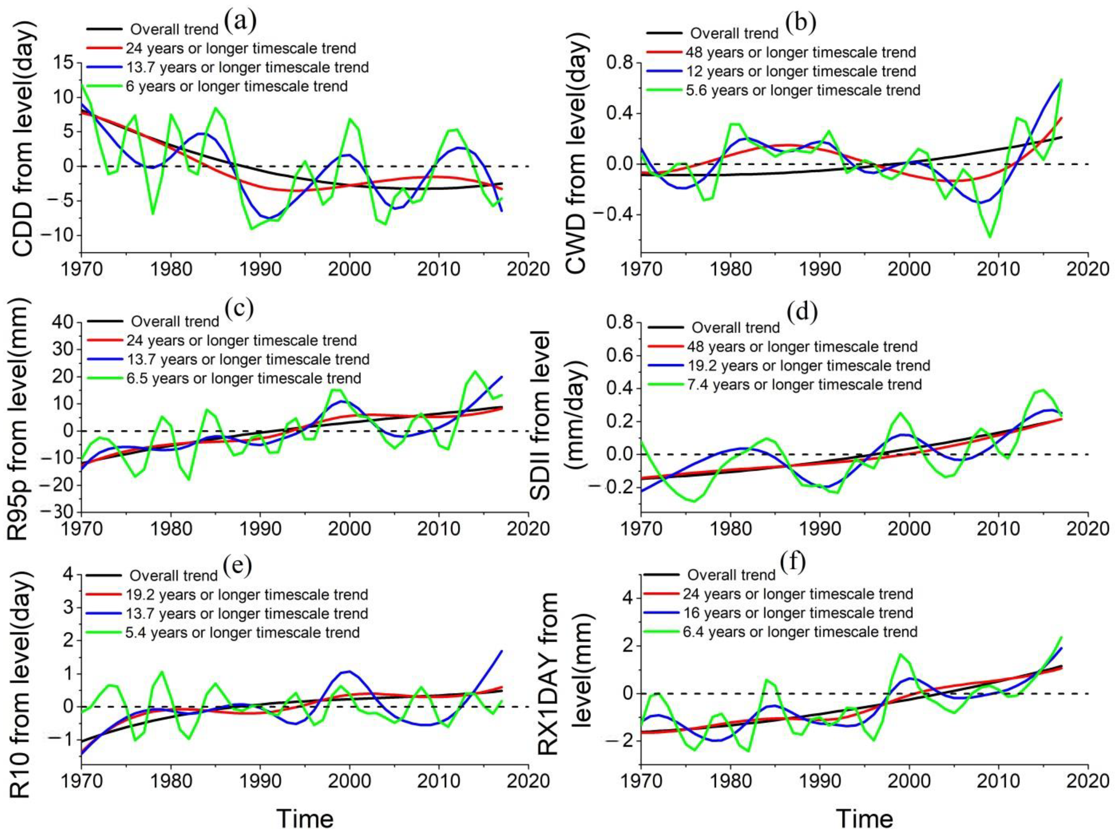
Figure 7 shows the oscillation period of each extreme-precipitation index superimposed on its nonlinear trend. The CDD anomaly (Figure 7a) entered the negative phase in the mid-to-late 1980s. For the oscillation period of 13.7 years, above-average CDD occurred in 1970–1987, with a dryer period and a wetter period, and below-average CDD occurred after 1987, with two dryer periods and two wetter periods. On the 6-year scale, the oscillation cycle was more volatile, whereas on the 24-year scale, it did not change significantly. The overall decreasing trend indicates a gradual decrease in consecutive dry days. By contrast, the fluctuations on these three scales (Figure 7b) show that the CWD was anomalously negative overall in the 1970s and anomalously positive from 1980 to the mid-1990s. It subsequently became negative and decreased gradually until the end of the 2000s, after which it showed a gradual upward trend. Overall, the trend was upward, indicating that the CWD increased. The changes in the CDD and CWD indicate that the climate in the study area is becoming wetter. The R95p and R10 showed very similar fluctuations on these three scales (Figure 7c,e, respectively); they were anomalously negative overall from 1970 to the mid-1990s, after which they become positive. From 2000 to 2010, they decreased gradually and became negative, after which they showed an upward trend and become positive. Overall, they showed a gradual increase; that is, the amount of extreme precipitation and the number of extreme-precipitation days increased, and the precipitation extremes were greater in the study area. However, the SDII was anomalously negative on these three scales from 1970 to the mid-1990s (Figure 7d), especially on the 7.4- and 19.2-year scales, with a dryer period (below zero) and a wetter period, and was anomalously positive overall thereafter. A dry period and wet period (above zero) occurred on the 19.2-year scale. Similarly, on these three scales, the Rx1-day was anomalously negative overall from 1970 to the late 1990s (Figure 7f), with two partially dry and partially wet periods (below zero) on the same 16-year scale; it was anomalously positive overall thereafter. Overall, the SDII and Rx1-day exhibited an upward trend, indicating that the maximum monthly single-day precipitation and the intensity of the single-day precipitation both increased. Overall, the climate in the study area gradually became warmer and wetter from 1970 to 2000, and the climate fluctuations became more pronounced after 2000, with precipitation and extreme precipitation experiencing a slowing increase.

3.3. Spatial Distribution and Trends of Extreme Precipitation

Figure 8 shows the spatial distribution of the extreme precipitation indices in our study region. The spatial distribution of the CDD (Figure 8a) indicates that the CDD was generally higher in the northern part of the plateau than in the southern part. The lowest CDD was found in the central plateau, and the highest CDD was near Qaidam Basin. The spatial pattern of the CWD showed the opposite distribution, as shown in Figure 8b; the CWD was generally higher in the southern part of the plateau than in the northern part. The lowest CWD appeared near Qaidam Basin. The spatial distribution of the R95p (Figure 8c) showed a gradual increase from north to south on the plateau. The lowest value appeared in the Qaidam Basin, and the highest value appeared on the Yunnan–Guizhou Plateau. The spatial distributions of SDII, R10, and Rx1-day (Figure 8d–f, respectively) were similar to that of R95p. The highest value appeared on the Yunnan–Guizhou Plateau, and the lowest value appeared in the Qaidam Basin. Therefore, Figure 8a–f suggests that precipitation is extremely low in the northern part of the plateau, whereas the southern part of the plateau, especially the Yunnan–Guizhou area, is relatively wet.
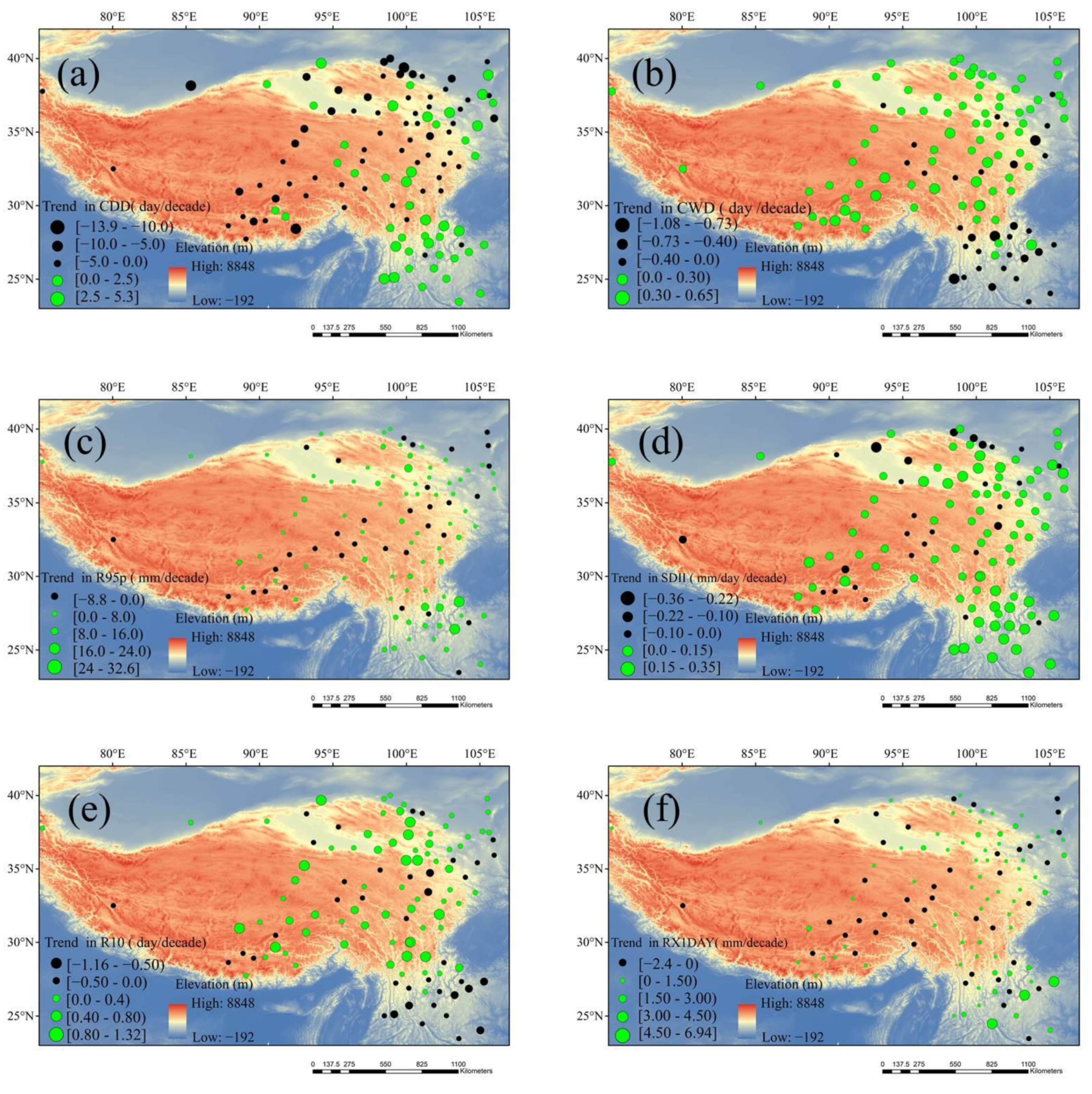
The spatial trend of each extreme precipitation index is shown in Figure 9. The CDD exhibited clear spatial heterogeneity (Figure 9a). Overall, most of the stations showed clear changes from 1970 to 2017. The trend was mainly downward on the Qinghai–TP and mainly upward on the Yunnan–Guizhou Plateau. By contrast, the CWD showed the opposite trend in spatial distribution (Figure 9b): primarily upward and downward trends on the TP and Yunnan–Guizhou Plateau, respectively. The overall trend for the R95p (Figure 9c) was upward, although some stations, mainly in the southeastern part of the plateau, showed decreases. Most of the stations showed increases in SDII; only 28 stations scattered across the TP showed overall decreases (Figure 9d). The R10 decreased significantly on the Yunnan–Guizhou Plateau, and most of the stations on the TP showed significant increases (Figure 9e). The Rx1-day increased significantly in much of the study area (Figure 9f), although some of the stations across the study area showed decreases. Overall, most of the stations showed significant changes in the extreme-precipitation indices, with clear differences in spatial distribution. These results also indicate spatial heterogeneity and diversity in extreme precipitation in mountainous areas (plateaus).

3.4. Spatiotemporal Pattern of Extreme Precipitation

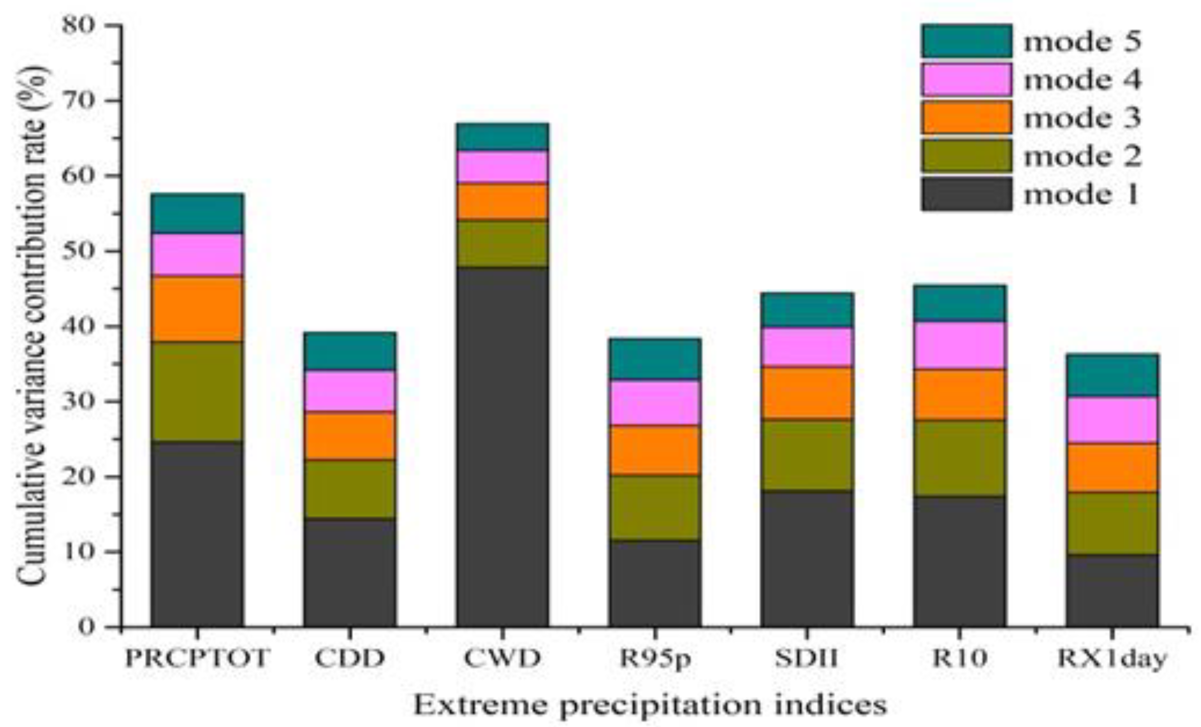
The empirical orthogonal function (EOF) was used to analyze the spatial and temporal patterns of extreme precipitation. North’s method [64] was used to test the number of significant orthogonal functions. Figure 10 shows the cumulative variance of the first five EOF eigenvectors of the extreme-precipitation indices. The first five EOFs account for 38.4–66.9% of the total variance. The variance of some of these indices does not make a large contribution to the total, indicating that the extreme-precipitation pattern in the study area is complex. The first two EOFs of each index were selected for analysis. These EOFs and their corresponding principal components therefore also reflect the spatial and temporal structure of the extreme precipitation to some degree.
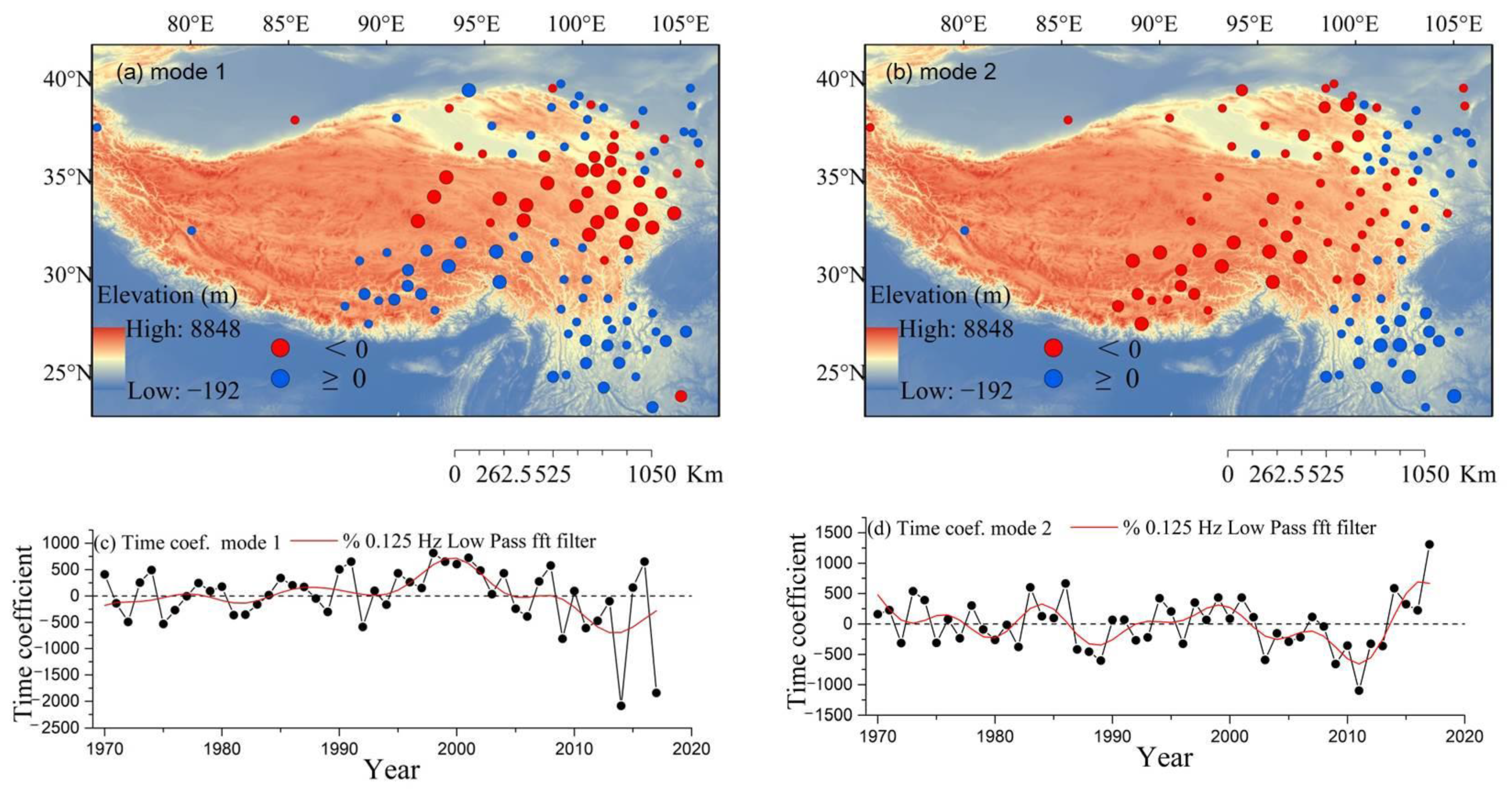
The spatial patterns of modes 1 and 2 of the PRCPTOT accounted for 24.4% and 13.3% of the total variance, respectively; moreover, these two spatial modes passed the North test [64] (Figure 11). EOF mode 1 clearly showed an anti-phase distribution pattern, with higher PRCPTOT in the southern and northern parts of the plateau and lower PRCPTOT in the central part (Figure 11a). The time coefficient of EOF mode 1 exhibited fluctuations characterized by interannual and intergenerational variation. In addition, it showed a weak upward trend before 2000 and a clear downward trend after 2000 (Figure 11c). This result indicates that EOF mode 1 of the PRCPTOT decreased after 2000. However, EOF mode 2 clearly showed an anti-phase-distribution pattern, with higher and lower PRCPTOT east and west of longitude 100°E, respectively (Figure 11b). The time coefficient of EOF mode 2 also showed interannual and intergenerational variation; it fluctuated before 2000, decreased from 2000 to 2010, and increased significantly after 2010 (Figure 11d). These results indicates that EOF mode 2 of the PRCPTOT began to strengthen in 2000.
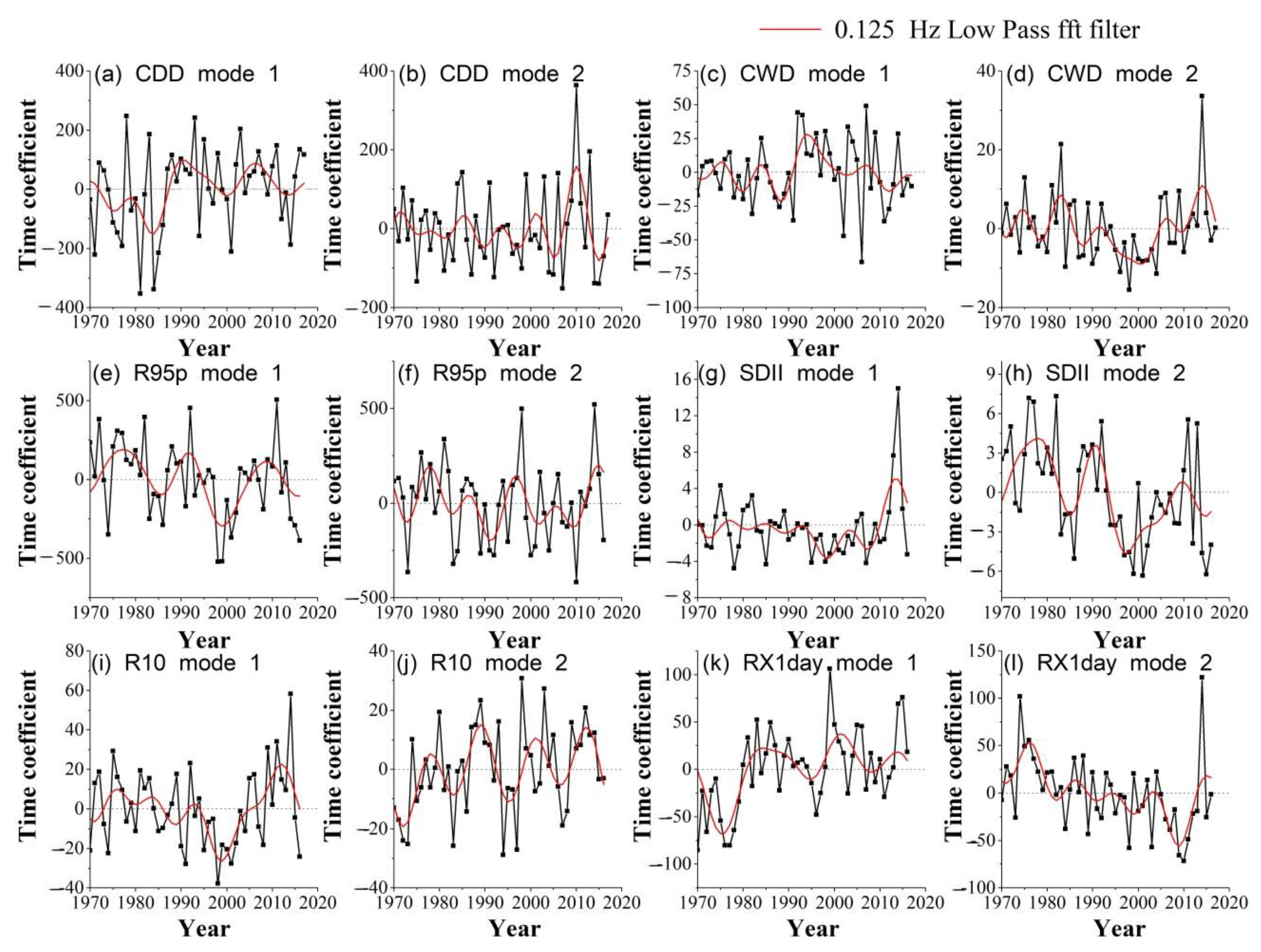
The spatial patterns of EOF modes 1 and 2 of the CDD accounted for 14.4% and 7.8% of the total variance, respectively, and passed the North test. They showed a consistent pattern, in which mode 1 exhibited the opposite behavior to mode 2, and they showed negative and positive values overall (Figure 12a,b). The time coefficients of EOF modes 1 and 2 indicate that they were characterized by interannual and intergenerational variation (Figure 13a,b). However, EOF modes 1 and 2 of the CWD accounted for 47.8% and 6.3% of the total spatial variance, respectively, and passed the North test. EOF mode 1 of CWD showed alternating positive and negative values, with no clear regional differences (Figure 12c). The time coefficient of EOF mode 1 showed a clear downward trend after the mid-1990s (Figure 13c). This result indicates that EOF mode 1 of the CWD decreased after the mid-1990s. However, EOF mode 2 showed an anti-phase distribution pattern; it was positive and negative north and south of approximately 32°N, respectively (Figure 12d). The time coefficient of EOF mode 2 of the CWD increased significantly after 2000 (Figure 13d), indicating that this mode began to strengthen in 2000.
The spatial patterns of EOF modes 1 and 2 of the R95p accounted for 11.6% and 8.6% of the total variance, respectively, and passed the North test. EOF mode 1 showed an anti-phase distribution pattern, where it was negative and positive in the southwestern and northeastern parts of the plateau, respectively (Figure 12e). However, EOF mode 2 of the R95p showed alternating positive and negative values, with no clear regional differences (Figure 12f). The time coefficients of modes 1 and 2 were characterized by interannual and intergenerational variation (Figure 13e,f), indicating periodic changes.
The spatial patterns of modes 1 and 2 of SDII accounted for 18.1% and 9.5% of the total variance, respectively, and passed the North test. For mode 1, the negative values were mainly concentrated in the southern part of the TP, and positive values appeared in the central part (Figure 12g). However, for mode 2, the negative values were mainly concentrated in the southeastern part of the study area (Figure 12h). The time coefficient of EOF modes 1 and 2 fluctuated with an upward trend after 2000 (Figure 13g,h), indicating that they began to strengthen after 2000.
The spatial patterns of EOF modes 1 and 2 of the R10 accounted for 17.4% and 10.2% of the total variance, respectively, and passed the North test. For mode 1, the negative and positive values were mainly concentrated south and north of approximately 32°N, respectively (Figure 12i). However, for mode 2, the negative values were mainly concentrated in the southeastern and northeastern parts of the study area (Figure 12j). The time coefficients of EOF modes 1 and 2 of the R10 are shown in Figure 12i and Figure 12j, respectively. That of mode 1 showed a clear downward trend from 1970 to 2000 and increased significantly after 2000 (Figure 13i), indicating that this mode was weak from 1970 to 2000 and became stronger thereafter. However, the time coefficient of mode 2 showed fluctuations with an upward trend (Figure 13j), indicating volatility with overall strengthening after the 1970s.
The spatial patterns of EOF modes 1 and 2 of the Rx1-day accounted for 9.6% and 8.3% of the total variance, respectively, and passed the North test. For EOF mode 1, the negative and positive values were mainly concentrated in the southeastern and northwestern parts of the plateau, respectively (Figure 12k). By contrast, for mode 2, the negative values are concentrated mainly in the southwestern part of the study area, and the positive values are concentrated mainly in the northeastern and southwestern parts of the plateau (Figure 12l). The time coefficient of EOF mode 1 of the Rx1-day showed fluctuations with an upward trend, indicating overall strengthening, and that of EOF mode 2 showed fluctuations with a downward trend, indicating overall weakening (Figure 13k,l). Overall, the spatiotemporal patterns of EOF modes 1 and 2 of each extreme-precipitation index showed significant differences and were not uniform, suggesting that the extreme precipitation in the study area exhibited complex spatiotemporal patterns.

3.5. Correlation between Extreme Precipitation Indices and Their Association with Ocean-Oscillation Factors

Most precipitation indices are related to annual precipitation (PRCPTOT), which is strongly correlated with extreme precipitation [65,66]. To further analyze whether the extreme-precipitation indices selected in our study reflected the annual precipitation and to explore the correlation between the extreme-precipitation indices, the Spearman’s correlation coefficient was calculated.
Table 4 shows the correlations between the extreme-precipitation indices and the PRCPTOT. The Spearman correlation coefficients between the PRCPTOT and R10 exceeded 0.9, and those between the PRCPTOT and R95p, SDII, and Rx1-day exceeded 0.6 (p < 0.01). However, although the PRCPTOT was positively correlated with CWD, with a correlation coefficient of 0.2, and negatively correlated with CDD, with a correlation coefficient of −0.2, neither result was statistically significant.
Therefore, the indices selected in our study (R95p, SDII, R10, and Rx1day) reflect the variation in annual precipitation. The Spearman correlation coefficients between the PRCPTOT (and other indicators), CDD, and CWD were not high. These results indicate that the factors affecting the CDD and CWD were complex in the highland and mountainous areas. In addition, Table 4 shows that there was a statistically significant correlation between the precipitation indices. Overall, the timing of the extreme-precipitation events in the highlands was consistent, with increased total precipitation and increased frequency, intensity, and values of extreme precipitation; the PRCPTOT was most strongly correlated with the R10 and R95p.
To examine the relationship between the extreme-precipitation events and the SST indices, the correlation coefficients between the extreme precipitation in the study area and the various SST indices for the Pacific and Indian oceans during 1970–2017 were calculated, as shown in Table 5. The TIOD was negatively correlated with the PRCPTOT, R95p, SDII, R10, and Rx1-day, but the correlation was significant (p < 0.05) only for the PRCPTOT, with a correlation coefficient of −0.29. It was positively correlated with the CDD and CWD, but the correlations were not statistically significant. The IOBW and CDD were negatively correlated, with a correlation coefficient of −0.34 (p < 0.05), but they were positively correlated with other extreme-precipitation indices; specifically, the relationships with the R95p, SDII, and Rx1day were statistically significant (p < 0.01 or p < 0.05), with correlation coefficients of 0.31, 0.42, and 0.29, respectively. In addition to the negative correlation between the IOWPS and CDD, the IOWPS was positively correlated with other extreme-precipitation indices; significant correlations were found with the CDD (correlation coefficient: −0.36), R95p (0.34), SDII (0.43), and Rx1day (0.32). The PDO and CDD were negatively correlated, with a correlation coefficient of 0.31 (p < 0.05); they were positively correlated with other extreme-precipitation indices, but the correlations were not statistically significant. By contrast, strong positive correlations appeared between the WPWPS and PRCPTOT, R95p, SDII, R10, and Rx1day, with correlation coefficients of 0.40, 0.48, 0.57, 0.38, and 0.48, respectively; all of these correlations were statistically significant. However, the ENSOM was negatively correlated with all the precipitation indices, although the correlation was significant (p < 0.01 or p < 0.05) only for the R95p and Rx1day, with correlation coefficients of −0.29 and −0.4, respectively. By contrast, the SO was positively correlated with all the extreme-precipitation indices, but the correlation was significant only for the CDD and Rx1day (p < 0.05), with correlation coefficients of 0.35 and 0.33, respectively. Note that the correlation coefficients between the SIOD and each extreme-precipitation index were small, and none were statistically significant. These findings suggest that the IOWPS and WPWPS were the most important SST indices affecting the study area. These results also show that the SST anomalies in the Pacific and Indian oceans affected the precipitation and extreme precipitation in the study area.
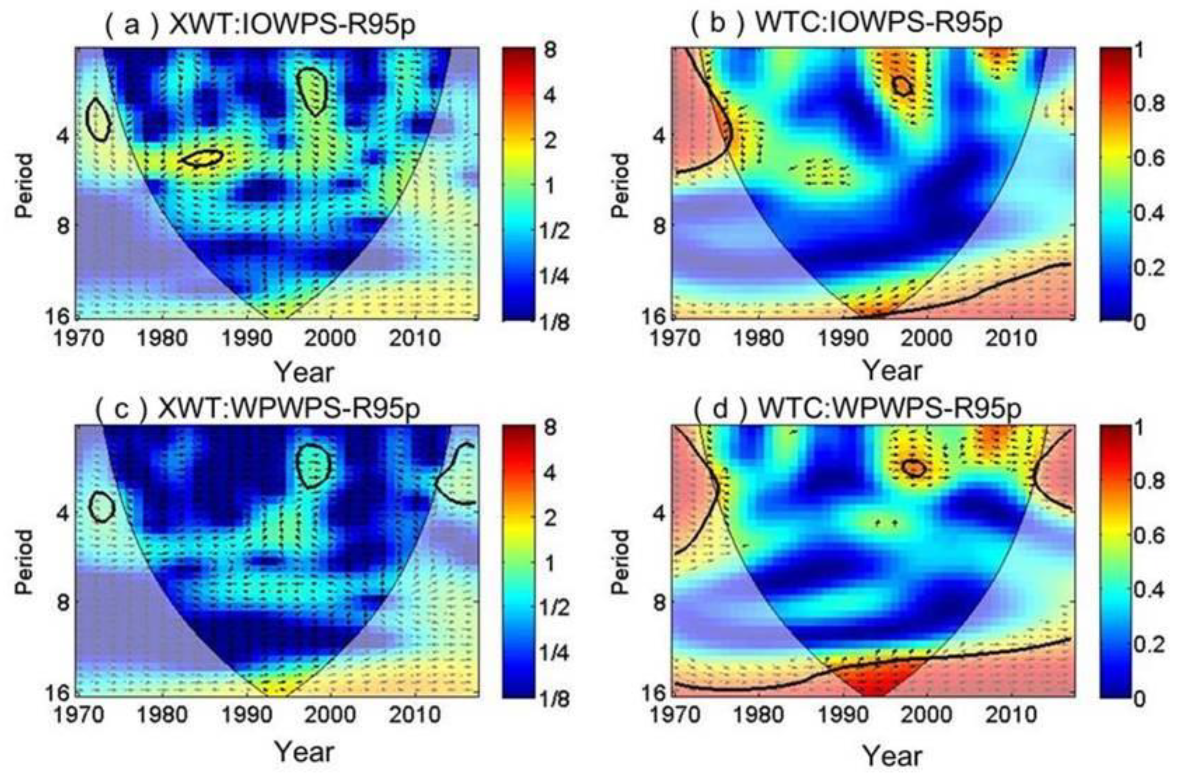
To further explore the relationship between the SST indices and the precipitation and extreme precipitation in the study area, an EEMD analysis was performed. The IMF components of the SST indices are presented in Table 6. The IMF1 component for each SST index oscillated over a 3-year period; the IMF2 component showed periodic oscillation over a period of 6–10 years, and the IMF3 component shows periodic oscillation over a period of 13–19 years. On the basis of Table 4 and Table 5, we selected the extreme-precipitation index, R95p and the SST indices, IOWP and WPWPS, to further analyze the association between extreme precipitation and SST.
The relationship between the SST indices (IOWP and WPWPS) and extreme precipitation events (R95p) in terms of duration and frequency was determined using continuous wavelet transform (CWT), and the relationships of the IOWP and WPWPS with R95p were investigated using the XWT. Next, the wavelet-transform coherence (WTC) between the two CWTs was used to determine the statistical coherence and confidence in the noise control. The results are shown in Figure 14. The XWT correlation between the IOWP and R95p revealed three significant power bands: a 3–4-year period from 1970 to 1980 (band (1)), a 6–7-year period from 1980 to 1990 (band (2)), and another from approximately 1990 to 2020 (band (3)) at low frequencies. The arrows indicating bands 1 and 2 are very similar and indicate that the two time series were in a positive phase, with a phase difference of 135°. However, the arrow for the third band indicates that the two time series were in a negative phase, with a phase difference of approximately 270° (Figure 14a). The WTC between the IOWP and R95p showed a 2–3-year period around 1990–2000 (Figure 14b), during which the two time series were in a positive phase, with a phase difference of approximately 90°.

4. Discussion

The TPS may be one of the most sensitive regions to current global climate change. There is evidence that climate warming began earlier (early 1950s) in this region than in the Northern Hemisphere (mid-1970s). In addition, extreme precipitation on the TP has reportedly increased in recent years [66,67,68,69,70,71].
These increases have shown large regional differences; annual precipitation fluctuations are slowly increasing in the large central and western regions. The eastern part of the plateau varies from north to south between areas of rapidly intensifying and rapidly weakening precipitation. The intensity and frequency of extreme-precipitation events show similar variation patterns [69]. We found that the temperature on the TPS showed an upward trend, which was more pronounced in the regions with low temperatures than in the regions with high temperatures. In addition, the precipitation and extreme precipitation showed an upward trend. The total extreme precipitation, number of extreme precipitation days, maximum single-day precipitation, and extreme single-day precipitation intensity all showed increasing trends, and each extreme-precipitation index oscillated at different time scales. The extreme-precipitation indices generally showed periods of 3 years, 5–7 years, 2–15 years, 19–24 years, and longer. The quasi-3-year periodic oscillation made the largest contribution to the extreme precipitation, and the extreme-precipitation indices were closely related to each other. These results were similar to those of Feng et al. [72]. Cao et al. [71] noted that summer extreme precipitation in the east–central part of the plateau is generally increasing, except for a decreasing trend in eastern Tibet. In addition, Zhao et al. [68] showed that the amount and frequency of intense summer precipitation on the eastern TP decreased from southeast to northwest, whereas the precipitation intensity increased gradually from south to north. The annual precipitation has increased over most of the TP, as has instability. By contrast, our study found that the PRCPTOT decreased gradually from southeast to northwest; in the northern part of the plateau, rainfall is extremely scarce, and the southern part, especially the Yunnan–Guizhou area, is relatively wet. The spatial distributions of the R95p, SDII, R10, and Rx1-day showed gradual increases from north to south on the plateau. The extreme-precipitation indices at most of the stations showed clear trends, but the spatial distributions clearly varied because of the notable surface heterogeneity of highlands and mountains. Moreover, the EOF analysis showed certain regularities in the spatial patterns of the precipitation and extreme precipitation in the study area, and EOF modes 1 and 2 of each extreme-precipitation index exhibited clear differences, indicating that extreme precipitation is characterized by local clustering. This discrepancy may be attributed to the fact that Zhao et al.’s [68] study focuses on the variability of summer extreme precipitation, whereas our study considers annual-scale precipitation and extreme precipitation. In addition, there are significant seasonal differences in precipitation in the study area, and thus extreme precipitation is not spatially uniform. By contrast, precipitation exhibits complex spatial behavior owing to differences in surface topography [73,74] and the topographic enhancement of precipitation [75]. Precipitation and precipitation variability on the TP are correlated with elevation [76,77], and precipitation and extreme precipitation on the TP vary with elevation [77,78]. These variations produce the complex spatial distribution of extreme precipitation.
The effects of atmospheric circulation on precipitation and extreme precipitation on the TP have been reported [52,72,79]. Increased Indian Ocean SST will increase the Eurasian temperature meridional gradient and thus strengthen the Middle East Jet [80], which can significantly affect the climate in southern Asia and strengthen the trough in the southern TP, further enhancing water-vapor transport from western Asia and the Bay of Bengal to China [81]. The IOD is significantly correlated with flood precipitation on the TP [82]. The Pacific SST anomaly also affects extreme precipitation on the TP [52]. To analyze the effects of SST anomalies on precipitation and extreme precipitation on the TP, four indices (TIOD, IOBW, SIOD, and IOWPS) indicating SST anomalies in the Indian Ocean and four indices (PDO, WPWPS, ENSOM, and SOI) indicating SST anomalies in the Pacific Ocean were selected for analysis. Differences in the Pearson correlation coefficients between the eight SST indices and each extreme-precipitation index in the study area were found. Among them, the IOWPS and WPWPS were the most strongly correlated with each extreme-precipitation index. Further analysis of each SST index by the EEMD method revealed oscillation periods on different scales (3, 6–10, and 13–19 years). These oscillation periods were similar to those of the extreme-precipitation indices in the study area (3, 5–7, 12–15, and 19–24 years). Moreover, the CWT analysis of the relationships of the IOWPS and WPWPS with the R95p confirmed this result, although the periods were not completely synchronized. The timings of the extreme-precipitation events generally lagged behind those of the SST anomalies. These results indicate that ocean-anomaly signals can be transmitted or stored by complex ocean dynamics and thermal processes, as well as tropical SST anomalies influencing regional climate changes through atmospheric bridging effects [81,83,84,85]. Further in-depth studies are needed on the mechanism of the effect of SST anomalies in the Pacific and Indian oceans on extreme precipitation in the study area.

5. Conclusions

To study the trends, patterns, and relationship with the oceanic oscillation factors of extreme precipitation on the Tibetan Plateau and its surrounding areas, the observation data of 113 meteorological stations from 1971 to 2017 were used. The main findings were as follows:
(1) Precipitation and extreme precipitation do not exhibit simple linear increases with increasing temperature. The total extreme precipitation, number of extreme-precipitation days, maximum single-day precipitation, and extreme single-day precipitation intensity all showed fluctuations with an overall increase. The quasi-3-year oscillation made the largest contribution to the extreme precipitation, the climate gradually became warmer and wetter from 1970 to 2000, and the climate fluctuations became more pronounced after 2000, with precipitation and extreme precipitation exhibiting a decelerating increase.
(2) The R95p, SDII, R10, and Rx1day increased gradually from north to south on the plateau. Most of the stations experienced significant variation in the extreme precipitation indices, and the spatial distributions showed clear differences. The extreme precipitation in the mountainous areas showed spatial heterogeneity and diversity.
(3) The spatiotemporal patterns of EOF modes 1 and 2 of each extreme-precipitation index showed significant differences and were not spatiotemporally uniform, but showed local clustering.
(4) The SST-index oscillation periods are similar to those of the extreme precipitation indices in the study area (3, 5–7, 12–15, and 19–24 years). The IOWPS and WPWPS were most strongly correlated with the extreme-precipitation indices, and the timings of the extreme-precipitation events lagged behind those of the SST anomalies.

Author Contributions

Conceptualization, W.H. and J.Y.; writing—original draft preparation, W.H., L.C. and J.S.; writing—review and editing, Q.H.; funding acquisition, W.H. and J.Y.; methodology, J.C. All authors have read and agreed to the published version of the manuscript.

Funding

This work was funded by the National Natural Science Foundation of China (42171038), the National Key Research and Development Program of China (2019YFC1510501), the Second Tibetan Plateau Scientific Expedition and Research Program (2019QZKK010206), the China Postdoctoral Science Foundation (2019M653905XB), the Central Asia Atmospheric Science Research Fund [(CAAS201703), and the Provincial Nature Science Research Project of Anhui Colleges (KJ2021A0670).

Data Availability Statement

Data are available upon reasonable request to the corresponding author.

Acknowledgments

We are grateful to the reviewers and for their valuable comments on this manuscript, We also thank the editor for his contribution to the manuscript.

Conflicts of Interest

The authors declare no conflict of interest.

References

  1. Stocker, T. (Ed.) Climate Change 2013: The Physical Science Basis. Contribution of Working Group I to the Fifth Assessment Report of the Intergovernmental Panel on Climate Change; Cambridge University Press: Cambridge, UK; New York, NY, USA, 2013; p. 1535. [Google Scholar]
  2. Meehl, G.A.; Arblaster, J.M.; Branstator, G. Mechanisms contributing to the warming hole and the consequent U.S. East–West differential of heat extremes. J. Clim. 2012, 25, 6394–6408. [Google Scholar] [CrossRef]
  3. Diaz, H.F.; Bradley, R.S. Temperature variations during the last century at high elevation sites. Clim. Chang. 1997, 36, 253–279. [Google Scholar] [CrossRef]
  4. Diaz, H.F.; Eischeid, J.K. Disappearing “alpine tundra” Köppen climatic type in the western United States. Geophys. Res. Lett. 2007, 34, L18707. [Google Scholar] [CrossRef]
  5. Wang, Q.; Fan, X.; Wang, M. Recent warming amplification over high elevation regions across the globe. Clim. Dyn. 2013, 43, 87–101. [Google Scholar]
  6. Field, C.B.; Barros, V.; Stocker, T.F.; Dahe, Q. (Eds.) Managing the Risks of Extreme Events and Disasters to Advance Climate Chang. Adaptation; Cambridge University Press: Cambridge, UK, 2012; p. 582. [Google Scholar]
  7. Easterling, D.R. Climate extremes: Observations, modeling, and impacts. Science 2000, 289, 2068–2074. [Google Scholar] [CrossRef]
  8. Mishra, A.; Liu, S.C. Changes in precipitation pattern and risk of drought over India in the context of global warming. J. Geophys. Res. Atmos. 2014, 119, 7833–7841. [Google Scholar] [CrossRef]
  9. Donat, M.G.; Lowry, A.L.; Alexander, L.V.; O’Gorman, P.A.; Maher, N. More extreme precipitation in the world’s dry and wet regions. Nat. Clim. Chang. 2016, 6, 508–513. [Google Scholar] [CrossRef]
  10. Lehmann, J.; Coumou, D.; Frieler, K. Increased record-breaking precipitation events under global warming. Clim. Chang. 2015, 132, 501–515. [Google Scholar] [CrossRef]
  11. Pachauri, R.K.; Meyer, L.A. (Eds.) Climate Change 2014: Synthesis Report, Contribution of Working Groups I, II and III to the Fifth Assessment Report of the Intergovernmental Panel on Climate Change; IPCC: Geneva, Switzerland, 2014; p. 151. [Google Scholar]
  12. Trenberth, K.E. Observations: Surface and Atmospheric Climate Change, in Climate Change 2007: The Physical Science Basis. Contribution of Working Group I to the Fourth Assessment Report of the Intergovernmental Panel on Climate Change; Solomon, S., Qin, D., Manning, M., Chen, Z., Marquis, M., Averyt, K.B., Tignor, M., Miller, H.L., Eds.; Cambridge University Press: New York, NY, USA, 2007; pp. 235–336. [Google Scholar]
  13. Trenberth, K.E. Changes in precipitation with climate change. Clim. Res. 2011, 47, 123–138. [Google Scholar] [CrossRef]
  14. Zhang, X.; Zwiers, F.W.; Hegerl, G.C.; Lambert, F.H.; Gillett, N.P.; Solomon, S.; Stott, P.A.; Nozawa, T. Detection of human influence on twentieth-century precipitation trends. Nature 2007, 448, 461–465. [Google Scholar] [CrossRef] [PubMed]
  15. Lau, K.M.; Wu, H.T. Detecting trends in tropical rainfall characteristics. Int. J. Climatol. 2008, 27, 979–988. [Google Scholar] [CrossRef]
  16. O’Gorman, P.A.; Paul, A. Sensitivity of tropical precipitation extremes to climate change. Nat. Geosci. 2012, 5, 697–700. [Google Scholar] [CrossRef]
  17. Villarini, G.; Smith, J.A.; Vecchi, G.A. Changing frequency of heavy rainfall over the Central United States. J. Clim. 2013, 26, 351–357. [Google Scholar] [CrossRef]
  18. Alexander, L.V.; Zhang, X.B.; Peterson, T.C.; Caesar, J.; Vazquez-Aguirre, J.L. Global observed changes in daily climate extremes of temperature and precipitation. J. Geophys. Res. 2006, 111, D05109. [Google Scholar] [CrossRef]
  19. Min, S.K.; Zhang, X.; Zwiers, F.W.; Hegerl, G.C. Human contribution to more intense precipitation extremes. Nature 2011, 470, 378–381. [Google Scholar] [CrossRef]
  20. Westra, S.; Alexander, L.V.; Zwiers, F.W. Global increasing trends in annual maximum daily precipitation. J. Clim. 2013, 26, 3904–3918. [Google Scholar] [CrossRef]
  21. Peterson, T.C.; Zhang, X.; Brunet-India, M.; Vázquez-Aguirre, J.L. Changes in North American extremes derived from daily weather data. J. Geophys. Res. Atmos. 2008, 113, D07113. [Google Scholar] [CrossRef]
  22. Aguilar, E.; Barry, A.A.; Brunet, M.; Ekang, L.; Fernandes, A.; Massoukina, M.; Mbah, J.; Mhanda, A.; Nascimento, D.J.; Peterson, T.C.; et al. Changes in temperature and precipitation extremes in western central Africa, Guinea Conakry, and Zimbabwe, 1955–2006. J. Geophys. Res. 2009, 114, D02115. [Google Scholar] [CrossRef]
  23. Zhai, P.; Sun, A.; Ren, F.; Liu, X.; Zhang, G.Q. Changes of climate extremes in china. Clim. Chang. 1999, 42, 203–218. [Google Scholar] [CrossRef]
  24. Zhai, P.; Zhang, X.; Hui, W.; Pan, X. Trends in total precipitation and frequency of daily precipitation extremes over china. J. Clim. 2005, 18, 1096–1108. [Google Scholar] [CrossRef]
  25. Yao, J.; Chen, Y.; Guan, X.; Zhao, Y.; Chen, J.; Mao, W. Recent climate and hydrological changes in a mountain-basin system in xinjiang, China. Earth-Sci. Rev. 2022, 226, 103957. [Google Scholar] [CrossRef]
  26. Feng, L.; Zhou, T.; Wu, B.; Tim, L.I. Projection of future precipitation change over China with a high-resolution global atmospheric model. Adv. Atmos. Sci. 2011, 28, 464–476. [Google Scholar] [CrossRef]
  27. Fu, G.; Yu, J.; Yu, X.; Ouyang, R.; Zhang, Y.; Ping, W.; Liu, W.; Min, L. Temporal variation of extreme rainfall events in China, 1961–2009. J. Hydrol. 2013, 487, 48–59. [Google Scholar] [CrossRef]
  28. Wang, Y.; Zhou, L. Observed trends in extreme precipitation events in China during 1961–2001 and the associated changes in large-scale circulation. Geophys. Res. Lett. 2005, 32, 982–993. [Google Scholar] [CrossRef]
  29. Yu, R.; Li, J. Hourly rainfall changes in response to surface air temperature over eastern contiguous China. J. Clim. 2012, 25, 6851–6861. [Google Scholar] [CrossRef]
  30. Beniston, M.; Diaz, H.; Bradley, R. Climatic change at high elevation sites: An overview. Clim. Chang. 1997, 36, 233–251. [Google Scholar] [CrossRef]
  31. Rangwala, I.; Miller, J.; Xu, M. Warming in the Tibetan Plateau: Possible influences of the changes in surface water vapor. Geophys. Res. Lett. 2009, 36, L06703. [Google Scholar] [CrossRef]
  32. Liu, X.; Cheng, Z.; Yan, L.; Yin, Z. Elevation dependency of recent and future minimum surface air temperature trends in the Tibetan Plateau and its surroundings. Glob. Planet. Chang. 2009, 68, 164–174. [Google Scholar] [CrossRef]
  33. Qin, J.; Yang, K.; Liang, S.; Guo, X. The altitudinal dependence of recent rapid warming over the Tibetan Plateau. Clim. Chang. 2009, 97, 321–327. [Google Scholar] [CrossRef]
  34. Pederson, G.T.; Graumlich, L.J.; Fagre, D.B.; Kipfer, T.; Muhlfeld, C.C. A century of climate and ecosystem change in Western Montana: What do temperature trends portend? Clim. Chang. 2010, 98, 133–154. [Google Scholar] [CrossRef]
  35. Ives, J. Mountains of the world: A global priority. Mt. Res. Dev. 1997, 17, 375–376. [Google Scholar]
  36. Tennant, C.J.; Crosby, B.T.; Godsey, S.E. Elevation-dependent responses of streamflow to climate warming. Hydrol. Process. 2015, 29, 991–1001. [Google Scholar] [CrossRef]
  37. Johnston, V.E.; Borsato, A.; Frisia, S.; Spötl, C.; Dublyansky, Y.; Töchterle, P.; Hellstrom, J.C.; Bajo, P.; Edwards, R.L.; Cheng, H. Evidence of the rmosphilisation and elevation-dependent warming during the Last Interglacial in the Italian Alps. Sci. Rep. 2018, 8, 2680–2690. [Google Scholar] [CrossRef]
  38. Song, F.; Maocang, T. New evidence for the Qinghai-Xizang (Tibet) Plateau as a pilot region of climatic fluctuation in China. Chin. Sci. Bull. 1998, 43, 1745–1749. [Google Scholar]
  39. Cheng, G.; Wu, T. Responses of permafrost to climate change and their environmental significance, Qinghai-TibetPlateau. J. Geophys. Res. 2007, 112, F02S03. [Google Scholar]
  40. Liu, J.; Wang, S.Y.; Zhang, L. Climate warming and growth of high-elevation inland lakes on theTibetan Plateau. Glob. Planet. Chang. 2009, 67, 209–217. [Google Scholar] [CrossRef]
  41. Su, Z.; Shi, Y. Response of monsoonal temperate glaciers to global warming since the Little Ice Age. Quat. Int. 2002, 97–98, 123–131. [Google Scholar] [CrossRef]
  42. Xu, W.; Liu, X. Response of vegetation in the Qinghai-Tibet Plateau to global warming. Chin. Geogr. Sci. 2007, 17, 151–159. [Google Scholar] [CrossRef]
  43. Liu, X.; Chen, B. Climatic warming in the Tibetan Plateau during recent decades. Int. J. Climatol. 2000, 20, 1729–1742. [Google Scholar] [CrossRef]
  44. Thompson, L.G.; Mosley-Thompson, E.; Davis, M.E.; Lin, P.-N.; Henderson, K.; Mashiotta, T.A. Tropical glacier and ice core evidence of climate change on annual to millennial time scales. In Climate Variability and Change in High Elevation Regions: Past, Present & Future; Diaz, H.F., Ed.; Springer: Berlin/Heidelberg, Germany, 2003; pp. 137–155. [Google Scholar]
  45. Yang, K.; Wu, H.; Qin, J.; Lin, C.; Tang, W.; Chen, Y. Recent climate changes over the Tibetan Plateau and their impacts on energy and water cycle: A review. Glob. Planet. Chang. 2014, 112, 79–91. [Google Scholar] [CrossRef]
  46. You, Q.; Kang, S.; Pepin, N.; Flügel, W.-A.; Yan, Y.; Behrawan, H.; Huang, J. Relationship between temperature trend magnitude, elevation and mean temperature in the Tibetan Plateau from homogenized surface stations and reanalysis data. Glob. Planet. Chang. 2010, 71, 124–133. [Google Scholar] [CrossRef]
  47. Yao, T.; Xue, Y.; Chen, D.; Chen, F.; Thompson, L.; Cui, P.; Koike, T.; Lau, W.K.-M.; Lettenmaier, D.; Volker, M.; et al. Recent Third Pole’s rapid warming accompanies cryospheric melt and water cycle intensification and interactions between monsoon and environment: Multi-disciplinary approach with observation, modeling and analysis. Bull. Am. Meteorol. Soc. 2019, 100, 423–444. [Google Scholar] [CrossRef]
  48. You, Q.; Zhang, Y.; Xie, X.; Wu, F. Robust elevation dependency warming over the tibetan plateau under global warming of 1.5 °C and 2 °C. Clim. Dyn. 2019, 53, 2047–2060. [Google Scholar] [CrossRef]
  49. You, Q.L.; Min, J.; Kang, S. Rapid warming in the Tibetan Plateau from observations and CMIP5 models in recent decades. Int. J. Climatol. 2016, 36, 2660–2670. [Google Scholar] [CrossRef]
  50. Xu, Z.X.; Gong, T.L.; Li, J.Y. Decadal trend of climate in the Tibetan Plateau-Regional temperature and precipitation. Hydrol. Process. 2008, 22, 3056–3065. [Google Scholar] [CrossRef]
  51. Zhang, Q.; Xu, C.-Y.; Zhang, Z.; Chen, Y.D.; Liu, C.-L.; Lin, H. Spatial and temporal variability of precipitation maxima during 1960–2005 in the Yangtze River basin and possible association with large-scale circulation. J. Hydrol. 2008, 353, 215–227. [Google Scholar] [CrossRef]
  52. Xiong, J.; Yong, Z.; Wang, Z.; Cheng, W.; Yang, Y. Spatial and temporal patterns of the extreme precipitation across the tibetan plateau (1986–2015). Water 2019, 11, 1453. [Google Scholar] [CrossRef]
  53. Gao, J.; Du, J.; Huang, X. Spatial distribution of extreme precipitation in the Tibetan Plateau and effects of external forcing factors based on Generalized Pareto Distribution. Water Sci. Technol. Water Supply 2020, 21, 1253–1262. [Google Scholar] [CrossRef]
  54. Wang, R.; Xian, T.; Wang, M.; Chen, F.; Yang, Y.; Zhang, X.; Li, R.; Zhong, L.; Zhao, C.; Fu, Y. Relationship between Extreme Precipitation and Temperature in Two Different Regions: The Tibetan Plateau and Middle-East China. J. Meteorol. Res. 2019, 33, 870–884. [Google Scholar] [CrossRef]
  55. Zhang, X.; Yang, F. RClimDex (1.0) User Manual; Climate Research Branch Environment Canada: Downsview, ON, Canada, 2004. [Google Scholar]
  56. Easterling, D.R.; Alexander, L.V.; Mokssit, A.; Detemmerman, V. CCI/CLIVAR workshop to develop priority climate indices. Bull. Am. Meteorol. Soc. 2003, 8, 1403–1407. [Google Scholar]
  57. Zhang, X.; Alexander, L.; Hegerl, G.C.; Jones, P.; Tank, A.K.; Peterson, T.C.; Trewin, B.; Zwiers, F.W. Indices for monitoring changesin extremes based on daily temperature and precipitation data. Wiley Interdiscip. Rev. Clim. Chang. 2011, 2, 851–870. [Google Scholar] [CrossRef]
  58. Sillmann, J.; Kharin, V.V.; Zhang, X.; Zwiers, F.W.; Bronaugh, D. Climate extremes indices in the CMIP5 multimodel ensemble: Part 1. Model evaluation in the present climate. J. Geophys. Res. Atmos. 2013, 118, 1716–1733. [Google Scholar] [CrossRef]
  59. Huang, N.E.; Wu, Z. A review on hilbert-huang transform: Method and its applications to geophysical studies. Rev. Geophys. 2008, 46, RG2006. [Google Scholar] [CrossRef]
  60. Wu, Z.; Huang, N.E.; Long, S.R.; Peng, C.K. On the trend, detrending, and variability of nonlinear and nonstationary time series. Proc. Natl. Acad. Sci. USA 2007, 104, 14889–14894. [Google Scholar] [CrossRef]
  61. Duan, Z.; Chen, Q.; Chen, C.; Liu, J.; Gao, H.; Song, X.; Wei, M. Spatiotemporal analysis of nonlinear trends in precipitation over Germany during 1951–2013 from multiple observation-based gridded products. Int. J. Climatol. 2018, 39, 2120–2135. [Google Scholar] [CrossRef]
  62. Wu, Z.; Huang, N.E. Ensemble empirical mode decomposition: A noise-assisted data analysis method. Adv. Adapt. Data Anal. 2009, 1, 1–41. [Google Scholar] [CrossRef]
  63. Molla, M.; Islam, K.; Ghosh, P.R.; Hirose, K. Bivariate EMD-based data adaptive approach to the analysis of climate variability. Discret. Dyn. Nat. Soc. 2011, 2011, 935034. [Google Scholar] [CrossRef]
  64. North, G.R.; Bell, T.L.; Cahalan, R.F.; Moenig, F.J. Sampling errors in the estimation of empirical orthogonal functions. Mon. Weather Rev. 1982, 110, 669–706. [Google Scholar] [CrossRef]
  65. Han, H.; Gong, D.Y. Extreme climate events over northern China during the last 50 years. J. Geogr. Sci. 2003, 13, 469–479. [Google Scholar]
  66. You, Q.L.; Kang, S.C.; Aguilar, E.; Yan, Y. Changes in daily climate extremes in the eastern and central Tibetan Plateau during 1961–2005. J. Geophys. Res. 2008, 113, D07101. [Google Scholar] [CrossRef]
  67. Wu, G.; Duan, A.; Zhang, X.; Liu, Y.; Ma, Y.; Yang, K. Extreme weather and climate changes and its environmental effects over the Tibetan Plateau. Chin. J. Nat. 2013, 35, 167–171. [Google Scholar]
  68. Zhao, X.Y.; Wang, Y.R.; Zhang, Q.; Luo, L. Climatic characteristics of heavy precipitation events during summer half year over the Eastern Tibetan Plateau in recent 50 years. Arid. Land Geogr. 2015, 38, 675–683. [Google Scholar]
  69. Ji, Q.; Yang, J.; Chen, H. Comprehensive analysis of the precipitation changes over the Tibetan Plateau during 1961–2015. J. Glaciol. Geocryol. 2018, 40, 1090–1099. [Google Scholar]
  70. Xinru, X.I.E.; Qinglong, Y.O.U.; Yuntao, B.A.O.; Xianhong, M.E.N.G. The connection between the precipitation and water vapor transport over Qing-hai-Tibetan Plateau in summer based on the multiple datasets. Plateau Meteorol. 2018, 37, 78–92. [Google Scholar]
  71. Yu, C.; Qinglong, Y.; Qianrong, M. Interdecadal characteristics of the summer extreme precipitation in the central and eastern Tibetan Plateau. J. Meteorol. Sci. 2019, 39, 437–445. [Google Scholar]
  72. Xiaoli, F.; Hongyan, S.; Wanzhi, L. Spatiotemporal Changes for Extreme Precipitation in Wet Season over the Qinghai-Tibetan Plateau and the Surroundings during 1961–2017. Plateau Meteorol. 2020, 39, 694–705. [Google Scholar]
  73. Spreen, W.C. A determination of the effect of topography upon precipitation. Trans. Am. Geophys. Union 1947, 28, 285–290. [Google Scholar] [CrossRef]
  74. Barry, R.G. (Ed.) Mountain Weather and Climate, 3rd ed.; Cambridge University Press: Cambridge, UK, 2008; p. 313. [Google Scholar]
  75. Smith, R.B. The influence of mountains on the atmosphere. Adv. Geophys. 1979, 21, 87–230. [Google Scholar]
  76. Arakawa, O.; Kitoh, A. Elevation dependency of summertime precipitation and its change by global warming over the Tibetan Plateau and the surroundings simulated by 1 60-km-mesh Atmospheric General Circulation Model. J. Meteorol. Soc. Jpn. 2012, 90A, 151–165. [Google Scholar] [CrossRef]
  77. Li, X.; Wang, L.; Guo, X.; Chen, D. Does summer precipitation trend over and around the Tibetan Plateau depend on elevation? . Int. J. Climatol. 2017, 37, 1278–1284. [Google Scholar] [CrossRef]
  78. Hu, W.; Yao, J.; He, Q.; Chen, J. Elevation-Dependent Trends in Precipitation Observed over and around the Tibetan Plateau from 1971 to 2017. Water 2021, 13, 2848. [Google Scholar] [CrossRef]
  79. Wu, Q.; Zuo, Q.; Han, C.; Ma, J. Integrated assessment of variation characteristics and driving forces in precipitation and temperature under climate change: A case study of upper yellow river basin, China. Atmos. Res. 2022, 272, 106156. [Google Scholar] [CrossRef]
  80. Yuan, C.; Tozuka, T.; Miyasaka, T.; Yamagata, T. Respective influences of IOD and ENSO on the Tibetan snow cover in early winter. Clim. Dyn. 2009, 33, 509. [Google Scholar] [CrossRef]
  81. Wang, L.; Chen, W. How well do existing indices measure the strength of the East Asian winter monsoon? Adv. Atmos. Sci. 2010, 27, 855–870. [Google Scholar] [CrossRef]
  82. Liu, Q.; Qin, N.; Dongliang, L.I.; Feng, S.; Zhang, J.; Zhao, M. Relationship between Dipole Oscillation of Sea Temperature in Indian Ocean and Precipitation and Temperature in Flood Season over Qinghai-Xizang Plateau. Plateau Meteorlogy 2005, 24, 350–356. [Google Scholar]
  83. Alexander, M.A.; Bladé, I.; Newman, M.; Lanzante, J.R.; Lau, N.C.; Scott, J.D. The atmospheric bridge: The influence of ENSO teleconnections on airsea interaction over the global oceans. J. Clim. 2002, 15, 2205–2231. [Google Scholar] [CrossRef]
  84. Li, J.P.; Sun, C.; Ding, R.Q. Decadal Coupledocean-Atmosphere Interaction in North Atlantic and Globalwarming Hiatus. Glob. Chang. Future Earth Geosci. Perspect. 2018, 3, 131. [Google Scholar]
  85. Guan, X.; Jieru, M.A.; Huang, J.; Huang, R.; Zhang, L.; Zhuguo, A.M. I mpact of oceans on climate change in drylands. Sci. China Earth Sci. 2019, 62, 891–908. [Google Scholar] [CrossRef]
Figure 1. Spatial distribution of meteorological observation stations.
Water 14 02509 g001
Figure 2. Spatial changes in temperature and precipitation (PRCPTOT) ((a) annual average temperature; (b) trend in average temperature; (c) annual average PRCPTOT; (d) trend in PRCPTOT).
Water 14 02509 g002
Figure 3. The series of the temperature (a) and PRCPTOT (g), the EEMD-base IMFs (temperature: (be); PRCPTOT: (hk)), and the extracted trend (temperature: (f); PRCPTOT: (l)).
Water 14 02509 g003
Figure 4. The trends of annual temperature and annual PRCPTOT multi-scale periodic oscillations ((a): temperature and; (b): PRCPTOT).
Water 14 02509 g004
Figure 5. Distribution of annual average precipitation.
Water 14 02509 g005
Figure 6. The variation in the trends in precipitation extremes from 1970 to 2017 ((a) CDD; (b) CWD; (c) R95p; (d) SDII; (e) R10; (f) RX1-day).
Water 14 02509 g006
Figure 7. The trends of annual temperature and annual PRCPTOT multi-scale periodic oscillations ((a) CDD; (b) CWD; (c) R95p; (d) SDII; (e) R10; (f) RX1-day).
Water 14 02509 g007
Figure 8. The spatial distribution of extreme-precipitation indices ((a) CDD; (b) CWD; (c) R95p; (d) SDII; (e) R10; (f) RX1-day).
Water 14 02509 g008
Figure 9. The spatial change trends of each extreme-precipitation indices ((a) CDD; (b) CWD; (c) R95p; (d) SDII; (e) R10; (f) RX1-day).
Water 14 02509 g009
Figure 10. The cumulative contribution of first five EOF modes to extreme-precipitation indices.
Water 14 02509 g010
Figure 11. Spatio-temporal patterns of EOF 1 and 2 in PRCPTOT from 1970 to 2017. (a) EOF mode 1 of the PRCPTOT; (b) EOF mode 2 of the PRCPTOT; (c) The time coefficient of EOF mode 1 of PRCPTOT; (d) The time coefficient of EOF mode 2 of PRCPTOT.
Water 14 02509 g011
Figure 12. Spatial patterns of EOF 1 and 2 in extreme precipitation indices from 1970 to 2017.
Water 14 02509 g012
Figure 13. Time coefficients of EOF 1 and 2 in extreme-precipitation indices from 1970 to 2017.
Water 14 02509 g013
Figure 14. Cross wavelet spectra for the STT and R95p (The thick black contours depict the 5% confidence level of local power relative to orange noise, and the black line is the cone of influence. The arrow indicates the difference in phase between the two series. If the arrows are pointing to the right, it indicates that the two time series were in phase, while arrows pointing toward the left mean the time-series are in anti-phase. The up and down arrows indicate that the phases of the two time series differ by 90° (advance or delay, or a 1/4 phase)).
Water 14 02509 g014
Table 1. Definitions of the precipitation indices.
IDIndicator NameDefinitionsUnits
Duration indices
CDDConsecutive dry daysMaximum number of consecutive days with RR < 1 mmday
CWDConsecutive wet daysMaximum number of consecutive days with RR ≥ 1 mmday
Absolute indices
RX1 dayMax 1-day precipitation amountMonthly maximum 1-day precipitationmm
SDIISimple daily intensity indexAnnual total precipitation divided by the number of wet days (defined as PRCP ≥ 0 mm) in the yearmm/day
PRCPTOTAnnual total wet-day precipitationAnnual total PRCP in wet days (RR ≥ 1 mm)mm
Threshold indices
R10Number of heavy Precipitation daysAnnual count of days when PRCP ≥ 10 mmday
Percentile-based threshold indices
R95pVery wet daysAnnual total PRCP when RR > 95th percentilemm
Table 2. Periods and their variance contributions to various time-scale components of annual temperature and precipitation (PRCPTOT).
IMF1IMF2IMF3IMF4Trend
TemperaturePeriod/year3.38.713.748
contribution/%29.715.22.48.943.8
PRCPTOTPeriod/year2.86.413.719.2
contribution/%51.99.615.83.319.4
Table 3. Periods and their variance contributions to various time-scale components of the extreme-precipitation indices.
IMF1IMF2IMF3IMF4Trend
CDDPeriod/year2.9613.724
contribution/%60.713.210.71.813.6
CWDPeriod/year2.65.61248
contribution/%46.818.311.516.47
R95pPeriod/year2.76.513.724
contribution/%46.721.79.71.220.7
SDIIPeriod/year3.47.419.248
contribution/%43.621.412.41.521.1
R10Period/year35.413.719.2
contribution/%54.716.114.71.912.5
RX1dayPeriod/year36.41624
contribution/%55.21371.823
Table 4. Correlation coefficients of precipitation indices in study.
PRCPTOTCDDCWDR95pSDIIR10RX1day
PRCPTOT1.00−0.200.200.87 **0.70 **0.97 **0.72 **
CDD−0.201.00−0.11−0.12−0.03−0.17−0.10
CWD0.20−0.111.000.240.140.240.25
R95p0.87 **−0.120.241.000.86 **0.83 **0.84 **
SDII0.70 **−0.030.140.86 **1.000.71 **0.71 **
R100.97 **−0.170.240.83 **0.71 **1.000.66 **
RX1day0.72 **−0.100.250.84 **0.71 **0.66 **1.00
** Significant at the 0.01 level.
Table 5. The Spearman’s correlation coefficient values between precipitation extremes and SST indices.
T I O DI OBWSIODIOWPSPDOWPWPSENSOMSOI
PRCPTOT−0.29 *0.230.030.270.010.40 *−0.250.24
CDD0.23−0.34 *0.07−0.36 *−0.31 *−0.13−0.180.35 *
CWD0.010.05−0.040.060.130.01−0.250.12
R95p−0.260.31 *−0.120.34 *0.080.48 *−0.29 *0.17
SDII−0.200.42 **−0.220.43 **0.050.57 **−0.210.14
R10−0.260.200.020.240.030.38 *−0.200.23
RX1DAY−0.220.29 *−0.040.32 *−0.080.48 **−0.40 **0.33 *
* Significant at the 0.05 level; ** Significant at the 0.01 level.
Table 6. Periods and their variance contributions to various time-scale components of ocean oscillations factors.
IMF1IMF2IMF3IMF4Trend
TIODPeriod/year3.361648
contribution/%80.612.32.10.64.5
SIODPeriod/year3.26.410.748
contribution/%53.336.35.81.63
IOBWPeriod/year3.36.91624
contribution/%28.48.72.70.659.5
IOWPSPeriod/year3.77.41648
contribution/%32.87.63.61.854.2
PDOPeriod/year3.79.619.232
contribution/%31.226.88.119.713.7
WPWPSPeriod/year39.61648
contribution/%10.62.33.90.982.3
ENSO-MPeriod/year310.713.732
contribution/%40515.415.6
SOIPeriod/year38.712.448
contribution/%60.521.54.66.37
Publisher’s Note: MDPI stays neutral with regard to jurisdictional claims in published maps and institutional affiliations.