An Experimental Study on Progressive and Reverse Fluxes of Sediments with Fine Fractions in Wave Motion

Abstract

The purpose of the study was to collect experimental data on the vertical structure of sediment fluxes during the wave crest and trough phase. The first stage of the experimental work included measurements of these fluxes using the particle image method, while in the second stage, measurements of sediment transport rates and granulometric distributions of sediments were collected in the traps on both sides of the initial area. The experimental data were compared with the results of a theoretical analysis based on a three-layer model of graded sediment transport. The comparison of the calculations with the measurements was conducted separately for fluxes of fine and very fine fractions in the diameter range d_i < 0.20 mm, coarse, and total fractions all outgoing in the crest and trough phase from the initial area and deposited in adjacent control areas. As this model did not take into account both the effects of vertical mixing and the phase-lag effects related to the presence of fine and very fine fractions, a modification of this model was proposed that was based on four coefficients that corrected for fluxes. The consistency of the sediment transport calculations according to the modified model with measurements was achieved within plus/minus a factor of 2 of the measurements.

1. Introduction

Scientific research on sediment dynamics in the coastal zone and along the littoral zone has evolved considerably over the last four decades [1]. Most models of sediment transport in wave motion [2,3,4,5,6,7] describe sediment transport as the wave-period averaged rate q_net defined for different grain mobility conditions. The operation of the wave-period-resultant sediment transport rate q_net means that in the case of a symmetrical (sinusoidal) wave—when the transport rate of sediment outgoing from the initial area during the crest phase is equal in absolute value to the transport of sediment outgoing during the trough phase—the resultant transport q_net will be equal to zero. This (q_net = 0), in the absence of sediment flows feeding the area and coming from other areas, could suggest that the bottom level in the initial area remains unchanged. However, such a situation seems improbable and inconsistent with experiments [8], as it would imply that all grains mobilized in the crest and trough phases and carried away from the initial area return in the trough and crest phases to that area, respectively. For this reason, in the case of asymmetrical waves (acceleration-skewed oscillatory flows and those described by the Stokes approximation), it is difficult to expect that all grains of the flux outgoing in the crest phase and reduced by the magnitude of resultant transport q_net during the wave period, as well as all grains carried away in the trough phase, will return to the initial area. This is because in all cases in which the magnitudes of sediment transport coming from other areas are zero, the changes in bottom level in the area under consideration are the result of sum of the absolute values of sediment transport outgoing from that area (in both directions) minus the magnitudes of sediment transport returning to that area. Therefore, the proportion of fluxes returning to the initial area relative to the outgoing fluxes, both in the wave crest and trough, remains an open question. The above issue becomes particularly important for sandy mixtures with fine and very fine fractions, as both velocity and sediment concentration not only change during the wave period, but are not necessarily in phase with each other. This means that the prediction of instantaneous and resultant sediment transport during the wave period is a very complex task.

This task is even more complex when determining the resultant sediment transport rate along the transverse profile of the seashore, where the resultant sediment transport is the result of the coexistence of wave motion asymmetry and compensatory return current. The consequence of wave motion asymmetry is the orbital velocity asymmetry of water near the bottom between the crest and trough [9,10,11,12]. On the other hand, during a laboratory study conducted in an oscillation tunnel [13], the resultant transport of sediment with a representative diameter of d₅₀ = 0.21 mm showed a direction consistent with the wave direction, while that with a diameter of d₅₀ = 0.13 mm showed an opposite direction [14]. The reason for such sediment movement is the fact that small grains with a low falling velocity that were previously lifted from the bottom during the crest phase remain in suspension during the trough. As previously mentioned, the resulting phase shifts between maximum water velocity and maximum sediment concentration are particularly significant in cases in which the bottom is composed of sandy mixtures with a proportion of fine fractions (d₅₀ < 0.20 mm) [15].

The intensity of sediment transport in wave motion in the flat bed regime is strongly variable over the wave period, and can be defined as the integer (summed over depth) product of velocity and sediment concentration. Nonstationary models are based on either the analytical or numerical solution of the fundamental equations of momentum continuity and the equation of mass conservation. Stationary models describe transport of bed sediment using empirical or quasi-empirical equations based mainly on characteristic parameters of wave motion, such as the maximum water velocity at the bottom during the wave period or the maximum value of the bottom friction. The sediment transport models can be divided into three main groups according to the criterion of how the vertical structure of sediment transport is described:

• Models describing suspended sediment;
• Models describing bedload transport regime;
• Two- and three-layer models; i.e., describing both suspended and bedload transport; while a possible third layer describes the transition area between these layers and corresponds to the saltation layer.

Although the quasi-stationary approach can give reasonable predictions of net sediment transport [4,5,6,7,13,16,17,18], many researchers have found that phase lags between water and sediment in wave motion significantly affect both instantaneous velocities and sediment concentrations, and thus the resultant transport during the wave period. Therefore, more advanced theoretical models [19,20,21] as well as experimental studies [22,23,24] describe sediment transport as the sum of the fluxes during the wave crest and trough. These studies need to be complemented by measurements of bottom friction in the presence of acceleration-skewed oscillatory flows [25,26], as well as measurements of sediment transport during the crest and trough [8,27,28]. Significant advances have been made in modeling and experimental studies of mixture transport with different grain size distributions, both for well-sorted quasi-uniform sediments [22,28,29,30,31] and poorly sorted ones [28,32]. The development of quasi-single-phase mixture modeling for debris flows also was recently accomplished [33]. However, a theoretical model describing sediment transport over a wide range of wave and sediment conditions that is reliable and sufficiently accurate for engineering practice is still lacking. Therefore, both theoretical analysis and sediment transport experiments conducted in large-scale channels [29,31] and in large-scale oscillation tunnels in the presence of acceleration-skewed oscillatory flows [30], as well as waves described by Stokes approximations [22,28,29,31,32], should be extended to transport studies for arbitrary grain size distribution, including mixtures with fine and very fine fractions (d_i < 0.20 mm), with a diameter di of the i-th sediment fraction.

Recent papers [34,35,36] involved the development of a theoretical and numerical model for the movement of granulometrically heterogeneous sediment under flow and wave motion conditions. The developed mathematical tool was tested extensively using small- and large-scale laboratory data, as well as with the results of experiments in nature. It allowed precise calculation of instantaneous magnitude of sediment transport for any given granulometric distribution of noncohesive sediments, but without participation of fine fractions, especially very fine ones in the range of d_i < 0.20 mm. A multilayer description of sediment fluxes with a complete vertical structure of both instantaneous concentration and velocity was used for the widest possible range of grain mobility conditions. Therefore, it seems advisable to extend sediment transport studies for any grain size distribution, including sandy-gravel mixtures with fine and very fine fractions in the range of d_i < 0.20 mm.

2. Materials and Methods

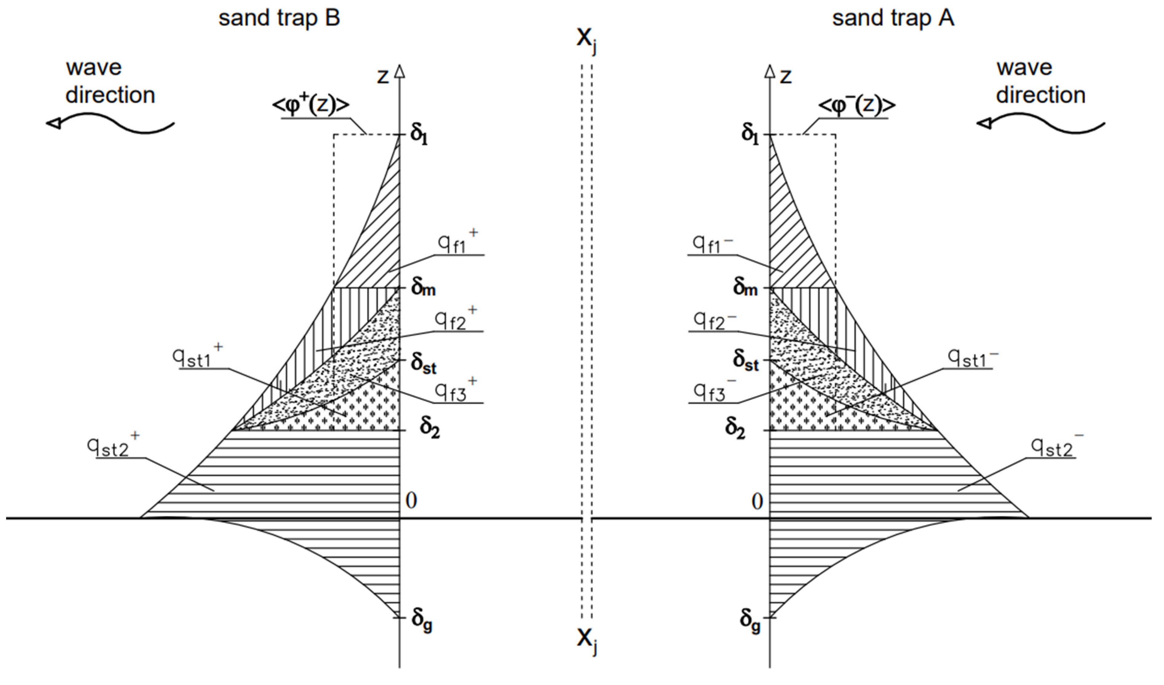
2.1. Sediment Transport during the Wave Crest and Trough

The present study assumed that as a result of tangential shear stresses acting on the bottom varying during the wave period, the sediment is immediately lifted off the bottom and set in motion. Thus, there is an immediate “response” of the bottom to the hydrodynamic conditions varying during the wave period. As a result of this response—under conditions of hydrodynamic equilibrium [37]—the flux of sediment lifted from the bottom at each time instant is equal to the flux of sediment falling to the bottom, and all sediment in motion in the suspended and bedload regime comes exclusively from the bottom of the considered area.

It was postulated that due to the different nature of physical processes occurring at different distances from the bottom, it is necessary to use different assumptions and equations to describe the vertical structure of sediment transport. The basic multilayer model [36,38] presents three main layers with separated sublayers.

The first layer of the model is characterized by a very high concentration of sediment in the immediate vicinity; i.e., directly above and below the conventional bottom line, where transport motion dominates. The second layer, the contact layer, is also characterized by a high concentration, but lower enough that vertical grain sorting is possible. The third layer is an area of well-sorted sediments in suspension, where a very low concentration is found.

It was assumed [36,38] that in a motional layer of densely compacted sediment, all sediment fractions, at each level from the bottom, move at a velocity equal to the velocity of the mixture at that level. Therefore, it was assumed that the interactions between sediment fractions are strong enough that the finer fractions are slowed down by the coarser fractions. The model also accounts for the fact that the most intense vertical sorting of sediment occurs in the contact layer. Turbulent water pulsations and chaotic grain collisions cause the magnitudes of instantaneous velocity u (z,t) and concentration c (z,t) to vary for different fractions in the contact layer.

The model’s assumption of an instantaneous bottom response to bottom friction varying over the wave period makes it difficult to account for the effects of phase lags on sediment transport. In addition, the model does not describe the additional effects of vertical sorting of very fine fractions, which results in these fractions being lifted high above the bottom and simultaneous bottom loss.

When analyzing the situation in which we considered the components of sediment transport involving fine and very fine fractions, due to the different nature of physical processes occurring at different distances from the bottom, several layers could be distinguished to facilitate the description of the vertical structure of the wave induced sediment fluxes flowing out of the control area. Figure 1 presents a schematic of the vertical structure of sediment fluxes in wave motion over a flat bottom, divided into the crest and trough phases. The positive direction of sediment transport is described according to the wave direction (Figure 1). The instantaneous intensity during the wave period of sediment transport in the calculation profile x_j of the control area, during the wave crest and trough, respectively, can be described by the equation:

$$q^{+/-}(t)={{\displaystyle \int }}_{{\delta }_g}^0{\phi }^{+/-}(z,t)dz+{{\displaystyle \int }}_0^{\delta }{\phi }^{+/-}(z,t)dz,$$

(1)

where φ^+/−(z,t) is the elementary instantaneous flux during the wave crest and trough, respectively, described as:

$${\phi }^{+/-}(z,t)=u^{+/-}(z,t) c^{+/-}(z,t),$$

(2)

where u^+/−(z,t) and c^+/−(z,t) are the instantaneous velocity and sediment concentration during the wave crest and trough, respectively.

It was postulated that the total integrated flux with the transport intensity $q^{+/-}$ of sediment is composed of the following components, which are the sum over depth and over time of the crest and trough elemental fluxes:

• Integrated fluxes outgoing from the control area with the intensity of $q_{st}^{+/-}$ transporting sediment grains to adjacent control areas, in both directions. It is the part of integrated total flux with the intensity of $q^{+/-}$, which in the experiment described in this paper was retained in the traps on both sides of the control area. It was postulated [37] that the movement of a packet of grains z_k in sediment fluxes $q_{st}^{+/-}$ follows horizontal projection trajectories of different but equally likely (with probability p = 1/K) lengths Δx_k, where:

$$q_{st}^{+/-}={{\displaystyle \sum }}_{k=1}^K\frac{{( q_{st}^{+/-})}_k}{K}=(1-n_p)\frac{\Delta x_k^{+/-}}{\Delta t}(z_k),$$

(3)

where ∆t is the duration of $q_{st}^{+/-}$ and n_p is the porosity of the sediment (Figure 2);

• Integrated fluxes returning to the control area with the intensity of $q_{f3}^{+/-}$ transporting suspended sediment within the boundary layer of δ_m thickness, defined according to the multilayer model [36,38]. These fluxes are the result of phase lags between water and sediment. These effects cause grains outgoing from the control area in the crest and trough phases to return and be retained in the control area by fluxes outgoing from the trough and crest phases;

• Integrated return fluxes $q_{f1}^{+/-}$ and $q_{f2}^{+/-}$ of sediments suspended high above the bottom and also above the boundary layer ($q_{f1}^{+/-}$). Fluxes $q_{f1}^{+/-}$ and $q_{f2}^{+/-}$ result from the suspension of a large number of very fine sediment grain fractions above the bed, as a consequence of vertical sorting of the granulometrically heterogeneous sediment.

It is worth noting that the return fluxes of suspended sediment $q_{f1}^{+/-}$,$q_{f2}^{+/-}$ and $q_{f3}^{+/-}$(Figure 1) mix with each other and form a depth-averaged flux in the return phase:

$$\langle {\phi }^{+/-}(z)\rangle =\frac{q_{f1}^{+/-}+q_{f2}^{+/-}+q_{f3}^{+/-}}{({\delta }_1-{\delta }_2)}.$$

(4)

Moreover, it is worth noting that an increase in the number of very fine fractions of grains suspended high above the bottom means a loss of these fractions in the bottom, and thus an increase in the bottom roughness and resistance of grain movement. The coarser the grains remain at the bottom, the wider the friction zone of grains becomes. However, as the number of very fine fractions above the bottom increases, their average concentration over depth increases, and as a result, these fractions may form a ring around coarser grains at the bottom, thus facilitating their slip during shearing. On the other hand, in the case of a bottom composed of homogeneous sediments, the lack of vertical sorting of very fine grains high above the bed causes the return flows to reduce only to the flux $q_{f3}^{+/-}.$ Only the presence of bottom forms means a further increase in total return flux at the expense of a radically reduced flux $q_{st}^{+/-}$, as evidenced by experimental data [27]. At this point, it is also worth emphasizing that the increased content of fine fractions in the bottom means an increase in the flux $q_{f3}^{+/-}$ at the expense of the flux $q_{st1}^{+/-}$ (Figure 2). In turn, an increase in hydrodynamic interactions on the bottom results in an increase in fluxes $q_{f1}^{+/-}$,$q_{f2}^{+/-}$, and $q_{f3}^{+/-}$, as well as $q_{st}^{+/-}$.

It was postulated that the total transport ${(q^{+/-})}_j$ in the profile $x_j$ (Figure 1) in the crest and trough, respectively, is the sum of outgoing fluxes $(q_{st}^{+/-}){ }_j={(q_{st1}^{+/-})}_j+{(q_{st2}^{+/-})}_j$ from the computational area and returning ${(q_f^{+/-})}_j$ to this area, whereby ${(q_f^{+/-})}_j={(q_{f1}^{+/-})}_j+{(q_{f2}^{+/-})}_j+{(q_{f3}^{+/-})}_j$. The total bottom erosion z in the computational area is the result of the sum of outgoing ${(q_{st}^{+/-})}_j$, return ${(q_f^{+/-})}_j$, and incoming fluxes from adjacent computational areas ${(q_{st}^{+})}_{j-1}$ and ${(q_{st}^{-})}_{j+1}$. Bottom erosion caused by only outgoing fluxes ${(q_{st}^{+})}_j$ and ${(q_{st}^{-})}_j$ is equal to the sum of the absolute values of these fluxes [8,36]. Such a situation is observed when the bottom is composed only of sediments with i-th fractions with diameter d_i > 0.20 mm. Then, the following relation applies: ${(q_{st}^{+/-})}_j={(q^{+/-})}_j$. When the bottom is composed of sediments with a content of fine fractions (but without very fine fractions), phase lags cause that the flux-induced erosion of the bottom ${(q_{st}^{+/-})}_j$ can be described (following [36]) by a flux $2\left|q^{-}\right|+{(q_{net})}_{meas.}$, where the magnitude $\left|q^{-}\right|$ is proposed to be described by the Kaczmarek et al. 2022 model, while ${(q_{net})}_{meas.}$ is the magnitude determined from measurements.

2.2. Aim and Scope of the Study

The primary aim of the measurements was to collect experimental data documenting the vertical structure of the total sediment fluxes with the rate $q^{+/-}$ in the crest and trough phases, respectively, as well as the magnitudes of both the flux rate $q_{st}^{+/-}$ of sediment flow in both directions from the computational area to the adjacent control areas (and retained in the traps) and the granulometric composition of these sediments on both sides of the initial area. Knowledge of these magnitudes was essential for proper assessment of bathymetry changes in the computational area.

Achievement of the objective was carried out experimentally in two stages. The first involved the experimental identification using the particle image velocimetry (PIV) method of return fluxes $q_{f1}^{+/-}, q_{f2}^{+/-}$, and $q_{f3}^{+/-}.$ The second stage of experimental work included measurements of fluxes $q_{st}^{+}$ and $q_{st}^{-}$, along with a determination of the granulometric composition of transported sediments. The experimental results were then compared with the results of a theoretical analysis based on a three-layer model of heterogeneous sediment transport [36]. Due to the fact that this model did not take into account the effects of vertical sorting of sediments containing the i-th of very fine fractions in the diameter range d_i < 0.20 mm, it neglected the effects of phase lags of fine fractions in this range, and did not describe the influence of these fractions on the transport volume $q_{st}^{+/-}$, so a modification of this model including the aforementioned effects was proposed.

2.3. Experimental Investigation

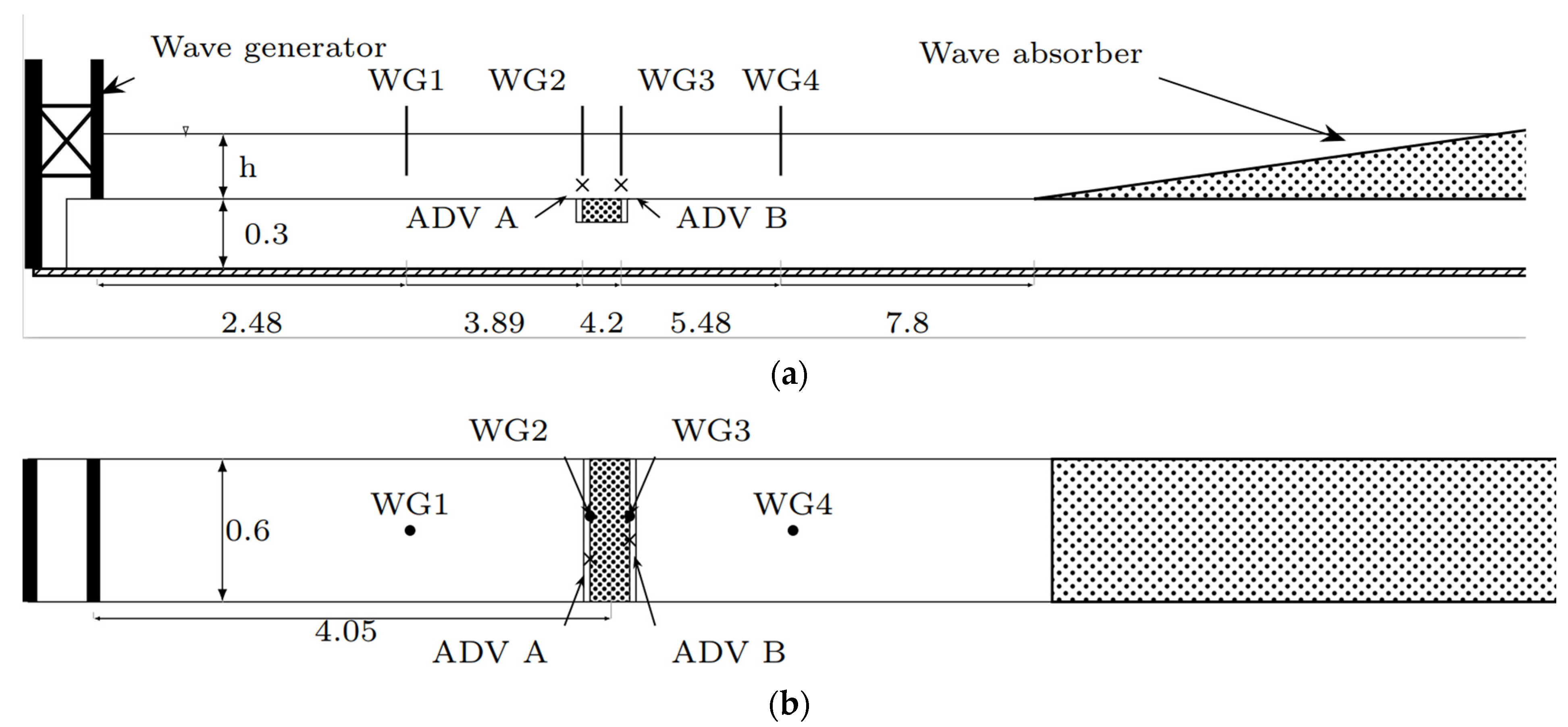
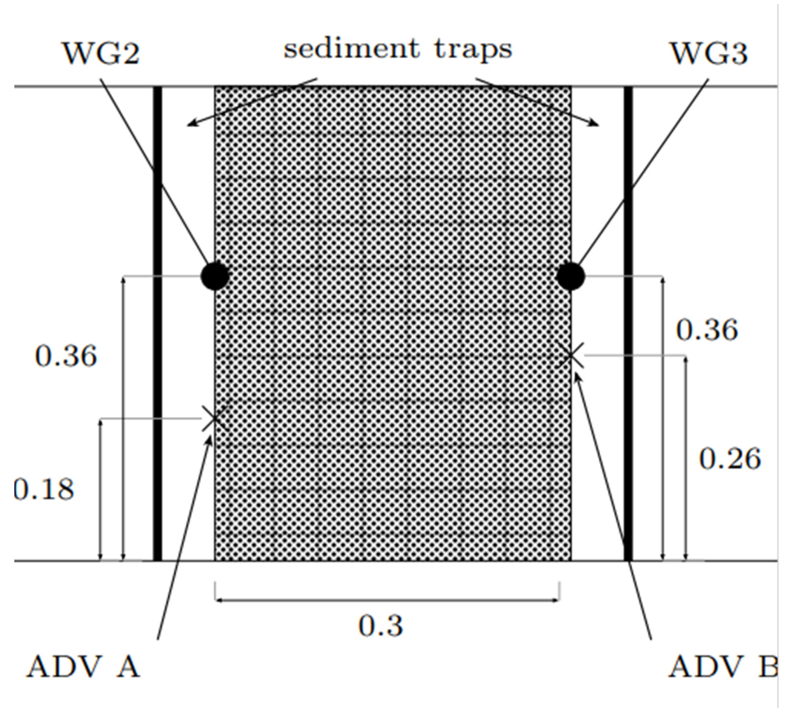
2.3.1. Experimental Setup

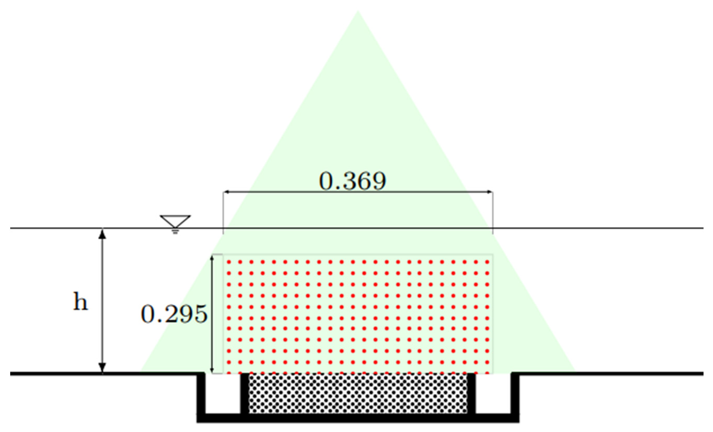
The experimental objectives were achieved in the wave-current flume in the hydraulic laboratory of the Institute of Hydro-Engineering at the Polish Academy of Sciences in Gdańsk in 2020. The channel was equipped with measuring and supporting devices necessary to conduct the research. The wave tank with glass walls was 64 m long and 0.6 m wide. Operational water depths typically ranged from 0.2 m to 0.8 m. The channel was equipped with vertical glass walls parallel to each other that transmitted light, allowing unobstructed observation of ongoing studies and the use of particle image velocimetry (PIV) imaging anemometry techniques [2 MP]. Waves were generated by a piston-type generator installed at the upper end of the trough. The described sand bed experiments were conducted in a dedicated section of the flume, as shown in Figure 3. The section was bounded by a wavemaker paddle and wave absorber to eliminate the wave reflection effect. Installation of the trap structure in the sandy bottom required some modifications to be made to the original geometry of the wave flume. The original bottom was raised by 0.3 m, and then the traps were inserted between the new bottom structure. Tests were conducted for two water levels corresponding to the depths h = 0.28 m and h = 0.36 m in order to optimize the research by presenting weaker (0.36 m) and stronger (0.28 m) hydrodynamic conditions.

Twenty-four measurement tests (twelve each for two water depths) were conducted to measure the magnitude of sediment transport over a flat bottom. All experiments involved simultaneous sampling of surface sediments trapped in traps on either side of a control area filled with sandy sediment with very fine fractions. A set of resistance probes that recorded data at a sampling rate of 100 Hz was used to measure changes in water surface elevation. Measurements of water particle flow velocity were conducted using acoustic doppler velocimeter (ADV) ultrasonic velocimeters recording at 25 Hz [1 MP].

In order to measure the transport of noncohesive and granulometrically nonhomogeneous sediment of any given granulometric distribution, the authors’ constructions of a sand trap were used. The construction consisted of a main “tube” (sand section) and “traps” (sediment traps) composed of waterproof plywood and plastic boards that were painted black and installed in front of and behind the sand section. The model consisted of two traps (A and B) with dimensions of 100 × 560 × 100 mm and a box/tube located between the traps with dimensions of 300 × 560 × 100 mm.

Measurement tests were conducted for four sediments, each for two water depths (0.28 m and 0.36 m), without changing the wave conditions (the wave height, wave period, and experiment duration remained constant).

The wavemaker generated trains of regular waves with predefined characteristics; i.e., wave period T and wave height H. Waves were recorded using two wave probes placed along the length of the channel, upstream and downstream of the sand sections.

Table 1. Basic data of the flat bottom experiment—IBW PAN 2020.

Parameter	Symbol	Value	Unit
Water depth	h0	0.28/0.36	m
Wave height	Hw	0.12	m
Test duration	Tw	10	min
Wave peak period	Tp	3.0	s
Representative diameter of bottom-building sediment grains	d50	A: 0.38 B: 0.32 C: 0.25 D: 0.14	mm
Sediment density	ρs	2.62	g/cm3
Liquid density	ρw	1.00	g/cm3
Sediment porosity	np	0.4	–

shows the basic parameters of the experiment, in which, among others, the time-averaged (from the two wave probes) wave height in each test was denoted according to the H_w wave height.

2.3.2. PIV System

In the first stage of the experiments, particle image velocimetry (PID) measurements of sand kinematics were conducted. The wave tests covered hydrodynamic and sediment conditions from the previous stage with changes introduced to the number and duration of tests, which was set to 5 min. Experimentally investigated wave-sediment scenarios are characterized in

Table 2. Summary of PIV wave test cases.

Test No.	Sand	h	T	H
T0134	A	0.28	3.0	0.12
T0135	B	0.28	3.0	0.12
T0136	C	0.28	3.0	0.12
T0137	D	0.28	3.0	0.12
T0128	A	0.36	3.0	0.12
T0129	B	0.36	3.0	0.12
T0130	C	0.36	3.0	0.12
T0131	D	0.36	3.0	0.12

.

In this stage, the 2D Flowmaster PIV system comprising a high-speed 1 MP camera and a high-power dual laser operating at a maximum repetition rate of 50 Hz was used. The layout of the PIV apparatus and its location in the flume is presented in Figure 4 and Figure 5. Usually, the PIV system is applied to retrieve the wave field in terms of water velocities from the images of illuminated seeding (e.g., hollow glass spheres) suspended in water. However, in the present laboratory setup, sand particles took the role of seeding, and the system was able to estimate sand velocities under the given hydrodynamic excitation. For the principle of PIV measurements, the reader is referred to papers on the use of PIV techniques in experimental fluid mechanics [39,40] or previous PIV applications to various problems of wave hydrodynamics performed in the IHE flume [41,42,43]. Nonetheless, a short description of applied methods is provided below.

Sand particle velocity measurements were performed in a plane parallel to the direction of waves and flume walls. The PIV camera traced sand particle displacements by recording images in a 0.397 m × 0.317 m field of view with a fixed sampling frequency of 50 Hz. In the present study, the multipass method with a decreasing size of interrogation windows was used in order to increase the accuracy of the velocity calculation in smaller subareas of interest by reducing the error of measurements to approximately 0.1% of the mean registered velocity [44]. Based on the displacement in interrogation windows and a given time increment (1/50 s), two vector components were calculated. A summary of technical parameters and processing methods used in the present PIV setup is provided in

Table 3. PIV system description in terms of technical components and processing methods.

System Item/Method	Description/Parameters
Data Acquisition:
Light source	Dual-head Nd-YAG 532-nm laser, 2 × 50 mJ @ 50 Hz
Camera	Imager Pro HS 500 double-frame CCD, 1280 × 1024 @ 520 fps
Data Processing:
Vector calculation	Time series of single frames: cross-correlation; multipass with decreasing window size; iterations: - Initial step: 128 × 128 pixel window, single pass,    50% overlap - Final steps: 64 × 64 pixel window, two passes,    75% overlap
	Options: - Image correction; - High-accuracy mode for final passes;
Masking functions	Geometric mask

.

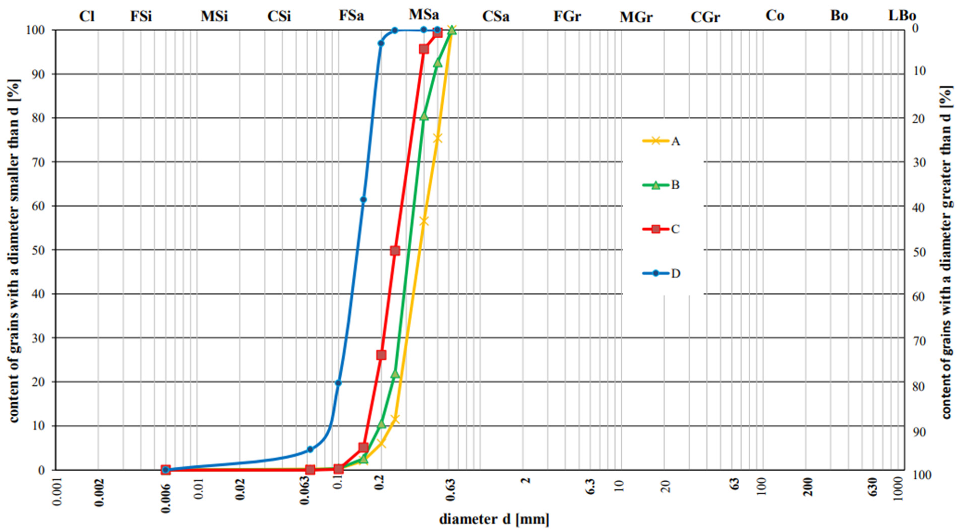
2.3.3. Sediment Transport and Grain Distribution Measurements

Four types of quartz sands with the granulometric characteristics summarized in

Table 4. Granulometric characteristics of the studied sands.

Type of Sand	d90/d50/d10
A. Coarse quartz sand	0.58/0.38/0.24
B. Medium quartz sand	0.48/0.32/0.20
C. Fine quartz sand	0.38/0.25/0.16
D. Very fine quartz sand	0.19/0.14/0.08

were selected for the experiments.

Sands were subjected to granulometric analysis. For this purpose, a MikroLAB sieve shaker (model: LPzE-2e) was used. Measurements were made using the “dry” method for all collected sediment samples. Before the tests, samples were collected from a container filled with the sediment prepared for testing, while after each test, a sample was taken from traps A and B. Samples collected from traps were dried at 100 °C for 24 h before granulometric analysis. The results were essentially identical for all measurements taken. The cumulative grain size curves of the four sediments are shown in Figure 6.

As can be seen in the grain size curves prepared, the sands analyzed could be divided into two types:

• Sandy with a very high proportion of fine fractions (d₅₀ < 0.20 mm; sand D: grain content d_i < 0.20 mm = 97%);
• Sandy with low content of fine fractions (d₅₀ ≥ 0.20 mm; grain content d_i < 0.20 mm: sand A = 6%, B = 10.5%, C = 26%).

Each measurement test was performed according to the following procedure. Waves with preset characteristics were generated for 10 min (Table 1). After the wave projection was completed, measurements of bottom bathymetry in the central part of control area and sand mass in both sediment traps were made. A total of 24 measurement series were conducted covering four sand types and two water depths with three repetitions of each case.

Bathymetric measurements were conducted using a bar with rods with flat weights attached to their end.

During the crest, sediment was carried into trap B, and during the trough, into trap A. At the end of each wave projection, in order to determine the volume of accumulated sediment in traps, the sediment had to be transported out of the channel. For this purpose, the syphoning method was used. Using silicon tubing, the water–sediment mixture was pumped out of the extreme boxes into two separate boxes. The samples were then transferred to flasks, which were filled with water to a known volume. The flasks with sediment and water were weighed, and the volume of sediment extracted from each of the traps was determined.

3. Results and Discussion

3.1. Theoretical Investigations

3.1.1. Sediment Transport during the Wave Crest and Trough Phase

In the theoretical analysis, it was assumed that the return fluxes $q_{f1}^{+/-}$ and $q_{f2}^{+/-}$ resulted from the suspension of a large number of very fine fractions in the range d_i < 0.20 mm high above the bottom, as a result of vertical sorting of granulometrically heterogeneous sediment. Furthermore, it was assumed that the return flow $q_{f3}^{+/-}$ resulted from phase lags between water and fine fractions in the range of d_i < 0.20 mm. A theoretical analysis should be based on a three-layer heterogeneous sediment model [36]. However, this model does not take into account the effects of additional vertical sorting of very fine sediment fractions and neglects the effects of phase lags of fine fractions. Therefore, a modification of this model based on experimental results was proposed.

It was proposed to describe theoretical fluxes ${(q_{st}^{+/-})}_{calc.}$ (calculated using the Kaczmarek et al. 2022 model) as a sum of fluxes of fine and very fine fractions ${(q_f^{+/-})}_{calc.}$ with a diameter of d_i < 0.20 mm and coarse fractions ${(q_c^{+/-})}_{calc.}$ with diameter of d_i ≥ 0.20 mm, as follows:

$${(q_{st}^{+/-})}_{calc.}={(q_f^{+/-})}_{calc.}+{(q_c^{+/-})}_{calc.},$$

(5)

where:

$${(q_f^{+/-})}_{calc.}={{\displaystyle \sum }}_{i=1}^{N_f}{n}_{fi}{(q_{fi}^{+/-})}_{calc.},$$

(6)

$${(q_c^{+/-})}_{calc.}={{\displaystyle \sum }}_{i=N_f}^N{n}_{ci}{(q_{ci}^{+/-})}_{calc.},$$

(7)

where:

$n_{fi}$—proportion of the i-th fine and very fine fraction (d_i < 0.2 mm) in the input mixture;

$n_{ci}$—proportion of the i-th coarse fraction (d_i ≥ 0.2 mm) in the input mixture;

${(q_{fi}^{+/-})}_{calc.}$—transport rate of the i-th fine and very fine fraction (d_i < 0.2 mm), calculated using the Kaczmarek et al. 2022 model;

${(q_{ci}^{+/-})}_{calc.}$—transport rate of the i-th coarse fraction (d_i ≥ 0.2 mm), calculated using the Kaczmarek et al. 2022 model;

i = N_f—fraction with a diameter of d_i = 0.2 mm.

Modification of the flux calculation results (5) was proposed based on the correction factors ${\beta }_1^{+/-}$ and ${\beta }_2^{+/-}$ determined from flux measurements ${(q_{st}^{+/-})}_{meas.}$ as follows:

$$q_{st}^{+}={\beta }_1^{+}{(q_f^{+})}_{calc.}+{\beta }_2^{+}{(q_c^{+})}_{calc.},$$

(8)

$$q_{st}^{-}={(q_f^{-})}_{calc.}+{(q_c^{-})}_{calc.}+{\beta }_1^{-}{(q_f^{+})}_{calc.}+{\beta }_2^{-}{(q_c^{+})}_{calc.},$$

(9)

postulating the equality of fluxes $q_{st}^{+/-}$=${(q_{st}^{+/-})}_{meas.}$, where:

$${(q_{st}^{+/-})}_{meas.}={\displaystyle \sum }_{i=1}^{N_f}{(n_{fi}^{+/-})}_{meas.}{(q_{st}^{+/-})}_{meas.}+{\displaystyle \sum }_{i=N_f}^N{(n_{ci}^{+/-})}_{meas.}{(q_{st}^{+/-})}_{meas.}.$$

(10)

where:

$n_{fi}^{+/-}$—proportion of the i-th fine and very fine fraction (d_i < 0.2 mm) in the mixture collected from the trap;

$n_{ci}^{+/-}$—the proportion of the i-th coarse fraction (d_i ≥ 0.2 mm) in the mixture collected from the trap.

The values of correction factors can be found using relations (8), (9), and (10) as follows:

$${\beta }_1^{+}=\frac{{(q_{st}^{+})}_{meas.}{{\displaystyle \sum }}_{i=1}^{N_f}{(n_{fi}^{+})}_{meas.}}{{{\displaystyle \sum }}_{i=1}^{N_f}{n}_{fi}{(q_{fi}^{+})}_{calc.}},$$

(11)

$${\beta }_2^{+}=\frac{{(q_{st}^{+})}_{meas.}{{\displaystyle \sum }}_{i=N_f}^N{(n_{ci}^{+})}_{meas.}}{{{\displaystyle \sum }}_{i=N_f}^N{n}_{ci}{(q_{ci}^{+})}_{calc.}},$$

(12)

$${\beta }_1^{-}=\frac{{(q_{st}^{-})}_{meas.}{{\displaystyle \sum }}_{i=1}^{N_f}{(n_{fi}^{-})}_{meas.}-{{\displaystyle \sum }}_{i=1}^{N_f}{n}_{fi}{(q_{fi}^{-})}_{calc.}}{{{\displaystyle \sum }}_{i=1}^{N_f}{n}_{fi}{(q_{fi}^{+})}_{calc.}},$$

(13)

$${\beta }_2^{-}=\frac{{(q_{st}^{-})}_{meas.}{{\displaystyle \sum }}_{i=N_f}^N{(n_{ci}^{-})}_{meas.}-{{\displaystyle \sum }}_{i=N_f}^N{n}_{ci}{(q_{ci}^{-})}_{calc.}}{{{\displaystyle \sum }}_{i=N_f}^N{n}_{ci}{(q_{ci}^{+})}_{calc.}},$$

(14)

3.1.2. Grain Size Distributions of Transported Sediments

Apart from the changes occurring in the magnitudes of transported sediment with the proportion of fine and very fine fractions in the crest and trough phases, there also are obvious changes in the granulometric composition of the transported grain magnitude. The proportion of fine and coarse fractions transported during the wave crest; i.e., measured in the trap, can obviously be described by the sum of the i-th fractions while distinguishing between fine fractions (d_i < 0.2 mm) and coarse fractions (d_i ≥ 0.2 mm):

$${(n_f^{+/-})}_{meas.}={\displaystyle \sum }_{i=1}^{N_f}{(n_{fi}^{+/-})}_{meas.},$$

(15)

$${(n_c^{+/-})}_{meas.}={\displaystyle \sum }_{i=N_f}^N{(n_{ci}^{+/-})}_{meas.}.$$

(16)

The proportion of fine and very fine ${(n_f^{+/-})}_{calc.}$ and coarse ${(n_c^{+/-})}_{calc.}$ fractions in the trap, as calculated using the model of Kaczmarek et al. 2022, can be described as follows:

$${(n_f^{+/-})}_{calc.}=\frac{{{\displaystyle \sum }}_{i=1}^{N_f}{n}_{fi}{(q_{fi}^{+/-})}_{calc.}}{{{\displaystyle \sum }}_{i=1}^{N_f}{n}_{fi}{(q_{fi}^{+/-})}_{calc.}+{{\displaystyle \sum }}_{i=N_f}^N{n}_{ci}{(q_{ci}^{+/-})}_{calc.}},$$

(17)

$${(n_c^{+/-})}_{calc.}=\frac{{{\displaystyle \sum }}_{i=N_f}^N{n}_{ci}{(q_{ci}^{+/-})}_{calc.}}{{{\displaystyle \sum }}_{i=1}^{N_f}{n}_{fi}{(q_{fi}^{+/-})}_{calc.}+{{\displaystyle \sum }}_{i=N_f}^N{n}_{ci}{(q_{ci}^{+/-})}_{calc.}}.$$

(18)

To calculate the proportion of fine and very fine (d_i < 0.2 mm) and coarse (d_i < 0.2 mm) fractions for any given granulometric distribution of noncohesive sediments with the proportion of very fine and fine fractions, it is suggested to use the correction factors described by relations (11), (12), (13), and (14). Then the proportion of fine and very fine fractions ${(n_f^{+})}_{st}$ and coarse fractions ${(n_c^{+})}_{st}$ caught in the trap in the crest phase can be calculated as the transport ratio of fine/coarse fractions to the total transport in the crest phase, according to the following equations:

$${(n_f^{+})}_{st}=\frac{{\beta }_1^{+}{{\displaystyle \sum }}_{i=1}^{N_f}{n}_{fi}{(q_{fi}^{+})}_{calc.}}{{{\displaystyle \sum }}_{i=1}^{N_f}{n}_{fi}{(q_{fi}^{+})}_{calc.}+{{\displaystyle \sum }}_{i=N_f}^N{n}_{ci}{(q_{ci}^{+})}_{calc.}},$$

(19)

$${(n_c^{+})}_{st}=\frac{{\beta }_2^{+}{{\displaystyle \sum }}_{i=N_f}^N{n}_{ci}{(q_{ci}^{+})}_{calc.}}{{{\displaystyle \sum }}_{i=1}^{N_f}{n}_{fi}{(q_{fi}^{+})}_{calc.}+{{\displaystyle \sum }}_{i=N_f}^N{n}_{ci}{(q_{ci}^{+})}_{calc.}}.$$

(20)

In the trough phase, the magnitude ${(n_f^{-})}_{st}$ and ${(n_c^{-})}_{st}$ can be described as follows:

$${(n_f^{-})}_{st}=\frac{{{\displaystyle \sum }}_{i=1}^{N_f}{n}_{fi}{(q_{fi}^{-})}_{calc.}+{\beta }_1^{-}{{\displaystyle \sum }}_{i=1}^{N_f}{n}_{fi}{(q_{fi}^{+})}_{calc.}}{{{\displaystyle \sum }}_{i=1}^{N_f}{n}_{fi}{(q_{fi}^{-})}_{calc.}+{{\displaystyle \sum }}_{i=N_f}^N{n}_{ci}{(q_{ci}^{-})}_{calc.}+{\beta }_1^{-}{{\displaystyle \sum }}_{i=1}^{N_f}{n}_{fi}{(q_{fi}^{+})}_{calc.}+{\beta }_2^{-}{{\displaystyle \sum }}_{i=N_f}^N{n}_{ci}{(q_{ci}^{+})}_{calc.}},$$

(21)

$${(n_c^{-})}_{st}=\frac{{{\displaystyle \sum }}_{i=N_f}^N{n}_{ci}{(q_{ci}^{-})}_{calc.}+{\beta }_2^{-}{{\displaystyle \sum }}_{i=N_f}^N{n}_{ci}{(q_{ci}^{+})}_{calc.}}{{{\displaystyle \sum }}_{i=1}^{N_f}{n}_{fi}{(q_{fi}^{-})}_{calc.}+{{\displaystyle \sum }}_{i=N_f}^N{n}_{ci}{(q_{ci}^{-})}_{calc.}+{\beta }_1^{-}{{\displaystyle \sum }}_{i=1}^{N_f}{n}_{fi}{(q_{fi}^{+})}_{calc.}+{\beta }_2^{-}{{\displaystyle \sum }}_{i=N_f}^N{n}_{ci}{(q_{ci}^{+})}_{calc.}}.$$

(22)

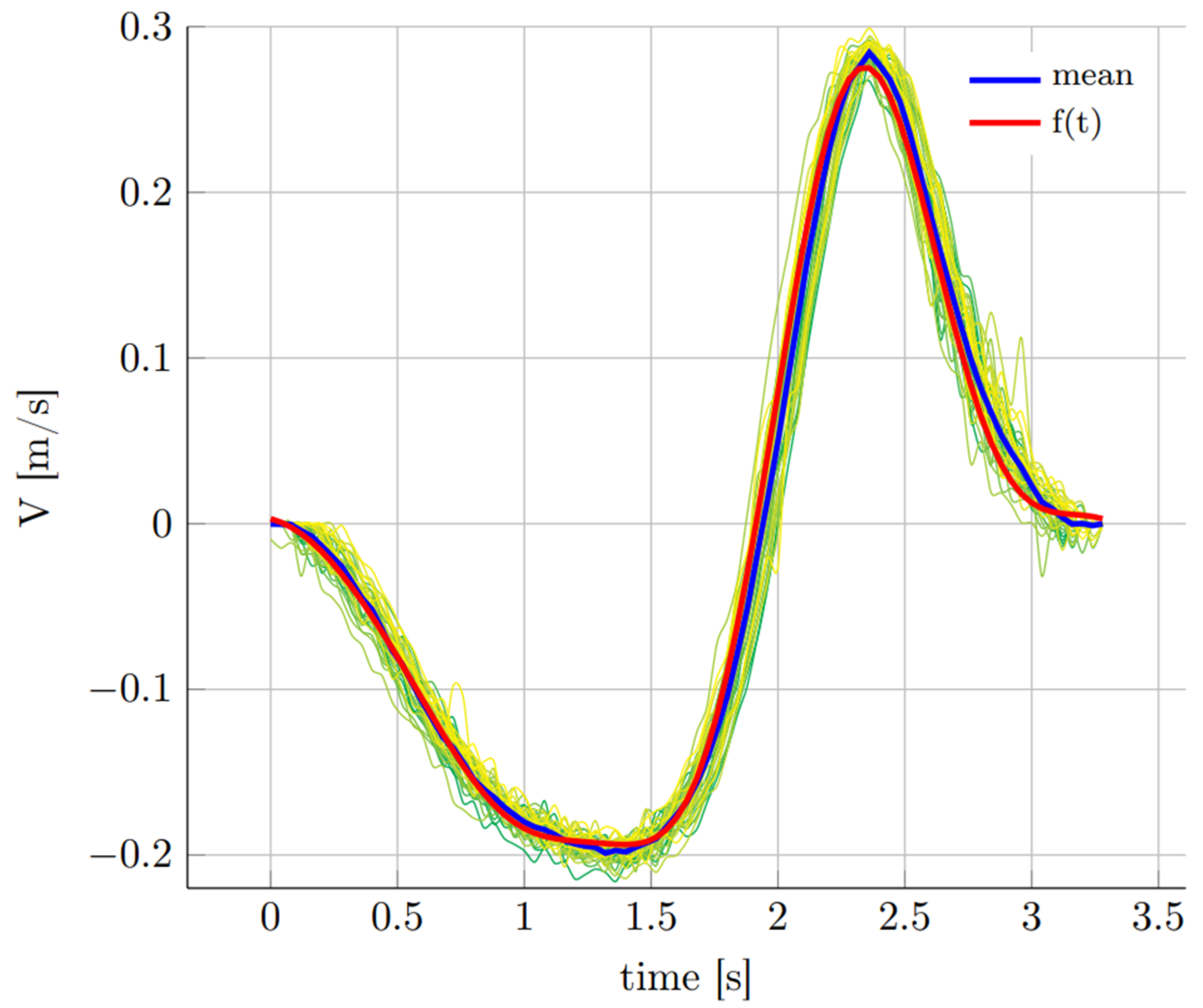
3.2. Free Stream Velocity Measurements

The free stream velocities are defined as the surface-wave-induced orbital velocity at the edge of the wave boundary layer [45]. The velocities were estimated based on ADV records. These measurements were performed at a distance of 6 cm above the sand box edges. The exact localization of upstream (ADV A) and downstream (ADV B) probes is presented at Figure 4. To estimate the characteristic period of the along-flume (the X) component of particle velocity, it was divided according to the series of records covering one wave period.

The characteristic period of the along-flume particle velocity component was determined by extracting the velocities covering one wave period from the ADV record. The gathered series of velocities were used to estimate the characteristic distribution of velocities during one wave period by taking the mean value at a particular time. The corresponding curve, which is denoted by the blue line in Figure 7, was decomposed into a Fourier series. The estimated Fourier coefficients were used to reproduce the mean velocity with n = 4 harmonics according to Equation (23):

$$\mathrm{f}(\mathrm{t})=0.5{\mathrm{a}}_0+{{\displaystyle \sum }}_{\mathrm{i}=1}^{\mathrm{i}=\mathrm{n}}({\mathrm{a}}_{\mathrm{n}}\cos (\mathrm{n}2\mathsf{\pi }\mathrm{t})+{\mathrm{b}}_{\mathrm{n}}\sin (\mathrm{n}2\mathsf{\pi }\mathrm{t})).$$

(23)

The resulting curve f(t) is denoted by the red line in Figure 7. Moreover, the procedure provided an analytical solution that was used as an input for the numerical model. The Fourier series coefficients are summarized in

Table 5. Summary of Fourier series coefficients used as inputs to the numerical model.

Test No.	0.5*a0	a1	b1	a2	b2	a3	b3	a4	b4	ADV
T = 3 H = 0.12 H = 0.28	−0.0182	0.0259	−0.1934	−0.0414	0.0616	−0.0338	0.0137	−0.0011	−0.0097	A
	−0.0198	0.0509	−0.1758	−0.0641	0.0550	0.0342	0.0293	0.0017	−0.0110	B
T = 3 H = 0.12 H = 0.36	−0.0219	0.0148	−0.1876	−0.0249	0.1035	0.0591	−0.0387	−0.0305	−0.0105	A
	−0.0241	−0.0174	−0.1824	0.0257	0.0858	0.0292	−0.0602	−0.0332	0.0098	B

.

The characteristic record of horizontal velocity was obviously generated by the nonlinear wave. The asymmetry of crest to trough of these waves generated a higher horizontal velocity under the crest than under the trough, which led to the near-bed horizontal velocity skewness. This can be clearly seen in Figure 7, especially for negative velocities recorded under the passing wave trough. This affected the mechanism of sediment movement near the sea bottom [46].

3.3. PIV Measurements

The analysis of the PIV results allowed instantaneous sand velocities to be calculated for a selected time frame. The respective horizontal and vertical component sand velocities u and w were resolved for the entire area of interest. The horizontal velocity u was then used to determine the instantaneous sediment fluxes in a layer adjacent to the bottom as:

$$q_{A/B}=\frac{1}{\delta }{{\displaystyle \int }}_0^{\delta }u(x_{A/B},z,t)dz,$$

(24)

where δ = 0.5 and 2 cm, while x_A = −0.16 m and x_B = 0.16 m. The instantaneous fluxes expressed by (24) were conditionally averaged over one wave period for consecutive waves. This conditional average refers to the negative (opposing the wave) and positive (following the wave) fluxes through the given cross section, which may be expressed as:

$${\widehat{q}}_{A/B}^{+}=\frac{1}{T}{{\displaystyle \int }}_0^T{q}_{A/B}dt, q_{A/B}>0,$$

(25)

$${\widehat{q}}_{A/B}^{-}=\frac{1}{T}{{\displaystyle \int }}_0^T{q}_{A/B}dt, q_{A/B}<0.$$

(26)

Component fluxes were averaged again over a total number of 18 wave periods, and phase-averaged (wave period mean) sediment fluxes in both directions are estimated.

Table 6. PIV estimates of sand fluxes.

δ = 0.5 cm
Case	Trough		Crest
	${\widehat{\mathit{q}}}_{\mathit{A}}$ from Sand Trap	${\widehat{\mathit{q}}}_{\mathit{A}}$ to Sand Trap	${\widehat{\mathit{q}}}_{\mathit{B}}$ to Sand Trap	${\widehat{\mathit{q}}}_{\mathit{B}}$ from Sand Trap
Sand A h = 0.36 m	0.00012 (8.6%)	−0.00020 (4.5%)	0.00009 (6.9%)	−0.00005 (6.3%)
Sand B h = 0.36 m	0.00018 (3.7%)	−0.00025 (5.6%)	0.00009 (8.3%)	−0.00006 (9.6%)
Sand C h = 0.36 m	0.00022 (5.2%)	−0.00025 (3.9%)	0.00007 (13.1%)	−0.00006 (7.1%)
Sand A h = 0.28 m	0.00017 (4.8%)	−0.00028 (6.8%)	0.00014 (11.1%)	−0.00009 (6.8%)
Sand B h = 0.28 m	0.00010 (14.8%)	−0.00022 (8.9%)	0.00008 (21.2%)	−0.00009 (8.7%)
Sand C h = 0.28 m	0.00020 (8.1%)	−0.00026 (5.7%)	0.00006 (16.4%)	−0.00007 (5.3%)
δ = 2.0 cm
Case	Trough		Crest
	${\widehat{q}}_A$  from sand trap	${\widehat{q}}_A$  to sand trap	${\widehat{q}}_B$  to sand trap	${\widehat{q}}_B$  from sand trap
Sand A h = 0.36 m	0.00067 (7.2%)	−0.00061 (7.0%)	0.00016 (9.1%)	−0.00026 (7.3%)
Sand B h = 0.36 m	0.00094 (2.5%)	−0.00091 (8.1%)	0.00020 (10.3%)	−0.00035 (11.2%)
Sand C h = 0.36 m	0.00105 (3.1%)	−0.00091 (5.2%)	0.00021 (15.2%)	−0.00031 (8.5%)
Sand A h = 0.28 m	0.00102 (4.3%)	−0.00117 (7.6%)	0.00042 (17.0%)	−0.00049 (8.6%)
Sand B h = 0.28 m	0.00065 (11.7%)	−0.00072 (10.2%)	0.00024 (24.5%)	−0.00038 (11.4%)
Sand C h = 0.28 m	0.00102 (4.6%)	−0.00112 (7.6%)	0.00016 (12.6%)	−0.00035 (6.4%)

shows the wave-average values of the phase-averaged fluxes ${\widehat{q}}_{A/B}$, which constituted the final result of the present PIV analysis and the experimental basis for validation of the theoretical model. The results in Table 6 are complemented by relative random error estimates in parentheses. In the present analysis, the random error was calculated as the standard deviation of the mean based on transport values for 18 waves.

It should be noted here that in the case of PIV methods, uncertainty of the measurements of sand kinematics is higher when compared with water particle velocity measurements. This results from homogeneity of the seeding in a measurement plane, which is high for water (seeding occupies the entire plane) and low for sand (only wave-induced bursts and clouds of sand near the bottom are captured). Thus, PIV measurements of sand velocity and corresponding mass fluxes could be treated as estimates only in the present analysis. The higher the bottom, the more the error in flux analysis ${\widehat{q}}_{A/B}$ increased, because there, the concentration of sediment c(z) was smaller, and the concentration gradient $\frac{\partial c}{\partial z}$ in the vertical profile increased significantly.

However, the following conclusions can be deduced from the data in Table 6:

1.

As would be expected, the flux ${\widehat{q}}_B$ within the boundary layer (thickness $\delta \approx 0.5 \mathrm{cm}\approx {\delta }_m)$ outgoing from the computational area and directed to the trap (positive values) reached higher values than the absolute values of the flux ${\widehat{q}}_B$ returning to the computational area (Table 6). However, the more very fine fractions in the bottom, the more the outgoing and returning fluxes ${\widehat{q}}_B$ balanced each other. This was understandable, because more very fine fractions in the fluxes $q_{f1}^{+}$, $q_{f2}^{+}$, and $q_{f3}^{+}$ meant a larger (after they were mixed) depth-averaged return flux. As a result, the balancing of the outgoing and returning fluxes ${\widehat{q}}_B$ occurred closer to the bottom, at the boundary of the near-wall layer (Figure 1). As a result, high above the bottom, the returning fluxes ${\widehat{q}}_B$ were larger than those outgoing the control area (Figure 1). This was especially visible in cases of stronger bottom impacts, which was confirmed by observations of ${\widehat{q}}_B$ (Table 6) in the area high above the near-wall layer ($\delta \approx 2.0 \mathrm{cm}$), where the proportion of suspended fine and very fine fractions in this flux was dominant. It is worth noting that the above effect occurred in the crest phase, when it could be expected that the orbital velocities in the returning flux ${\widehat{q}}_B$ were smaller than in the outgoing flux ${\widehat{q}}_B$. In addition, the higher proportion of very fine fractions in the fluxes ${\widehat{q}}_B$ resulting from their elevation above the boundary layer may imply their absence from the bottom, thus causing an increase in the bottom roughness and a decrease in the flux $q_{st}^{+}$ entering the trap;

2.

In the trough phase, the fluxes ${\widehat{q}}_A$ reached absolute values higher than fluxes ${\widehat{q}}_B$ in the crest phase (Table 6). The above observation seemed to be understandable due to the increased presence of very fine fractions in the computational area caused by the returning flux ${\widehat{q}}_B$. However, the increased differences between the absolute values of fluxes ${\widehat{q}}_A$; i.e., those outgoing from the computational area and directed to the trap (negative values) and those returning, clearly indicated a significant contribution $q_{st}^{-}$ in the flux ${\widehat{q}}_A$. This suggested a significant increase in $q_{st}^{-}$ by expanding the flux $q_{st1}^{-}$ at the expense of $q_{f3}^{-}$. On the other hand, the increased amount of very fine fractions in the trough phase implied an increase in the average postdepth concentration of these fractions, and in effect, by forming an envelope around coarse grains, they facilitated their transport. As a result, an increase in the amount of coarse fractions (d_i ≥ 0.20 mm) was to be expected in the flux $q_{st}^{-}$ entering the trap A. The above effects were so strong (Table 5) that even in areas located higher up the bottom ($\delta \approx 2.0 \mathrm{cm}$), but under stronger conditions, the absolute values of the flux ${\widehat{q}}_A ;$ i.e., outgoing from the computational area and directed to the trap, remained larger than the returning flux ${\widehat{q}}_A$, as the latter was formed only by the fluxes $q_{f1}^{-}$ and $q_{f2}^{-}$.

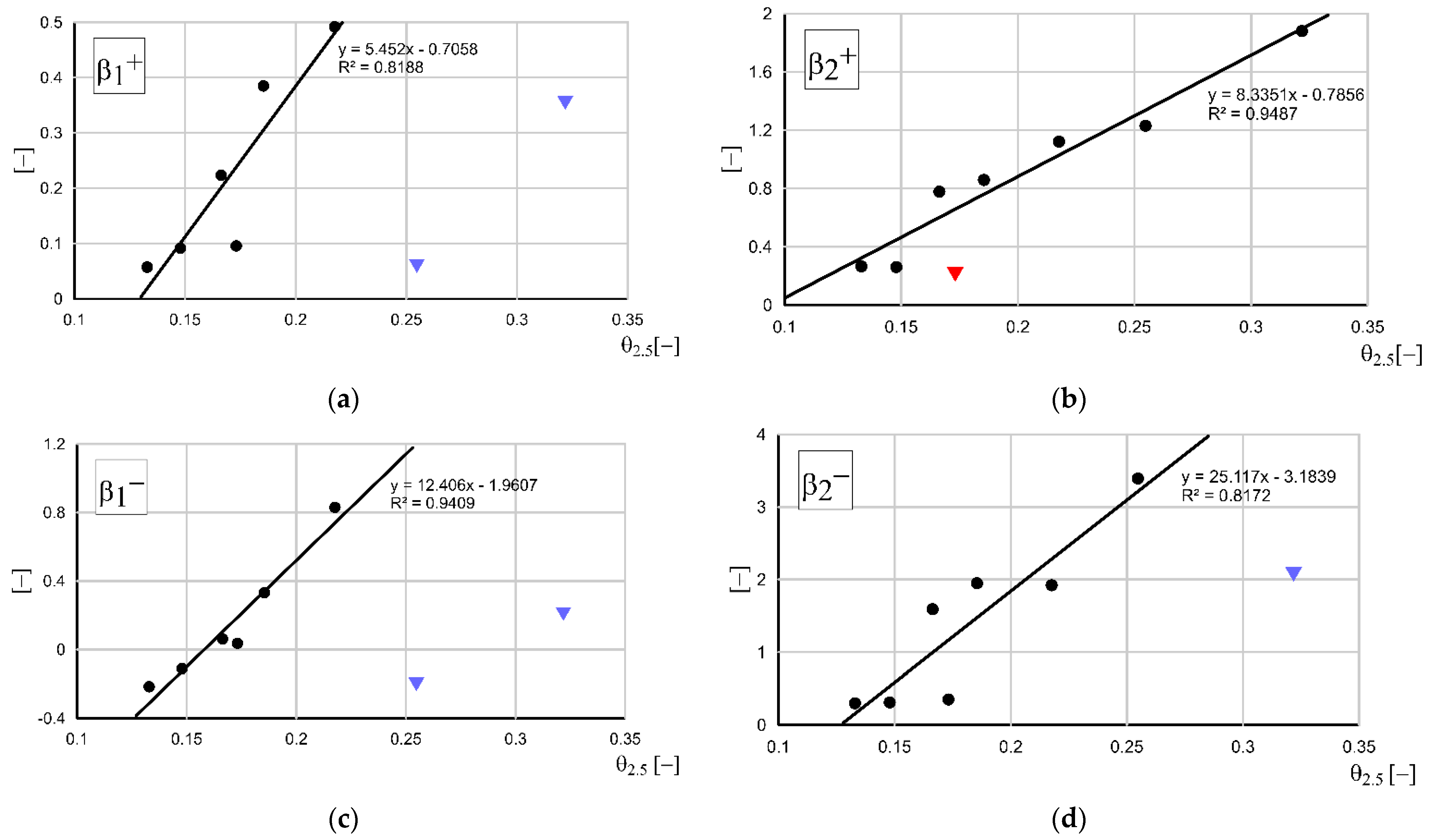
3.4. Correction Factors for Sediment Fluxes

The calculated correction coefficients are shown in Figure 8a–d as a function of Shields’ parameter θ_2.5; i.e., the dimensionless bottom friction calculated using the Kaczmarek et al. 2022 model for the maximum tangential stress during the wave period. The coefficients were calculated using Equations (11) ÷ (14) and then approximated using a correlation curve with a coefficient of determination $R^2\ge 0.80$. In order to obtain such a high value of fit, the few results of the calculated coefficients that deviated significantly from the correlation curve had to be omitted in some cases. The deviations were mainly in the case of sand with a content of very fine grains (type D; d₅₀ = 0.14). In such cases, the arithmetic mean values of the calculated values of ${\beta }_1^{+/-}$ and ${\beta }_2^{+/-}$ for all measurements of a given case were taken to calculate the modified transport $q_{st}^{+/-}$. These magnitudes are marked with triangles in Figure 8a–d. It is worth noting here that this behavior of the coefficients ${\beta }_1^{+/-}$ and ${\beta }_2^{+/-}$ for a bed composed of sediments with a large number of fine and very fine fractions was due to the fact that, as previously mentioned, an increase in these fractions caused an increase in fluxes $q_{f1}^{+/-}$,$q_{f2}^{+/-}$, and $q_{f3}^{+/-}$ at the expense of $q_{st}^{+/-}$, which consequently caused a dramatic reduction of these coefficients. In turn, an increase in hydrodynamic actions on the bottom (increase in θ_2.5) caused an increase in fluxes $q_{f1}^{+/-}$,$q_{f2}^{+/-}$, and $q_{f3}^{+/-}$, as well as $q_{st}^{+/-}$, and this implied an increase in the coefficients ${\beta }_1^{+/-}$ and ${\beta }_2^{+/-}$ along with the increase in θ_2.5.

It was expected that a significant fraction of the fine and very fine grains carried in the crest returned to the initial area in the fluxes $q_{f1}^{+}$,$q_{f2}^{+}$, and $q_{f3}^{+}$. Therefore, it was not surprising that the values of coefficients ${\beta }_1^{+}$ reached values smaller than unity. The values of coefficients ${\beta }_2^{+}$ reached values both less than unity and greater than unity under stronger wave conditions. This meant that we could expect both a reduction in the transport of coarse fractions and an increase in the transport of these fractions relative to the transport estimated using the Kaczmarek et al. 2022 model.

The coefficients of fluxes in the trough phase can be described in a similar way, although the definition of coefficients ${\beta }_1^{-}$ and ${\beta }_2^{-}$ described by Equations (13) and (14) differ from the definition of ${\beta }_1^{+}$ and ${\beta }_2^{+}$ described by Equations (11) and (12). Despite the different definition, the significant values of coefficients ${\beta }_1^{-}$ meant that the fluxes returning from the trough phase were reduced in magnitude $q_{f3}^{-}$, mainly due to the increased $q_{st1}^{-}$ cost of this flux. It was observed that the coefficient ${\beta }_2^{-}$, which was related to the coarse grain flux, reached values much larger than unity for stronger conditions. This was due to the intensive uplift of very fine grains in suspension leading to an increase in the mean-by-depth concentration of these fractions. Consequently, they facilitated the transport of coarse fractions.

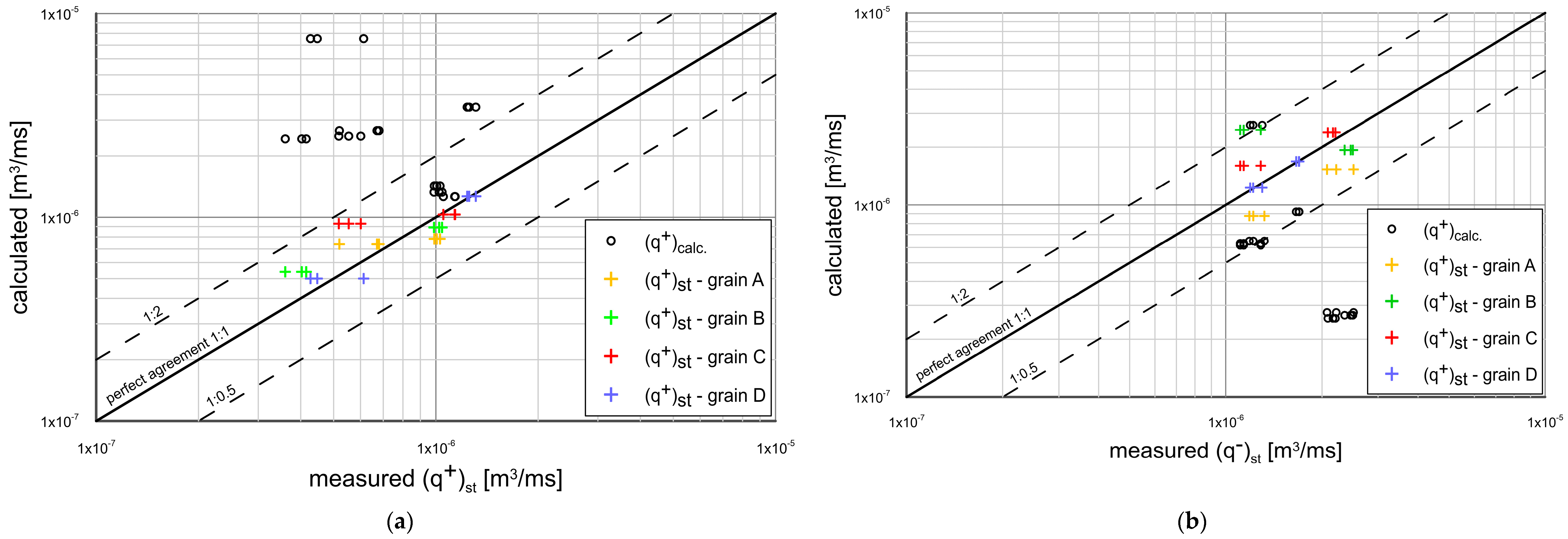
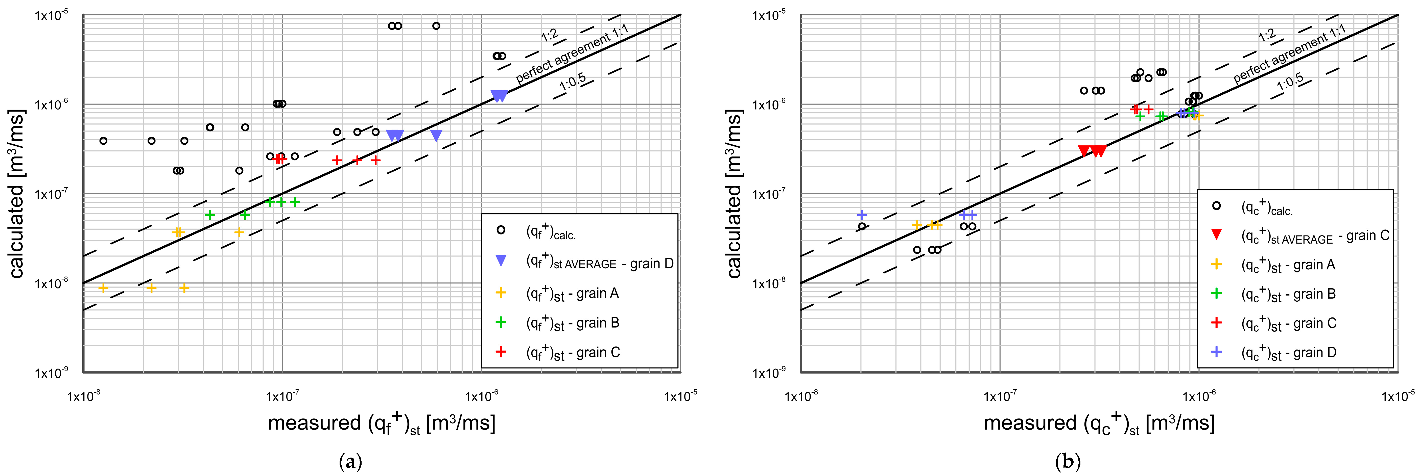
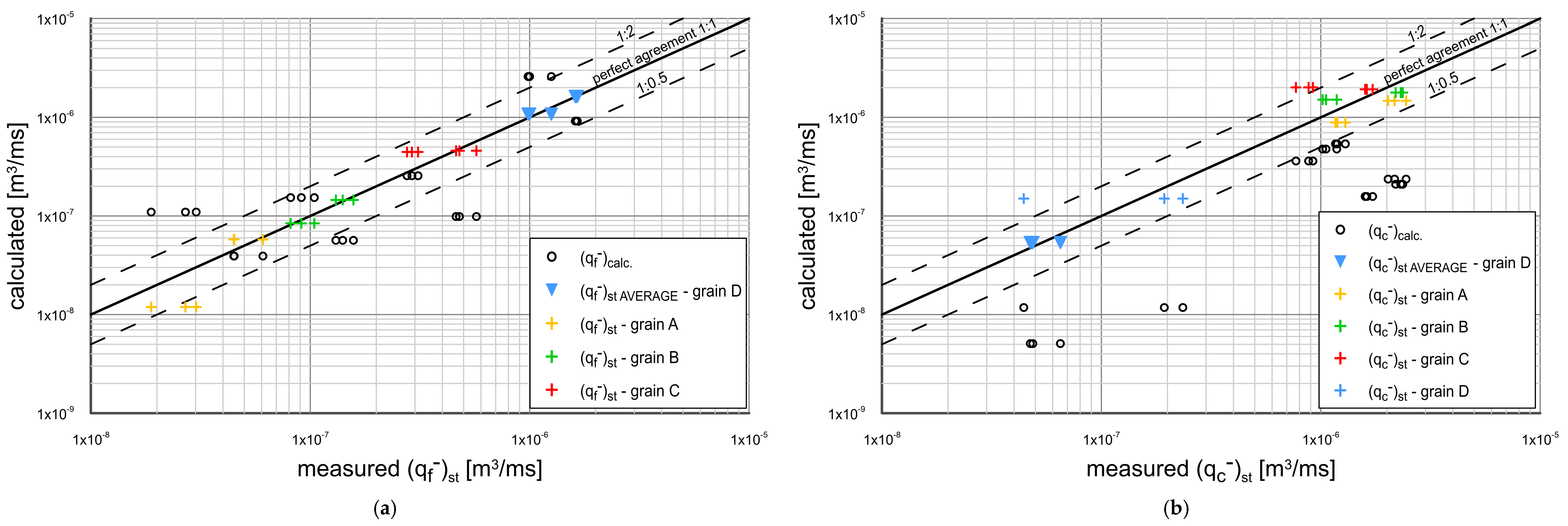
3.5. Calculated Sediment Transport versus Measurements

A comparison of the calculation results ${(q_{st}^{+/-})}_{calc.}$ carried out using the Kaczmarek et al. 2022 model according to Equations (5) ÷ (7) and the results of calculations $q_{st}^{+/-}$ carried out according to Equations (8) and (9) with the measurement results are presented in Figure 9a,b. The agreement was achieved within plus/minus a factor of 2 of the measurements, as shown by plotted agreement lines, and the results were compared separately for flows of fine and very fine fractions (Figure 10a) and coarse fractions in the crest phase (Figure 10b), as well as separately for flows of fine and very fine fractions (Figure 11a) and coarse fractions (Figure 11b) in the trough phase. The results presented in Figure 10 and Figure 11 suggest that very good agreement was obtained between the transport calculations ${(q_f^{+/-})}_{st}$ and ${(q_c^{+/-})}_{st}$ with the measured results. The agreement was achieved within plus/minus a factor of 2 of the measurements, as shown by the plotted agreement lines. As expected, the calculation results ${(q_{st}^{+/-})}_{calc.}$ deviated from the measurement results well beyond the agreement limits. In the case of fluxes in the crest phase ${(q_{st}^{+})}_{calc.}$ (Figure 9a), they significantly exceeded the measured results, while in the trough phase, the results ${(q_{st}^{-})}_{calc.}$ (Figure 9b) were significantly smaller than the measured results. This discordance was due to the presence of very fine and fine fractions and their influence on transport, which was not taken into account in the Kaczmarek et al. 2022 model. The above discordance was also very well visible in Figure 10a,b and Figure 11a,b, as the fluxes returning to the initial area in the trough phase caused the flux flow to significantly decrease ${(q_f^{+})}_{st}$ when entering the trap (Figure 10a). It is noteworthy that the prediction according to the Kaczmarek et al. 2022 model of coarse fractions entering the trap ${(q_c^{+})}_{calc.}$ (Figure 10b) also provided overestimated results, as it did not take into account the loss from the bottom and suspension of very fine fractions high above the bottom. As a result, the bottom became rougher, which caused a reduction in transport ${(q_c^{+})}_{st}$ in relation to ${(q_c^{+})}_{calc.} .$ In the trough phase (Figure 11a), both predictions ${(q_f^{-})}_{calc.}$ and ${(q_f^{-})}_{st}$ provided similar results, and agreement with the measurements was achieved within plus/minus a factor of 2 of the measurements, as it is shown by plotted agreement lines. The agreement of the results ${(q_f^{-})}_{st}$ with the measurements directly meant that the entire flux of fine fractions $q_{f3}^{-}$ flowed into the trap, feeding the total flux $q_{st}^{-}$. It is also worth noting the significant increase in coarse fractions in the flux ${(q_c^{-})}_{st}$. This increase is visible in Figure 11b; the prediction results ${(q_c^{-})}_{calc.}$ were strongly underestimated with respect to the measurements and flux values ${(q_c^{-})}_{st}$. The larger measurement and flux values ${(q_c^{-})}_{st}$ were caused by the influence of very fine fractions on the transport of coarse fractions by increasing their average value after the concentration depth. In summary, we assumed that if there were no very fine fractions in the bottom at all, but only fine fractions in the range of d_i < 0.20 mm, then Eq. ${(q_c^{+})}_{calc.}={(q_c^{+})}_{st}$ (Figure 10b) would apply, while the total flux $q_{st}^{+}={(q_f^{+})}_{st}+{(q_c^{+})}_{st}$ would be reduced only by the magnitude of fluxes of fine fractions $q_{f3}^{+}$ [36] (cf. Kaczmarek et al., 2022). For the trough phase, in such a situation the relations ${(q_c^{-})}_{st}={(q_c^{-})}_{calc.}$ and $q_{st}^{-}={(q^{-})}_{calc.}$ would be applied as the flux of fine fractions $q_{f3}^{-}$ flowed into the trap, feeding the total flux $q_{st}^{-}$.

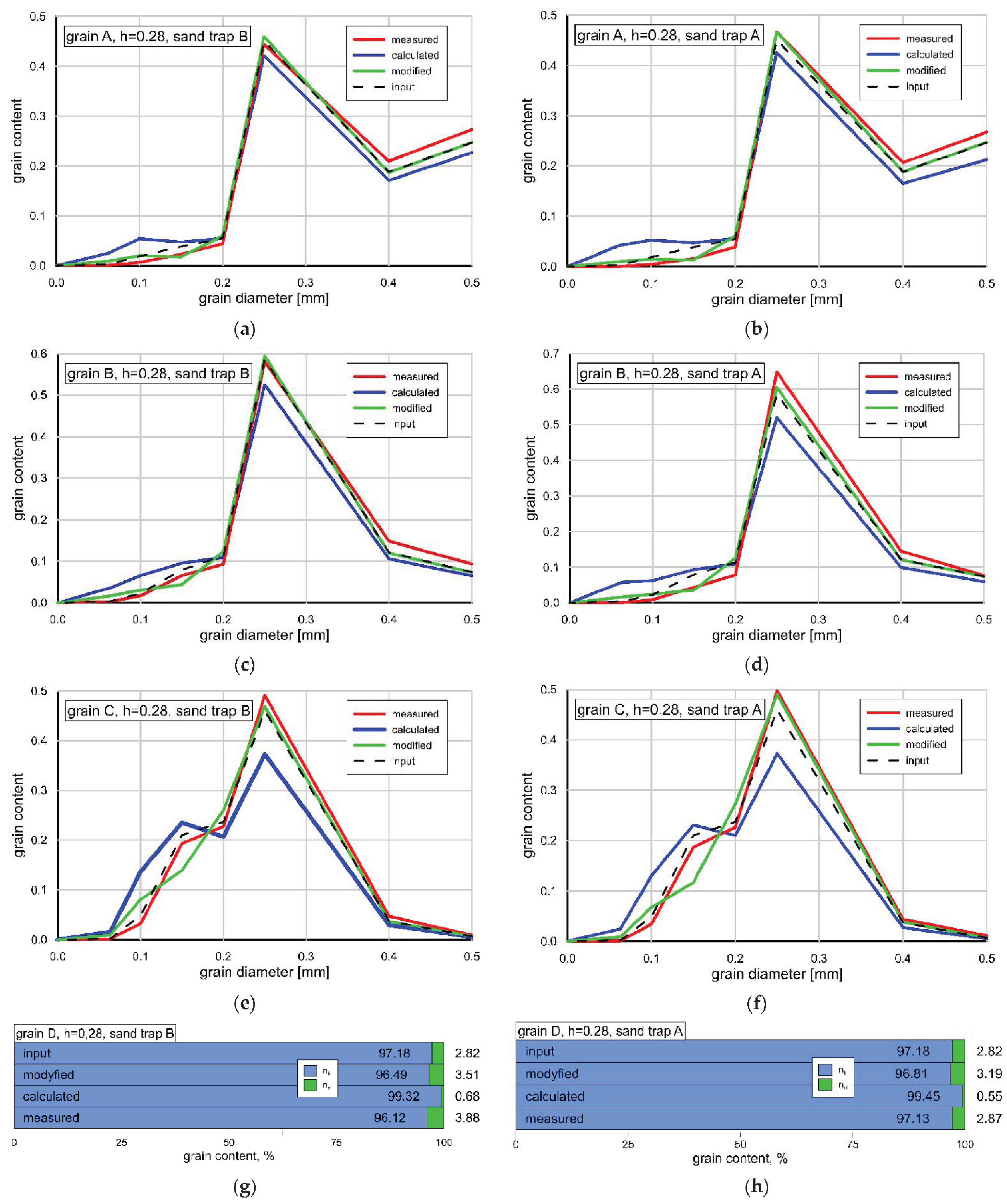
3.6. Calculated Grain Size Distributions versus Measurements

Figure 12 presents a comparison of the measured and calculated grain size distributions in the crest and trough phases for the four sands studied. Only the case for h = 0.28 m is presented here, as it is representative of both cases (h = 0.28 m and h = 0.36 m). The proportion of fine and very fine fractions ${(n_f^{+/-})}_{st}$ and coarse fractions ${(n_c^{+/-})}_{st}$ were calculated using Equations (19) and (20) for the crest phase and Equations (21) and (22) for the trough phase. For sands A, B, and C, a comparison of the measured and calculated grain size distributions of the i-th sediment fraction was made. However, for sand D, due to a large number of fine and very fine fractions (d₅₀ < 0.20 mm) and a very small amount of coarse fractions, only the calculated and measured total number of fine and very fine fractions $n_f^{+/-}={\displaystyle \sum }_{i=1}^{N_f}{n}_{fi}^{+/-}$ and the total amount of coarse fractions $n_c^{+/-}={\displaystyle \sum }_{i=N_f}^N{n}_{ci}^{+/-}$ were used. Calculations of the granulometric compositions were also carried out with the Kaczmarek et al. 2022 model, using Equations (17) and (18). Calculated granulometric compositions were compared with measurements of granulometric compositions of sediments caught in traps A and B for the trough and crest phases, respectively. Additionally, Figure 12 shows the measurement results of the initial grain size distribution with the proportion of fine and very fine fractions $n_{fi}$ and coarse fractions $n_{ci}$ of sediments in the control area.

It was noted that in all cases, the grain size distributions obtained using the three-layer model showed an overestimation of the content of fine and very fine fractions (d_i < 0.20 mm) and an underestimation of the content of coarse fractions (d_i ≥ 0.20 mm). This was due to the fact that the Kaczmarek et al. 2022 model did not take into account the effects of suspension of the finest fractions in the higher layer above the bottom and the effect of phase lags of the fine fractions, and as a result, the incomplete flux of fine and very fine fractions collected from the bottom in the crest phase fell entirely into trap B (Figure 12a,c,e,g). In the trough phase, the model of Kaczmarek et. al. 2022 did not take into account the effect of finest fractions on the increase in the coarse fraction content (Figure 12b,d,f,h) flowing into trap A. Therefore, it is worth emphasizing that the theoretical prediction, which took into account the correction coefficients resulting from the above effects, returned values similar to the measured ones.

Finally, it is worth noting that both in the crest phase (Figure 12a,c,e,g) measured and calculated with coefficients the proportion of fine and very fine fractions in sediments captured in trap B, and in the trough phase in trap A (Figure 12b,d,f,h), for all types of sands, the result was similar to the proportion measured in the input sediments. The contribution of these fractions, which was calculated using the Kaczmarek et al. 2022 model, showed significantly overestimated values. In contrast, the proportion of coarse fractions in both trap B and trap A for all sand types calculated using the Kaczmarek et al. 2022 model provided significantly underestimated values relative to both the input distribution and the measured and calculated magnitudes with correction factors.

4. Conclusions

The theoretical and experimental analyses of sediment fluxes in the wave crest and trough outgoing from the control area that were conducted in this paper allowed us to draw the following conclusions:

• Total sediment transport with very fine and fine (d_i < 0.20 mm) and coarse (d_i ≥ 0.20 mm) fractions, in both the crest and trough, consisted of the following components:

  ●

  Transport of outgoing sediment fluxes from the control area that were deposited in adjacent control areas in both directions. The movement of grains in these fluxes followed horizontal projection trajectories of different but equally probable lengths;

  ●

  Transport of fine sediment fluxes returning to the initial area in a suspended state. These fluxes were the result of phase lags between the water and sediment. Grains outgoing from the control area in the crest phase returned and were retained in this area. Then they flowed out in the trough as a flux that was deposited in the area adjacent to the trough side;

  ●

  Flux transports of very fine sediments returning to the initial area in the crest and trough phases in a suspended state—high above the bottom. These fluxes resulted from vertical sorting of the granulometrically heterogeneous sediment.

• An increase in the amount of very fine fractions in the return flow outgoing in the crest phase meant a loss in these fractions in the bottom, and thus an increase in the bottom roughness and grain movement resistance. As a result, the transport of coarse fractions outgoing in the flux from the control area and feeding the adjacent area decreased, and the transport of fine and very fine fractions decreased significantly due to the return of these fractions to the initial area. In the situation in which there were no very fine fractions in the bottom, only a loss in fine fractions was observed in the adjacent area due to the phase-lag effect.
• An increase in the amount of very fine fractions in the return flow outgoing in the trough phase caused an increase in the depth-averaged concentration of these fractions, and as a result, they formed an envelope around coarse grains, making the transport of these fractions easier, and significantly increasing the transport. In the case of a small amount of very fine fractions in the bottom, the above effect of these fractions on the transport of coarse grains was negligibly small, and the total flux outgoing in the trough was deposited in the adjacent area.
• The results of experimental investigations were compared with the results of theoretical analysis based on the three-layer model of Kaczmarek et al. 2022. As this model did not take into account the above-mentioned effects related to the presence of fine and very fine fractions, a modification of this model with the above-mentioned effects was proposed. Transport calculations were conducted separately for fluxes of very fine and fine fractions, coarse fractions, and total fractions outgoing in the crest and trough phase from the initial area and deposited in adjacent control areas. The consistency of the modified model with the measurements was achieved within plus/minus a factor of 2 of the measurements, as shown by plotted agreement lines. In addition, calculations of the granulometric distributions of sediment retained in the adjacent areas from the crest and trough were also carried out. Again, calculations were conducted separately for fine and very fine fractions, coarse fractions, and their sum. The calculated granulometric compositions were compared with measurements, and satisfactory agreement was obtained.
• Modification of the Kaczmarek et al. 2022 model was carried out based on four coefficients that corrected for fluxes of fine and very fine fractions and coarse fractions that fed adjacent control areas from the crest and trough. For sands with a relatively low content of fine fractions (d₅₀ ≥ 0.20 mm), it was possible to find a functional relationship of these coefficients with a coefficient of determination R² > 0.80. For sands with a dominant amount of fine and very fine fractions (d₅₀ < 0.20 mm), such a relationship could not be obtained, suggesting the need for further experimental studies in this area.
• An interpretation of the present laboratory experimental results in the natural situations could be easily made, as the free stream velocities were defined as the surface-wave-induced orbital velocity at the edge of the wave boundary layer, and the sediment transport was the result of the coexistence of wave motion asymmetry and compensatory return current. The present analysis of deposition from traps on the sides is highly recommended for engineering practices in coastal zone because the determination of sediment transport during the wave crest and wave trough is needed.

References

1. Ouillon, S. Why and How Do We Study Sediment Transport? Focus on Coastal Zones and Ongoing Methods. Water 2018, 10, 390. [Google Scholar] [CrossRef]
2. Ribberink, J.S. Bed-load transport for steady flows and unsteady oscillatory flows. Coast. Eng. 1998, 34, 59–82. [Google Scholar] [CrossRef]
3. Dibajnia, M.; Watanabe, A. Transport rate under irregular sheet flow conditions. Coast. Eng. 1998, 35, 167–183. [Google Scholar] [CrossRef]
4. Van Rijn, L.C. Unified View of Sediment Transport by Currents and Waves. I: Initiation of Motion, Bed Roughness, and Bed-Load Transport. J. Hydraul. Eng. 2007, 133, 649–667. [Google Scholar] [CrossRef] [Green Version]
5. Van Rijn, L.C. Unified View of Sediment Transport by Currents and Waves. II: Suspended Transport. J. Hydraul. Eng. 2007, 133, 668–689. [Google Scholar] [CrossRef]
6. Van Rijn, L.C. Unified View of Sediment Transport by Currents and Waves. III: Graded Beds. J. Hydraul. Eng. 2007, 133, 761–775. [Google Scholar] [CrossRef] [Green Version]
7. Van Rijn, L.C.; Walstra, D.J.R.; van Ormondt, M. Unified view of sediment transport by currents and waves. IV: Application of morphodynamic model. J. Hydraul. Eng. 2007, 133, 776–793. [Google Scholar] [CrossRef]
8. Kaczmarek, L.M.; Sawczyński, S.; Biegowski, J. Hydrodynamic Equilibrium for Sediment Transport and Bed Response to Wave Motion. Acta Geophys. 2015, 63, 486–513. [Google Scholar] [CrossRef] [Green Version]
9. Cannata, G.; Palleschi, F.; Iele, B.; Cioffi, F. A Three-Dimensional Numerical Study of Wave Induced Currents in the Cetraro Harbour Coastal Area (Italy). Water 2020, 12, 935. [Google Scholar] [CrossRef] [Green Version]
10. Zheng, J.H. Depth-dependent expression of obliquely incident wave induced radiation stress. Prog. Nat. Sci. 2007, 17, 1067–1073. [Google Scholar]
11. Zheng, J.; Mase, H.; Demirbilek, Z.; Lin, L. Implementation and evaluation of alternative wave breaking formulas in a coastal spectral wave model. Ocean Eng. 2008, 35, 1090–1101. [Google Scholar] [CrossRef]
12. Chen, X.W.; Zheng, J.H.; Zhang, C.; Yang, X. Evaluation of diffraction predictability in two phase averaged wave models. China Ocean. Eng. 2010, 24, 235–244. [Google Scholar]
13. Ribberink, J.S.; Al-Salem, A.A. Sediment transport in oscillatory boundary layers in cases of rippled beds and sheet flow. J. Geophys. Res. Earth Surf. 1994, 99, 12707–12727. [Google Scholar] [CrossRef]
14. Ribberink, J.S.; Chen, Z. Sediment transport of fine sand under asymmetric oscillatory flow. Delft Hydraul. Rep. H 1993, 840, part VII. [Google Scholar]
15. Dohmen-Janssen, C.; Kroekenstoel, D.F.; Hassan, W.N.; Ribberink, J.S. Phase lags in oscillatory sheet flow: Experiments and bed load modelling. Coast. Eng. 2002, 46, 61–87. [Google Scholar] [CrossRef]
16. Malarkey, J.; Davies, A.; Li, Z. A simple model of unsteady sheet-flow sediment transport. Coast. Eng. 2003, 48, 171–188. [Google Scholar] [CrossRef]
17. Van der Werf, J.J. Sand Transport over Rippled Beds in Oscillatory Flow. Ph.D. Thesis, University of Twente, Enschede, The Netherlands, 2006. [Google Scholar]
18. Briganti, R.; Dodd, N.; Incelli, G.; Kikkert, G. Numerical modelling of the flow and bed evolution of a single bore-driven swash event on a coarse sand beach. Coast. Eng. 2018, 142, 62–76. [Google Scholar] [CrossRef]
19. Hsu, T.-J.; Jenkins, J.T.; Liu, P.L.-F. On two-phase sediment transport: Sheet flow of massive particles. Proc. R. Soc. A Math. Phys. Eng. Sci. 2004, 460, 2223–2250. [Google Scholar] [CrossRef]
20. Da Silva, P.A.; Temperville, A.; Santos, F.S. Sand transport under combined current and wave conditions: A semi-unsteady, practical model. Coast. Eng. 2006, 53, 897–913. [Google Scholar] [CrossRef] [Green Version]
21. Cheng, Z.; Hsu, T.-J.; Calantoni, J. SedFoam: A multi-dimensional Eulerian two-phase model for sediment transport and its application to momentary bed failure. Coast. Eng. 2017, 119, 32–50. [Google Scholar] [CrossRef] [Green Version]
22. Ribberink, J.S.; Al-Salem, A.A. Sheet flow and suspension of sand in oscillatory boundary layers. Coast. Eng. 1995, 25, 205–225. [Google Scholar] [CrossRef]
23. O’Donoghue, T.; Wright, S. Concentrations in oscillatory sheet flow for well sorted and graded sands. Coast. Eng. 2004, 50, 117–138. [Google Scholar] [CrossRef]
24. O’Donoghue, T.; Wright, S. Flow tunnel measurements of velocities and sand flux in oscillatory sheet flow for well-sorted and graded sands. Coast. Eng. 2004, 51, 1163–1184. [Google Scholar] [CrossRef]
25. Rankin, K.L.; Hires, R.I. Laboratory measurement of bottom shear stress on a movable bed. J. Geophys. Res. Earth Surf. 2000, 105, 17011–17019. [Google Scholar] [CrossRef] [Green Version]
26. Jiang, Z.; Baldock, T.E. Direct bed shear measurements under loose bed swash flows. Coast. Eng. 2015, 100, 67–76. [Google Scholar] [CrossRef]
27. King, D.B. Studies in Oscillatory Flow Bedload Sediment Transport. Ph.D. Thesis, University of California, San Diego, CA, USA, 1991. [Google Scholar]
28. Hassan, W.N.; Ribberink, J.S. Transport processes of uniform and mixed sands in oscillatory sheet flow. Coast. Eng. 2005, 52, 745–770. [Google Scholar] [CrossRef]
29. Dohmen-Janssen, C.M.; Hanes, D.M. Sheet flow dynamics under monochromatic nonbreaking waves. J. Geophys. Res. Earth Surf. 2002, 107, 13-1–13-21. [Google Scholar] [CrossRef]
30. O’Donoghue, T.; Ribberink, J.S. Measurements of sheet flow transport in acceleration-skewed oscillatory flow and comparison with practical formulations. Coast. Eng. 2010, 57, 331–342. [Google Scholar] [CrossRef]
31. Schretlen, J.L.M. Sand Transport under Full-Scale Progressive Surface Waves. Ph.D. Thesis, University of Twente, Enschede, The Netherlands, 2012. [Google Scholar]
32. Cloin, B. Gradation Effects on Sediment Transport in Oscillatory Sheet-Flow. Master’s Thesis, Delft University of Technology (TU Delft), Delft, The Netherlands, 1998. [Google Scholar]
33. Xia, C.; Tian, H. A Quasi-Single-Phase Model for Debris Flows Incorporating Non-Newtonian Fluid Behavior. Water 2022, 14, 1369. [Google Scholar] [CrossRef]
34. Kaczmarek, L.M.; Biegowski, J.; Sobczak, Ł. Modeling of Sediment Transport in Steady Flow over Mobile Granular Bed. J. Hydraul. Eng. 2019, 145, 04019009. [Google Scholar] [CrossRef]
35. Kaczmarek, L.M. Numerical Calculations with a Multi-layer Model of Mixed Sand Transport Against Measurements in Wave Motion and Steady Flow. Rocz. Ochr. Srodowiska 2021, 23, 629–641. [Google Scholar] [CrossRef]
36. Kaczmarek, L.M.; Biegowski, J.; Sobczak, Ł. Modeling of Sediment Transport with a Mobile Mixed-Sand Bed in Wave Motion. J. Hydraul. Eng. 2022, 148, 04021054. [Google Scholar] [CrossRef]
37. Kaczmarek, L.M.; Sawczyński, S.; Biegowski, J. An Equilibrium Transport Formula for Modeling Sedimentation of Dredged Channels. Coast. Eng. J. 2017, 59, 1750015-1–1750015-35. [Google Scholar] [CrossRef]
38. Kaczmarek, L.M.; Biegowski, J.; Ostrowski, R. Modeling cross-shore intensive sand transport and changes of grain size dis-tribution versus field data. Costal Eng. 2004, 51, 501–529. [Google Scholar] [CrossRef]
39. Adrian, R.J. Particle imaging techniques for experimental fluid mechanics. Annu. Rev. Fluid Mech. 1991, 23, 261–304. [Google Scholar] [CrossRef]
40. Adrian, R.J. Twenty years of particle image velocimetry. Exp. Fluids 2005, 39, 159–169. [Google Scholar] [CrossRef]
41. Paprota, M. Experimental study on wave-current structure around a pneumatic breakwater. J. Hydro-Environ. Res. 2017, 17, 8–17. [Google Scholar] [CrossRef]
42. Paprota, M. Particle Image Velocimetry Measurements of Standing Wave Kinematics in Vicinity of a Rigid Vertical Wall. Instrum. Exp. Tech. 2019, 62, 277–282. [Google Scholar] [CrossRef]
43. Biegowski, J.; Paprota, M.; Sulisz, W. Particle Image Velocimetry Measurements of Flow Over an Ogee-Type Weir in a Hydraulic Flume. Int. J. Civ. Eng. 2020, 18, 1451–1462. [Google Scholar] [CrossRef]
44. Paprota, M. Experimental Study on Spatial Variation of Mass Transport Induced by Surface Waves Generated in a Finite-Depth Laboratory Flume. J. Phys. Oceanogr. 2020, 50, 3501–3511. [Google Scholar] [CrossRef]
45. Malarkey, J.; Davies, A. Free-stream velocity descriptions under waves with skewness and asymmetry. Coast. Eng. 2012, 68, 78–95. [Google Scholar] [CrossRef]
46. Stachurska, B.; Staroszczyk, R. Effect of surface wave skewness on near-bed sediment transport velocity. Cont. Shelf Res. 2021, 229, 104549. [Google Scholar] [CrossRef]
Figure 1. Vertical structure of the wave-induced progressive and reverse sediment fluxes.
Water 14 02397 g001
Figure 2. Sediment particle trajectories during the wave crest q s t + and trough q s t sediment transport.
Water 14 02397 g002
Figure 3. Experimental setup in a wave flume for measurements of wave-induced sediment transport: (a) side view of the wave flume with the sand box implemented; (b) side view of the wave flume.
Water 14 02397 g003
Figure 4. Close-up of the sediment section with position of gauges and sediment traps.
Water 14 02397 g004
Figure 5. PIV system layout and field-of-view position.
Water 14 02397 g005
Figure 6. Grain size distribution of quartz sands used in the experiment A: d50 = 0.38; B: d50 = 0.32; C: d50 = 0.25; D: d50 = 0.14.
Water 14 02397 g006
Figure 7. Characteristic records of the along-flume particle velocities.
Water 14 02397 g007
Figure 8. Plots of sediment flux correction factors: (a) fine fractions, crest phase; (b) coarse fractions, crest phase; (c) fine fractions, trough phase; (d) coarse fractions, trough phase.
Water 14 02397 g008
Figure 9. Comparison of calculated and measured transport during (a) the crest q + and (b) the trough q .
Water 14 02397 g009
Figure 10. Comparison of calculated and measured transport during the crest q+ in (a) fine fractions q f + and (b) coarse fractions q c + .
Water 14 02397 g010
Figure 11. Comparison of calculated and measured transport during the trough q- in (a) fine fractions q f and (b) coarse fractions q c .
Water 14 02397 g011
Figure 12. Comparison of calculated and measured grain size distributions in fine fractions and coarse fractions: (a) grain A—crest; (b) grain A—trough, (c) grain B—crest; (d) grain B—trough, (e) grain C—crest; (f) grain C—trough, (g) grain D—crest; (h) grain D—trough.
Water 14 02397 g012