Influence of Tubular Turbine Runaway for Back Pressure Power Generation on the Stability of Circulating Cooling Water System

Abstract

With the increasing maturity of tubular turbine power generation technology, an increasing number of industrial applications use it to recover the rich back pressure energy of a circulating cooling water system (CCWS). However, the influence of tubular turbine runaway on the stability of CCWS is still unclear. This work combines the one-dimensional (1D) method of characteristics (MOC) with the three-dimensional (3D) computational fluid dynamics (CFD), develops a 1D CCWS and 3D tubular turbine coupling simulation method, and simulates the runaway and runaway shutdown processes of tubular turbine under small flow rate condition and large flow rate condition in the real system. Results show that the main operating parameters of the system slightly change when the tubular turbine transitions from the steady state to the runaway condition. The runner’s radial force substantially increases in the runaway condition of the tubular turbine, and the phenomenon of violent oscillation is observed compared with the steady state. During the shutdown process of the tubular turbine runaway condition, the valves in parallel and series with the faulty turbine adopt a reasonable cooperative control strategy, which allows for a smooth recovery of the system operating pressure to the original steady state conditions.

1. Introduction

The circulating cooling water system (CCWS) is distinguished by its high energy and water consumption. This system is widely used in oil refining, the chemical industry, thermoelectricity, steel, food, and other fields, and its energy consumption accounts for approximately 20–30% of the total industrial production energy consumption [1]. The main energy-consuming equipment of the CCWS is the water pump and fan, among which the power consumption of the water pump can reach about 80% of the total energy consumption of the system [2]. When the installation elevation of the heat exchanger in the CCWS is larger than that of the cooling tower, a substantial quantity of power from the water pump must be consumed by the valves in the return water pipeline [3,4]. In the two cases in the literature [4], the turbine utilizes the abundant back pressure energy of the system to generate electricity, which can recover 36.8% and 39.1% of the pump power consumption.

According to statistics, the surplus back pressure of the CCWS is typically 5–30 m [5], which is a low head residual energy system. The tubular turbine is suitable for low water head and large flow rate scenarios [6], and the water head range is typically 2–25 m. This turbine is more suitable for the CCWS residual energy power generation than the Francis [7] and axial flow [8] turbines. In this work, the tubular water turbine is arranged in the upper tower pipeline of the cooling tower in the CCWS, and the water turbine replaces the decompression effect of the upper tower valve of the cooling tower, as shown in Figure 1.

The tubular turbine has a short flow channel, and the water flow in the flow channel is basically in a straight-in and straight-out state, which reduces the hydraulic loss and impact caused by the turning of the water flow, so it has high hydraulic efficiency and stability during a normal operation. However, significant pressure pulsation and vibration problems occur during the runaway process after the unit failure and grid disconnection due to the low inertia constant of the tubular turbine [9], which can result in safety accidents. In 2004, the Feilaixia Hydropower Station [10] 2# unit entered the runaway state due to electrical failure, and the unit vibration exceeded the standard, resulting in the fracture of the steel wire rope of the guide vane sensor. In 2013, shortly after the Xiaoxuan hydropower station [11] began operation, the 2# unit reached a runaway state due to a broken guide vane pin during shutdown, and the unit had abnormal problems of operating sound, vibration, and ferry. Then, the unit was able to smoothly shut down by reconnecting to the grid and shutting the outlet. At present, research on the runaway characteristics of tubular turbines in pipe network systems, especially in CCWS, is almost non-existent despite studies on the runaway process characteristics of tubular turbines [12,13]. Whether the fault runaway of the tubular turbine will cause substantial water hammer [14] to the CCWS is not clear. In addition, unlike the previous shutdown mode of a tubular turbine in a runaway state, this work realizes the shutdown by controlling the valves in parallel and series with the failed turbine. Whether this shutdown mode will bring new water hammer to the CCWS is not clear, and the better shutdown strategy remains to be discussed. Therefore, the runaway and runaway shutdown processes of tubular turbines in the CCWS must be explored.

In terms of research methods, numerical simulation is an effective tool to study the runaway process of hydro turbines. The reason is that the cost of building a system model test is expensive, and the runaway test on a real system on site cannot be implemented due to the lack of safe operating conditions. Conventional numerical simulation methods are divided into one-dimensional (1D) and three-dimensional (3D). The 1D method of characteristics (MOC) [15,16,17] is not only theoretically rigorous but also easy to program and implement. This method has also become the most commonly used method for solving 1D transient flows. In addition, 3D computational fluid dynamics (CFD) based on Navier–Stokes (N–S) equations and turbulence models have been widely used with the rapid development of CFD [7,8,9,12,13,18]. The advantages of the 3D numerical method are that it can more accurately reflect the 3D characteristics of the flow field and avoid the error caused by many conditional assumptions and simplification in the 1D analysis with the 1D numerical method. However, the 3D numerical method cannot meet the computational requirements for the problem studied in this work. The reason is that if only the 3D modeling of the tubular turbine is carried out, then calculation will be impossible because of the absence of an accurate dynamic boundary condition for the runaway process of turbines. If a 3D model is also built for a large pipe network system, then the process will take a long time, ranging from a few months to several years, due to the excessive amount of calculation. At present, this mechanism does not have the application conditions.

In recent years, using 1D and 3D coupled algorithms to analyze the transient flow in large-scale pipe network systems with a complex hydraulic machinery has become a new trend, combining the advantages and disadvantages of the two scale simulation methods [19,20,21,22,23]. Yang et al. [19] developed a coupled simulation program of 1D MOC and 3D CFD and verified its calculation accuracy through the pipeline-valve-pump experimental system. Li et al. [20] established the coupling algorithm between a pipeline 1D underwater acoustic model and a unit 3D CFD when studying the transient process of a pump turbine. Liu et al. [21] established the coupling algorithm between a pipeline 1D MOC and a unit 3D CFD and proved that the 1D–3D coupling method is feasible for evaluating the transient risk of a pumped storage power station.

In summary, the effect of tubular turbine runaway on the stability of CCWS must be studied. In this work, the CCWS 1D MOC and the 3D CFD coupling simulation method of the tubular turbine are developed. On this basis, the runaway and runaway shutdown processes of tubular turbines in the actual system are analyzed. This work not only has a certain role in promoting the engineering application of the recovery of CCWS rich back pressure energy by the tubular turbine but also has certain guiding significance for the establishment of the protection and control strategy of the tubular turbine in the system.

2. Numerical Calculation Method

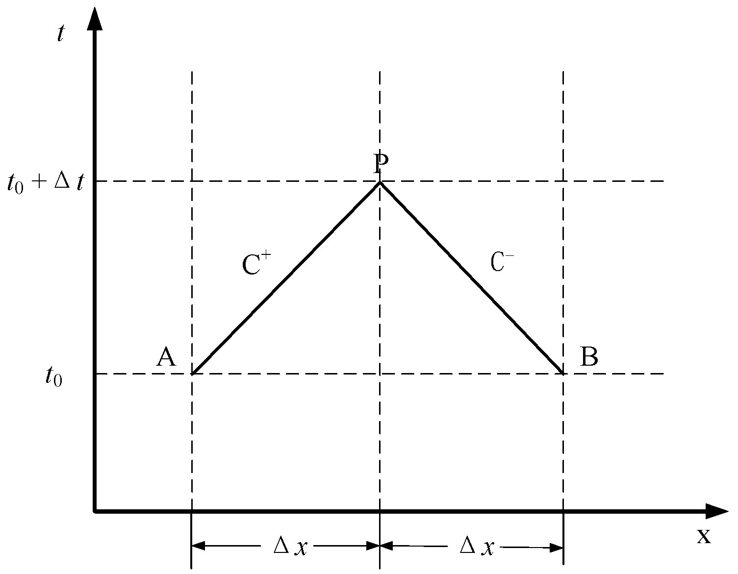
2.1. CCWS 1D MOC Method

The motion and continuity equations describing the 1D unsteady flow in CCWS are quasi-linear hyperbolic partial differential equations, and the analytical solutions are obtained by using the MOC in this work.

Equations (1) and (2) are characteristic equations represented by C⁺ and C⁻, which are explained by Figure 2. Variable Δx is the length of the pipeline that the water hammer travels at time Δt.

C⁺ equations:

$$H_{Pi}=C_P-B{Q}_{Pi},$$

(1)

C⁻ equations:

$$H_{Pi}=C_M+B{Q}_{Pi},$$

(2)

$$C_P=H_{i-1}+B{Q}_{i-1}-R{Q}_{i-1}\left|Q_{i-1}\right|,$$

(3)

$$C_M=H_{i+1}-B{Q}_{i+1}+R{Q}_{i+1}\left|Q_{i+1}\right|.$$

(4)

H and v of points A and B at time t₀ are known, and the above equations can be simultaneously solved to determine the H_p and v_p of intersection point P of lines C⁺ and C⁻ at time t₀ + Δt. Then, the calculation pipe section is divided into N sections, according to the calculation accuracy requirements. The total number of pipe nodes is N + 1. Each node is represented by i, the space step Δx = L/N, and the time step Δt = Δx/a. Let $B=a/gA$, and $R=f\Delta x/2gD{A}^2$. The characteristic equation can be expressed as the following form. Finally, a program is compiled to carry out numerical simulation calculations in combination with the initial conditions and boundary conditions of the boundary points in the pipeline system based on the characteristic equations.

The pressure of the cooling water entering the system pipe network is determined by the liquid level of the sump, and it is considered constant during the transient process. The pressure of the cooling water flowing out of the pipe network into the cooling tower can be approximated to atmospheric pressure. The boundary conditions to be established in this model also include the upstream pump station, the joint of the reducing pipe, the joint of the reducer, and the simplified resistance element of the heat exchanger network. Given the space limitations, this work only establishes the boundary conditions of the running water pump. Take the solution as an example. When the pumping station is in a normal operation, the boundary conditions can be expressed in the form of Figure 3, and the Q–H characteristic curve of the centrifugal pumps in parallel operation can be fitted to a quadratic polynomial.

$$H=a_1+a_{2}Q+a_3{Q}^2,$$

(5)

where H is the head of the pump station; Q is the total flow rate of the pump station; and a₁, a₂, and a₃ are constants related to the combination of the pumps.

Let the inlet node of the pump station be s and the outlet node be d. The friction loss ΔH in the pump station can be approximated as a constant.

The C⁻ equation of the outlet pressure head of the pumping station is as follows:

$$H_{Pd}=C_M+B_2{Q}_{Pd},$$

(6)

The flow rate continuity equation is expressed as follows:

$$Q_P=Q_{Ps}=Q_{Pd},$$

(7)

The pressure balance equation is as follows:

$$H_{Pd}=H_{Ps}+H+\Delta H,$$

(8)

Arranging and solving Equations (5)–(8) in parallel yield:

$$Q_P=\frac{1}{2a_3}\left[\left(B_2-a_2\right)-\sqrt{{\left(a_2-B_2\right)}^2-4a_3\left(a_1+H_{Ps}-C_M-\Delta H\right)}\right].$$

(9)

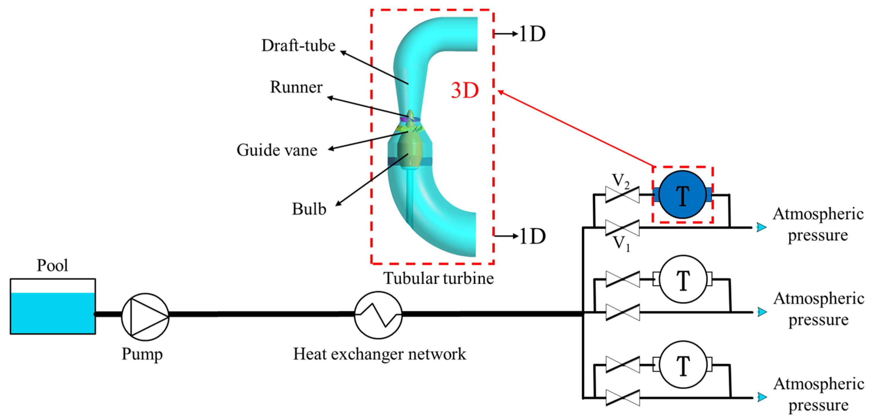
2.2. 3D CFD Method for a Tubular Turbine

The internal flow of the tubular turbine satisfies the law of conservation of mass, the law of conservation of momentum, and the law of conservation of energy. In this study, the flow in the turbine is approximated as an incompressible 3D viscous unsteady turbulent flow. Thus, the N–S equations can be written as follows:

$$\{\begin{array}{l}\frac{\partial u_j}{\partial x_j}=0\\ \frac{\partial u_i}{\partial t}+u_j\frac{\partial u_i}{\partial x_j}=-\frac{1}{\rho }\frac{\partial p}{\partial x_j}+\nu \frac{{\partial }^2{u}_i}{\partial x_i\partial x_j}+f_i\end{array},$$

(10)

where u_i is the instantaneous velocity, p is the instantaneous pressure, ρ is the density, $\nu$ is the kinematic viscosity coefficient of the water molecules, and f_i is the body force.

However, the nonlinear transport term in the N–S equation makes it nearly impossible to obtain an analytical solution to the N–S equation. The discrete methods of the governing equations include the finite difference method [24], finite element method [25], and finite volume method [26]. The finite volume method has better conservation and computational efficiency compared with the other two discretization methods. Thus, this method is used for the discretization of the governing equations in this work. In addition, Equation system (10) is not complete. Since the SST k-ω turbulence model can accurately predict the separation amount without over predicting the eddy viscosity, and the prediction of the reverse pressure gradient and the near wall flow has been significantly improved. Therefore, this work adopts the SST k–ω two-equation turbulence model [20,27] to complete Equation (10). SST k–ω combines the modeling ideas of the standard k–ε and k–ω models. The k–ω model is used for the near wall surface, and the standard k–ε model is utilized for the mainstream area. The eddy viscosity coefficient μ_t is defined as the turbulent kinetic energy k, and the Function of special loss rate ω, k, and ω are solved by using two transport equations.

The mathematical expression of the SST k–ω two-equation turbulence model is as follows:

$$\frac{\partial }{\partial t}(\rho k)+\frac{\partial }{\partial x_j}(\rho u_{j}k)=\frac{\partial }{\partial x_j}((\mu +\frac{{\mu }_t}{{\sigma }_{k3}})\frac{\partial k}{\partial x_j})+P_k-{\beta }^{\prime }\rho k\omega ,$$

(11)

$$\frac{\partial }{\partial t}(\rho \omega )+\frac{\partial }{\partial x_j}(\rho u_j\omega )=\frac{\partial }{\partial x_j}((\mu +\frac{{\mu }_t}{{\sigma }_{\omega 3}})\frac{\partial \omega }{\partial x_j})+\frac{2\rho {\sigma }_{\omega 2}(1-F_1)}{\omega }\frac{\partial k}{\partial x_i}\frac{\partial \omega }{\partial x_i}+{\alpha }_3\frac{\omega }{k}{P}_k-{\beta }_{{}_0}\rho {\omega }^2,$$

(12)

where y is the distance to the wall, ${\beta }^{\prime }=0.090$, ${\alpha }_1=0.5532$, ${\beta }_1=0.0750$, ${\sigma }_{k1}=1.000$, ${\sigma }_{\omega 1}=2.000$, ${\alpha }_2=0.4404$, ${\beta }_2=0.0828$, ${\sigma }_{k2}=1.000$, and ${\sigma }_{\omega 2}=1/0.865$.

The eddy viscosity μ_t is expressed as follows:

$${\mu }_t=\frac{a_{1}k}{\max (a_1\omega ,S{F}_2)},$$

(13)

where a₁ = 0.310, k is the turbulent kinetic energy, and ω is the turbulent frequency.

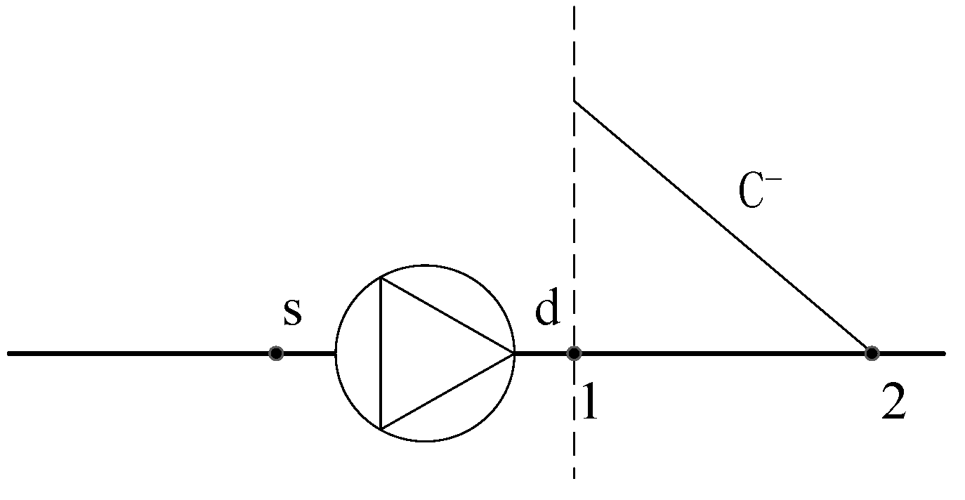
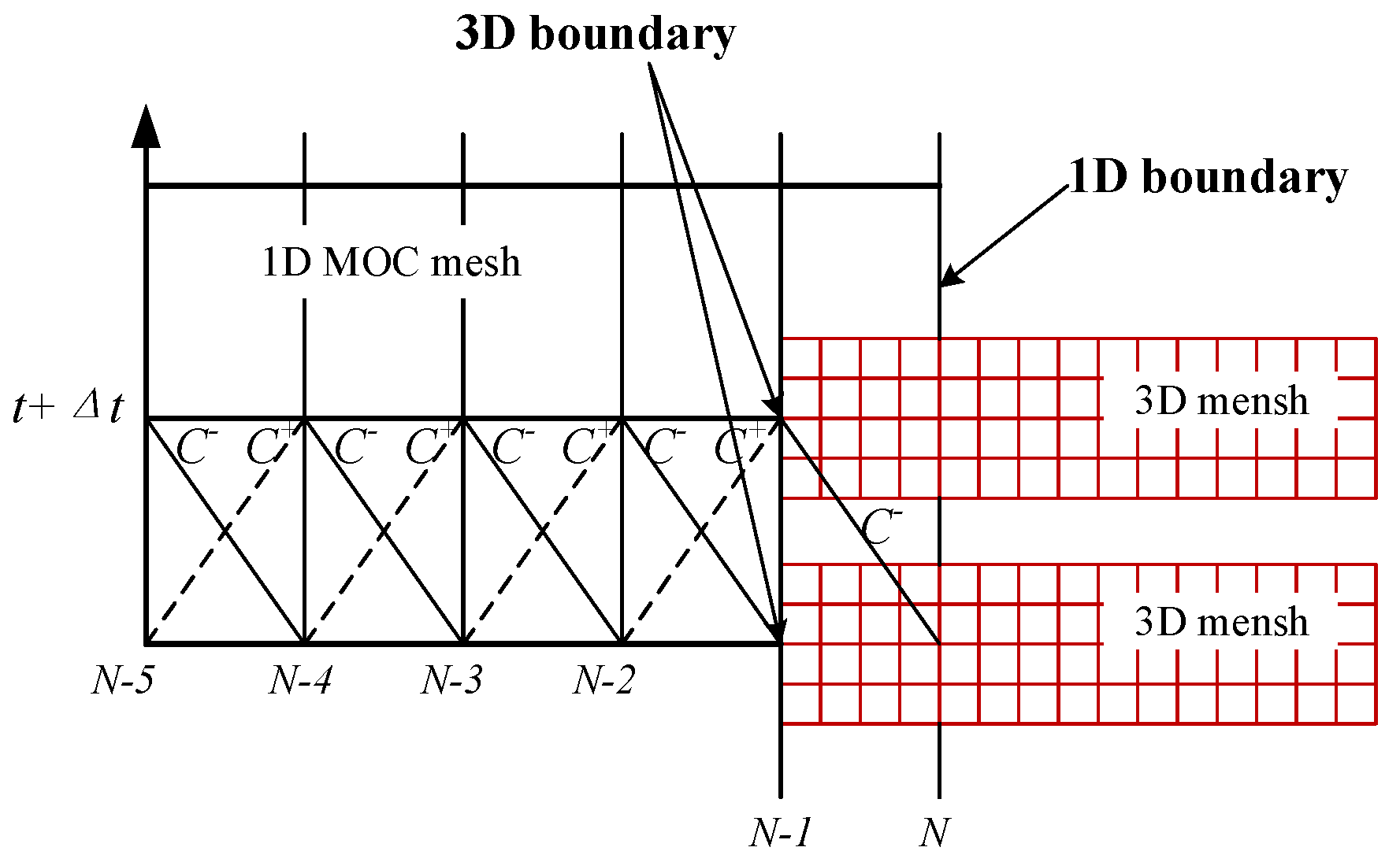
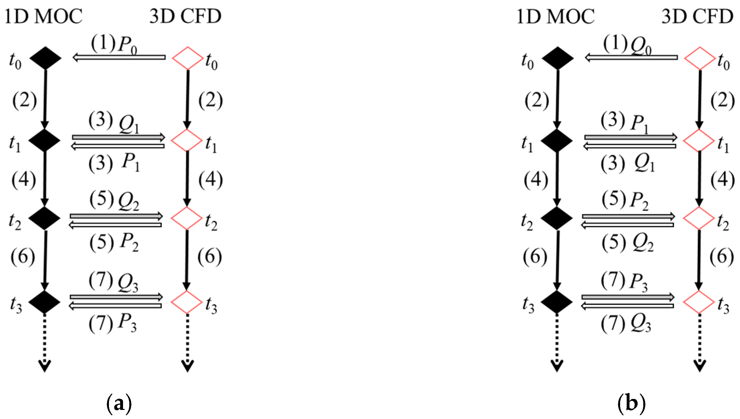
2.3. 1D MOC–3D CFD Coupled Simulation Method

In this work, a coupled simulation method of 1D MOC and 3D CFD is proposed, and the boundary conditions between the 1D and 3D domains are coupled by the method of partial mesh overlap [28,29], as shown in Figure 4.

Given that the 1D model is relatively fast to calculate, the time step of 1D MOC is subject to the time step of 3D CFD. 1D MOC part is calculated by the software Flowmaster, and 3D CFD part is calculated by the software ANSYS Fluent. Although the two dimensions are solved separately in the data exchange process, the calculation results need to be transmitted to each other at the two interfaces of the turbine inlet and outlet in every iteration step. The 1D MOC code completes one step of the iteration, and it sends the data to the 3D CFD code, which uses it in its own iteration. In general, the pressure or flow rate transmitted from 3D to 1D is the average value of the two interfaces. The iterative computations for the two dimensions continue separately until both dimensions converge. Figure 5 shows the data transfer mechanism of the turbine inlet and outlet coupling interface:

To simulate the runaway process of the turbine in the 3D calculation domain, we use the secondary development interface of ANSYS Fluent software and C language to write its identifiable UDF to control and calculate certain parameters, such as speed and torque, in the runaway process. This program controls the turbine torque and rotational speed according to the rotational balance equation

The rotational motion equation of the hydro-generator set is as follows:

$$M_t-M_g=J\frac{dn}{dt}$$

(14)

where M_t is the resultant moment acting on the runner, M_g is the load torque, n is the runner rotational speed, and J is the moment of inertia. Friction is ignored in this work, because friction is relatively small, and ignoring it will not significantly affect the speed calculation results. The tubular turbine generator unit is small because of the moment of inertia. The total inertia moment of the unit is the sum of the additional inertia moment of generator ($J_1$), water turbine ($J_2$), and water body ($J_3$). The calculation method of the total moment of inertia is shown as Equation (15).

$$J^2=J_1^2+J_2^2+J_3^{{}^2}.$$

(15)

According to the real machine measurement and calculation, the total moment of inertia is obtained as 8 kg m².

Given that the turbine does not carry a load after an accidental power failure, M_g = 0, the rotational angular velocity of the runner at any time is as follows:

$$n^{i+1}=n^i+\frac{M_t{}^i}{J}\times \Delta t,$$

(16)

where M_tⁱ is the runner torque at the i moment; nⁱ and n^{i + 1} are the rotational speed at the i moment and after a time step, respectively; and Δt is the time step.

The coupling algorithm is used to simulate the runaway process of the turbine, and the specific steps are as follows:

The initial boundary conditions of the 1D model and the 3D model are obtained through field testing. The 1D model adopts the pressure boundary. Meanwhile, the 3D model adopts the inlet mass flow rate and outlet pressure boundary;

Before the calculation of the runaway process of the turbine, the steady state calculation is carried out under the initial boundary conditions of the 3D model. Then, the flow field of the turbine under steady state conditions is determined, and it is used as the initial file of the 3D model in the transient calculation;

Unsteady calculation is performed on the coupled model. Before starting the calculation of the transient process, unsteady calculation is performed on the steady state of the coupled model for a certain period of time to ensure the convergence in the transient process. The working parameters of water moment, angular velocity, and runner axial force of the turbine runner under steady state conditions are obtained through the self-compiled plug-in. In each time step, 1D MOC and 3D CFD are calculated separately, and the calculation results are transmitted to each other through the interface;

At the beginning of the runaway process, the rotation speed of the next time step is calculated according to the custom function prepared by Equation (16). In this way, the rotation speed of the runner is updated in every time step, which is sequentially iterated to obtain the instantaneous working parameters, thus realizing the whole calculation process of the runaway transient;

The change process of the water moment at the shaft end of the turbine is monitored during the calculation process, and whether the water moment at the shaft end is close to zero is examined. Otherwise, the iterative calculation is continued, or it is terminated.

3. Computational Model and Reliability Verification

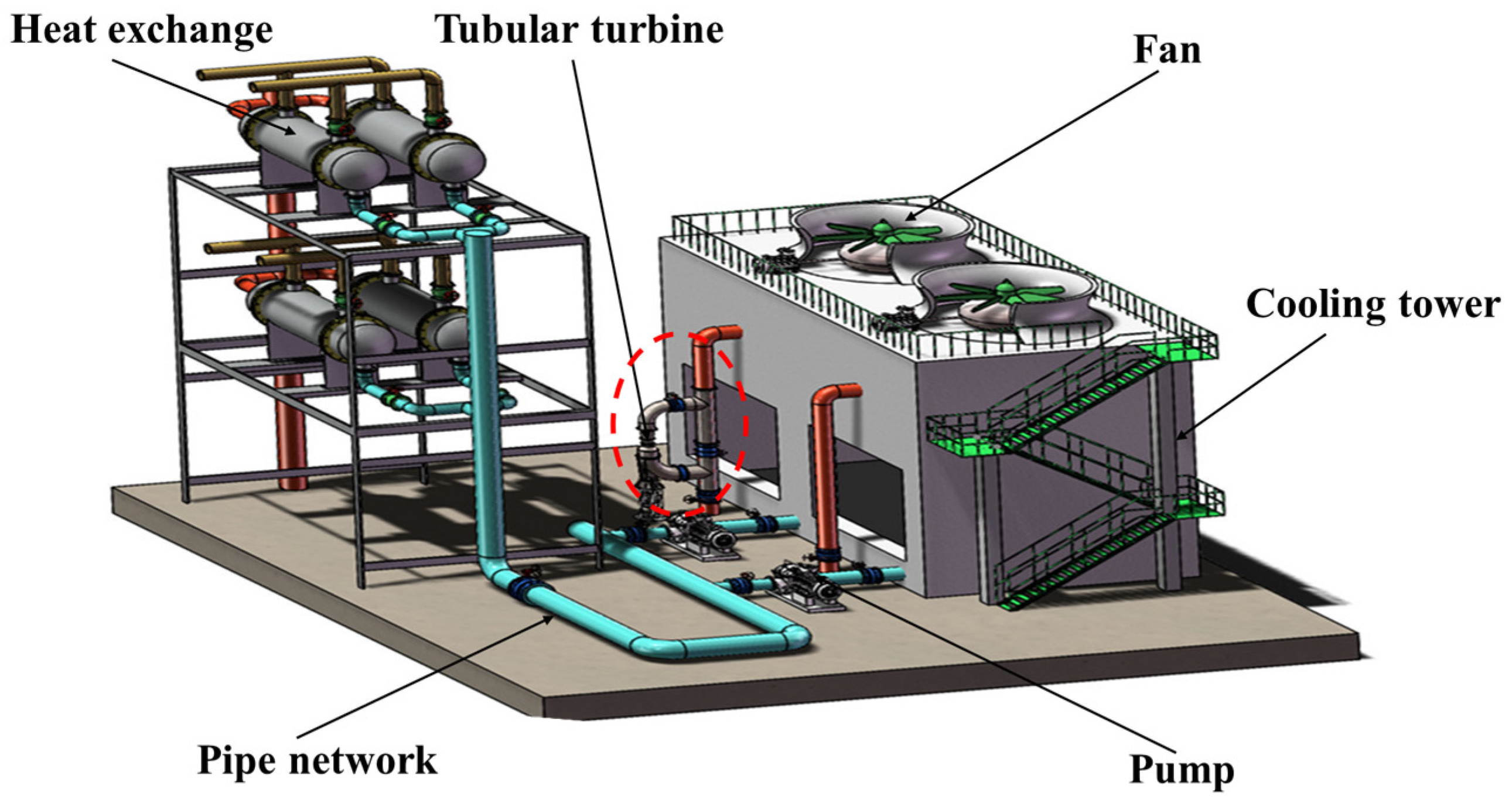
3.1. System Coupling Model

In this study, the actual circulating cooling water system with back pressure power generation was investigated. The system under study is equipped with three counter-flow cooling towers, and the designed cooling capacity of a single cooling tower is 4500 m³/h. Three fixed-blade tubular turbines were used on site to replace the original upper tower valve, and the extra back pressure of the system was used to generate electricity. Considering the investment cost, operation life and power generation of the hydraulic turbine, the annual income of the system after the optimization and transformation of residual pressure power generation is about 400,000 $. It can be seen that using the residual voltage of the system to generate electricity has high economic benefits. The specific parameters of the turbine are shown in

Table 1. Geometric parameters of the bulb turbine.

Name	Date	Unit
Propeller blade	5	Piece
Vane	12	Piece
Blade opening	21	°
Guide vane opening	76	°
Runner speed	1500	r/min
Rotational inertia	8	Kg m2
Runner diameter	430	mm
Bulb diameter	450	mm
Inlet diameter	900	mm
Outlet diameter	800	mm

.

In this work, all the components of the 3D turbine model are divided into hexahedral structured meshes. This work selects four sets of grids for grid independence verification, and the number of grids ranges from 2.98 million to 5.33 million. The results are shown in

Table 2. Mesh independence result.

Number of Mesh (Million)	Head (m)	Efficiency (%)
298	19.18	91.09
382	19.35	91.14
456	19.36	91.15
533	19.36	91.15

. Considering the calculation accuracy and calculation time allowance, 4.56 million grids were finally selected for the numerical simulation calculation.

Furthermore, three time steps (1.1 × 10⁻⁴, 2.2 × 10⁻⁴, and 3.3 × 10⁻⁴ s) were used to verify the time-step independence of the 3D model of the hydraulic turbine. The three time steps correspond to the time required for the runner to rotate 1°, 2°, and 3° at the design speed. The pressure calculation results of a certain measuring point in the runner domain under the three time steps are shown in Figure 6. Considering the calculation accuracy and calculation speed, the final time step is 2.2 × 10⁻⁴ s. Where T_n is the time required for the runner to rotate for one revolution.

In this work, the 3D model of the hydraulic turbine has been calculated under several working conditions to verify the reliability of the calculation of the 3D model of the turbine. The model tests the real situation of the turbine head and efficiency under different flow rate conditions by adjusting the valves in the heat exchanger network. The head (H) and efficiency (η) of the on-site turbine are obtained according to Equation (17).

$$\{\begin{array}{l}H=\frac{P_{\mathrm{in}}-P_{\mathrm{out}}}{\rho g}+\Delta h\\ \eta =\frac{N_{\mathrm{m}}}{\rho gQH{\eta }_{\mathrm{m}}}\end{array}$$

(17)

where Q is the operating flow of the turbine, which can be read through the flowmeter; P_in and P_out are the inlet and outlet pressure of the turbine respectively, which can be read through the pressure gauge; Δh is the height difference of inlet and outlet pressure gauges; N_m is the instantaneous generating capacity of the turbine, which can be read by the electricity meter; η_m is the generator efficiency, which can be obtained according to the parameters provided by the manufacturer.

The results are compared with the experimental values, as shown in Figure 7. The numerical simulation is consistent with the distribution law of the experimental values. The optimal flow rate (Q_BEP) is 4100 m³/h. The numerical simulation and experimental water heads under the optimal working conditions are 19.6 and 18.6, and the efficiencies are 91.2% and 88.3%, respectively; thus, the errors of the water head and efficiency are 5.1% and 3.2%, respectively. The simulated values of the 3D model are in good agreement with the experimental values, thereby accurately reflecting the external characteristics of the turbine. In addition, it can be found that the test results are slightly smaller than the numerical results, mainly because only hydraulic efficiency is considered in the numerical simulation.

The runaway and shutdown transient processes studied in this work are as follows: when three turbines operate in parallel under the same working conditions to generate electricity, one of the turbines fails and powers off to reach the runaway state. Then, remote control valves V₁ and V₂ shut off the runaway turbine. A 3D model is established for a hydraulic turbine, the other two parallel turbine branches belong to 1D simulation area, and the water supply network is simplified based on the hydraulic equivalence theory [28,30]. The coupled model is shown in Figure 8. The figure demonstrates that when the turbine unit is in the normal operation, valve V₁ is closed, and valve V₂ is opened. When the turbine unit is disconnected from the system, valve V₂ is closed, and valve V₁ is opened.

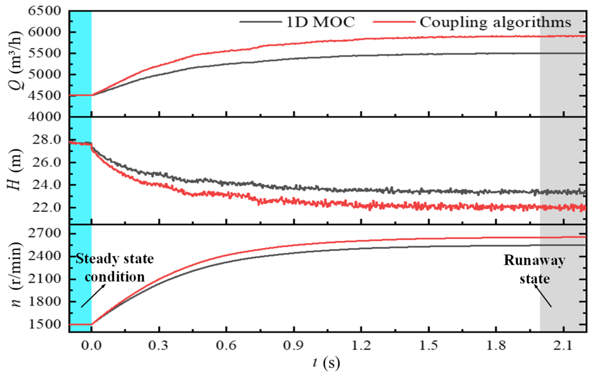
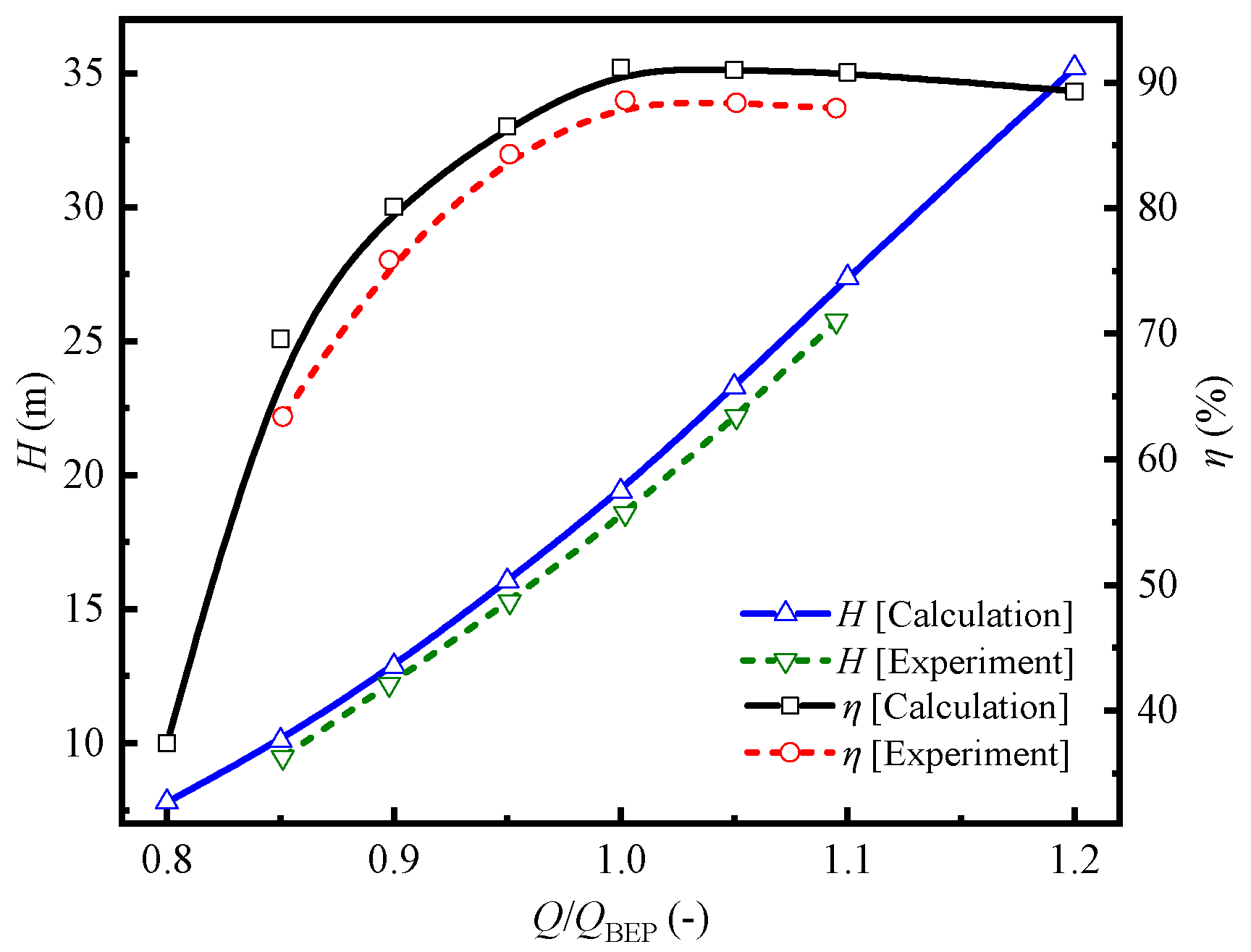
3.2. Comparative Analysis of the Coupling Algorithm and 1D MOC Calculation Results

In the coupling calculation, the position of the coupling interface of the turbine inlet and outlet takes the pressure and flow rate as the parameters for data transmission, and the accuracy of the data transmission is ensured through iteration. The independent 1D MOC calculation results care compared to further verify the reliability of the coupled simulation method. The comparison variables include the flow rate, head, and speed of the runaway turbine, and the steady state flow rate before the runaway of the turbine is 1.1Q_BEP. During calculation, the static pressure of the sump is 19,600 Pa and the local atmospheric pressure is 101,325 Pa. The comparison results are shown in Figure 9. The results of the two methods show good consistency. Moreover, the flow rate, head, and rotational speed of the turbine are basically stable under the runaway state of the turbine.

Table 3. Comparison of the main parameters of the turbine runaway state.

Runaway State	Q (m3/h)	H (m)	n (r/min)
1D MOC	5492	23.4	2539
Coupling algorithm	5893	22.1	2645
Error rate (%)	7.3	5.6	4.2

shows the comparison of turbine flow rate, head, and speed in the runaway state. The errors of the three parameters calculated by the two methods are 7.3%, 5.6%, and 4.2%. The relative error between the 1D MOC method and the coupling algorithm used in the run-away transient calculation is within the conventional range, and the reliability of the coupling algorithm can be considered to meet the requirements. In comparison with the 1D MOC method, this algorithm is more suitable for evaluating the pressure pulsation and the force of the runner of the turbine during the run-away process.

4. Results and Discussion

The system flow rate is affected by external factors, such as production load and ambient wet bulb temperature [2,31]. The turbine needs to operate within a certain flow rate range, and the runaway process calculation needs to consider the maximum and minimum flow rate conditions. According to historical operating data, the operating flow rate of the turbine is determined to be between 0.85Q_BEP and 1.1Q_BEP. This work conducts a coupled simulation of the turbine runaway process when the initial steady state flow rates (abbreviated as initial flow rate) are 0.85Q_BEP and 1.1Q_BEP to comprehensively analyze the runaway and runaway shutdown process of the turbine.

4.1. Analysis of the Influence of the Runaway Process of the Turbine on the Main Parameters of the System

To more intuitively analyze the variation law of the main operating parameters of CCWS with time during the runaway process, three dimensionless coefficients are introduced, namely, the system return pressure relative value, the relative value of the system flow rate, and the turbine flow rate in parallel with the runaway turbine. The flow rate of two parallel turbines in normal operation is almost the same. The relative values, denoted as P_out,rel, Q_total,rel, and Q_par,rel, represent the ratio of the instantaneous value of each parameter to the initial value before escape, as shown in Equation (18)

$$\{\begin{array}{l}{P}_{\mathrm{out},\mathrm{rel}}=P_{\mathrm{out},t}/P_{\mathrm{out},0}\\ Q_{\mathrm{total},\mathrm{rel}}=Q_{\mathrm{total}}/Q_{\mathrm{total},0}\\ Q_{\mathrm{par},\mathrm{rel}}=Q_{\mathrm{par},t}/Q_{\mathrm{par},0}\end{array},$$

(18)

where subscript t represents the instantaneous value, and subscript 0 denotes the initial value.

The runaway of the turbine will affect the pressure of the system pipe network. Considering that the turbine is set on the system return water tower pipeline, the pressure fluctuation will first be reflected in the system return water pressure. Accordingly, this work takes the variation trend of the system return water pressure as an example to illustrate the influence of the runaway process on the system pressure, as shown in Figure 10a. After the turbine runaway occurs in the system, the return water pressure of the system will gradually decrease and eventually become stable, and the water hammer problem will be not be evident. The return water pressure of the 1.1Q_BEP working condition dropped by about 9%, and the 0.85Q_BEP working condition was approximately 3% lower. The 1.1Q_BEP working condition had a larger drop in the return water pressure compared with the 0.85Q_BEP working condition.

Figure 10b shows the variation law of system flow rate during the runaway process of the turbine. After the turbine escapes, the system flow rate will slightly increase and eventually become stable. The system flow rate increases by 1.8% under the 1.1Q_BEP condition and 0.5% under the 0.85Q_BEP condition. The system flow rate increases even more under the 0.85Q_BEP working condition than that under the 1.1Q_BEP condition.

Figure 10c shows the flow change of the turbine running in parallel with it during the runaway process of the turbine. When the turbine failure occurs in the system, and the grid is disconnected, the operating flow rate of the remaining normal operating turbines will gradually decrease first and then become stable. The flow rate of the parallel turbines decreased by about 8% under the 1.1Q_BEP condition. Meanwhile, the parallel turbine flow rate decreased by about 4% under the 0.85Q_BEP condition. The 1.1Q_BEP condition reduced the flow rate of the parallel turbines by a larger proportion compared with the 0.85Q_BEP condition.

4.2. Analysis of the Pressure Pulsation of the Turbine and the Force Characteristics of the Runner during the Runaway Process

4.2.1. Influence of the Initial Flow Rate on the Runaway Process

Three dimensionless coefficients are introduced again to analyze the variation law of the main parameters of the turbine with time during the runaway process: the relative values of the speed, flow rate, and torque of the runaway turbine, denoted as n_rel, Q_rel, and M_rel, as shown in Equation (19):

$$\{\begin{array}{l}{n}_{\mathrm{rel}}=n_t/n_0\\ Q_{\mathrm{rel}}=Q_t/Q_0\\ M_{\mathrm{rel}}=M_t/M_0\end{array}.$$

(19)

Figure 11 shows the influence of the initial steady state flow rate on the main operating parameters of the turbine runaway process. The times for the turbine to reach the runaway speed under the two flow rate conditions are only 2 and 2.5 s. The larger the initial flow rate is, the greater the runner acceleration will be. The time from the initial steady state condition to the runaway state of the turbine is relatively shorter. The runaway speed and flow rate of the turbine increased more than the initial steady state condition with the increase in the initial flow rate. When runaway occurs in the 0.8Q_BEP condition, the runaway speed and flow rate of the turbine are 1.2 and 1.1 times those of the initial steady state conditions, respectively. When runaway occurs in the 1.1Q_BEP condition, the turbine runaway speed and flow rate are 1.7 and 1.2 times those of the initial steady state condition, respectively.

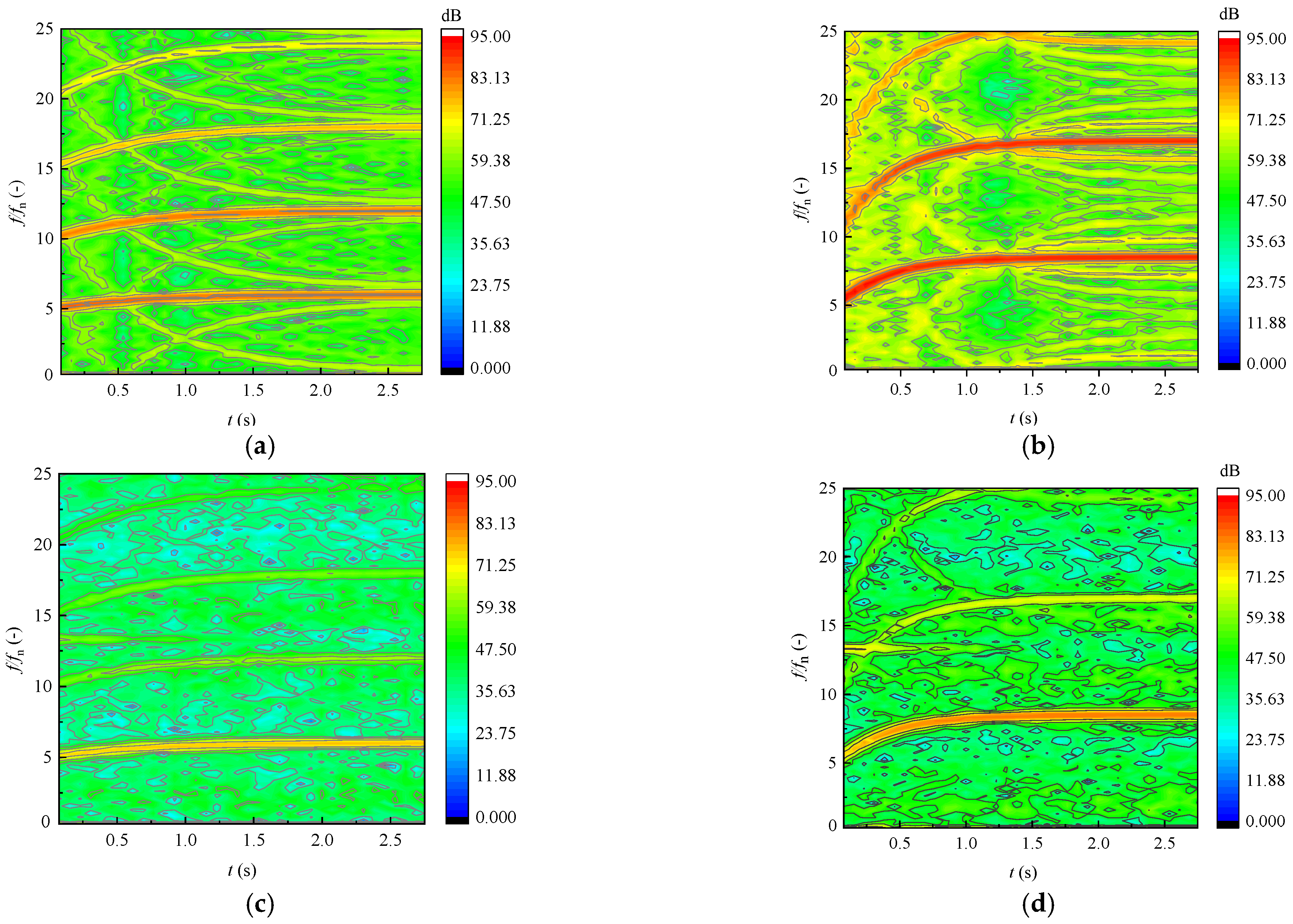
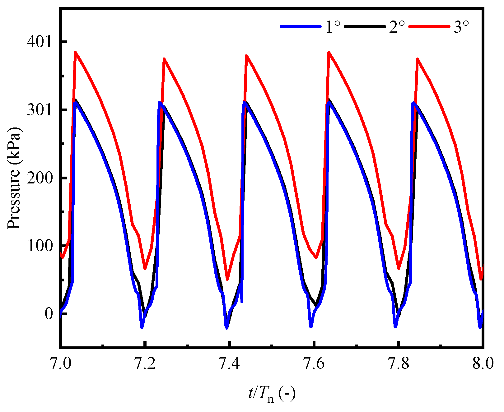
4.2.2. Analysis of the Pressure Pulsation Characteristics

To comprehensively analyze the pressure pulsation characteristics of the tubular turbine during the runaway process, four monitoring points are set up at typical positions in each area of the turbine flow channel, which are arranged at the M1 point in the guide vane area, the M2 point in the runner area, the M3 point in the straight cone of the draft tube, and the M4 point downstream of the straight cone section of the draft tube, as shown in Figure 12.

Figure 13 lists the variation characteristics of pressure with time at four typical monitoring points during the runaway of the turbine when the initial steady state flow rates are 0.85Q_BEP and 1.1Q_BEP. Under the two working conditions, the pressure change trends of the corresponding monitoring points are basically the same. In addition, monitoring point M1 is basically the same as the system return water pressure, and both gradually decrease and become stable with the development of the runaway process. The pressure at the M2 point gradually increases with the development of the runaway process and becomes stable under different initial conditions. Furthermore, the pressure at the M2 point at the start of the runaway has a relatively large pressure oscillation, and the operation of the unit is extremely dangerous under such a large pulsation condition. In the comparison of the two working conditions, the pressure oscillation phenomenon at the M2 point has a larger amplitude under the 1.1Q_BEP working condition, but the duration is relatively short. The duration is about half of that under the 0.85Q_BEP working condition. Point M3 is close to the runner, so its change is basically similar to that of point M2, showing an upward trend with the runaway process. Point M4 is close to the outlet of the draft tube, and its pressure variation law is similar to that of point M1, showing a downward trend with the development of the runaway process.

To determine the time-varying characteristics of the frequency corresponding to the pressure during the runaway of the turbine, the short-time Fourier transform method [19,32] was used in this work to transform the pressure pulsation time domain values of M2 and M3, as shown in Figure 14. The M2 and M3 points show obvious high-amplitude pulsation. The pressure pulsation in the runner domain is related to the rotor–stator interaction. Accordingly, the high amplitude value of the M2 point first appears at the runner blade frequency and its higher harmonics. Furthermore, the main frequency and the magnitude of each harmonic frequency gradually increase with time. These factors remain stable under the runaway state, and the leaf frequency and its higher harmonics always exist in the whole process of runaway development. The comparison of the time–frequency diagrams of points M2 and M3 demonstrates that the change of point M3 is basically the same as that of point M2; only the amplitude is small, indicating that the flow at the inlet of the draft tube is greatly affected by the runner. In the comparison of the stable working conditions, the main frequency range corresponding to M2 and M3 significantly increases during the runaway process. The highest point corresponding to the main frequency gradually moves to the high frequency, and the greater the flow rate, the more obvious the change. This phenomenon occurs because the speed of the runner continues to increase during the development of the runaway, causing its main frequency to gradually increase along the direction of the speed change, and the main frequency also reaches the maximum when the speed reaches the runaway speed.

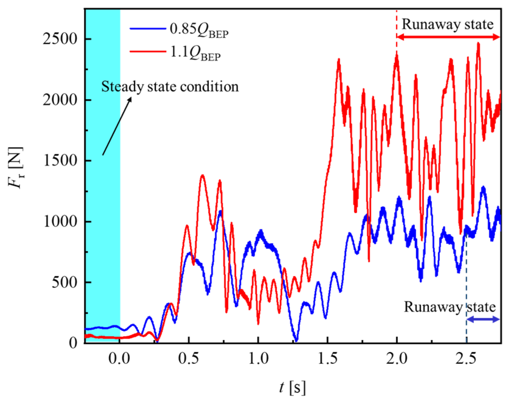
4.2.3. Analysis of the Force Characteristics of the Runner

The uneven flow state in the turbine will cause an uneven force on the runner, generate a large radial force, and affect the stability of the unit. The radial force of the runner during the rotation process can be decomposed into forces in the x and y directions because the main axis of the calculation model is along the Z axis. The radial force and the component forces in the x and y directions are denoted as F_r, F_x, and F_y, respectively, and the calculation Equation is as follows [33]:

$$F_{\mathrm{x}}+{\displaystyle {\iint }_{A_2}\cos ({\theta }^{\prime }+\omega t)p(r_2,\theta )\mathrm{d}A}+\rho \frac{\partial }{\partial t}{\displaystyle {\int }_V\mathrm{d}Q{V}_{\mathrm{x}}}-\left({\displaystyle {\iint }_{A_2}{V}_{\mathrm{x}}\rho V_{\mathrm{r}}\mathrm{d}A-{\displaystyle {\iint }_{A_1}{V}_{\mathrm{x}}\rho V_{\mathrm{r}}\mathrm{d}A}}\right)=0,$$

(20)

$$F_{\mathrm{y}}+{\displaystyle {\iint }_{A_2}\sin ({\theta }^{\prime }+\omega t)p(r_2,\theta )\mathrm{d}A}+\rho \frac{\partial }{\partial t}{\displaystyle {\int }_V\mathrm{d}Q{V}_{\mathrm{y}}}-\left({\displaystyle {\iint }_{A_2}{V}_{\mathrm{y}}\rho V_{\mathrm{r}}\mathrm{d}A-{\displaystyle {\iint }_{A_1}{V}_{\mathrm{y}}\rho V_{\mathrm{r}}\mathrm{d}A}}\right)=0,$$

(21)

$$F_{\mathrm{r}}=\sqrt{F_{\mathrm{x}}^2+F_{\mathrm{y}}^2},$$

(22)

where A₁ represents the cross-sectional area of the runner inlet; V_r is the radial velocity of the fluid particle; V_x and V_y represent the component velocities of the fluid particle in the x and y directions, respectively; ω is the rotational angular velocity of the runner; θ is the initial angle of the fluid particle; t is time; and P is pressure.

Figure 15 shows the time domain diagram of the radial force on the runner during the runaway process under the two operating conditions. In the development process of the runaway, the radial force has a similar increasing trend under the two working conditions. The increasing and decreasing nodes of the radial force in the small flow rate condition lag behind the large flow rate condition. This phenomenon is related to the longer time required for the speed to reach the runaway state under low flow rate conditions. In the initial stage (t < 0.25 s) after the turbine loses its load due to inertia, the radial force is basically close to the initial steady state condition. In addition, the radial force has an obvious local minimum phenomenon in the middle stage of runaway development (about t = 1 and 1.25 s) under the two working conditions. In the middle and late stages of the runaway development, the fluctuation of the radial force with time is similar to the runaway state because the rotational speed is close to the runaway speed at this time, and it shows a violent oscillation phenomenon with time.

Table 4. Comparison of the maximum values of Fr before and after the turbine runaway.

Initial Steady State Condition Turbine Flow Rate	Fr Maximum (N)
	Initial Steady State Condition	Runaway State
0.85QBEP	157	1290
1.1QBEP	68	2510

shows the comparison of the maximum value of Fr before and after the turbine runaway. Under the initial flow rate of 0.85Q_BEP, the maximum radial force on the runner increases from 157 N in the initial steady state to 1290 N, an increase of 1133 N, and the radial force maximum value in the runaway state is 7 times that of the initial steady state. At the initial flow rate of 1.1Q_BEP, the maximum radial force on the runner increased from 68 N in the initial steady state to 2510 N, an increase of 2442 N, and the maximum radial force is 37 times that of the initial steady state during the runaway state.

The time domain diagram of the radial force component of the runner under two flow rate conditions (0.85Q_BEP, 1.1Q_BEP) is drawn to further analyze the variation law of the component forces of the radial force in the x and y directions during the runaway development process, as shown in Figure 16. In the process of runaway development, the component forces of the radial force in the x and y directions substantially increase, and the increase is consistent. In the middle stage of runaway development, the components of radial force in the x and y directions are significantly reduced. In particular, the component forces in both directions are close to zero in the small flow rate condition.

The larger fluctuation of the radial force of the runner can make the rotating shaft of the hydro turbine set eccentric, causing the shaft whirl, aggravating the wear of the shafting, and even resulting in accidents, such as the collision between the rotor and the stator. Therefore, protective shutdown measures must be taken as soon as possible after the turbine runs away.

4.3. Analysis on the Opening and Closing Law of the Control Valve during the Shutdown Process of the Turbine Runaway State

From the previous analysis, the turbine must not run for a long time after a runaway fault. The turbine must be timely cut off from the system, and the system pressure should be restored to the steady state before the runaway. Unlike the large tubular hydropower station, the turbine in this study is of fixed guide vane and paddle structure. Moreover, the shutdown process of the turbine is realized by operating the control valve on the pipeline. Closing the valve or opening the valve in a shorter time can easily lead to positive or negative water hammer in the system [34,35], which seriously threatens the safe operation of the system equipment.

This work compares the variation law of system return water pressure under different opening and closing schemes of valves V₂ and V₁. In each scheme, valves V₂ and V₁ are linearly closed or opened. The operating time of the two valves is used as the optimization variable. The optimization goal is to limit excessive positive and negative water hammer peaks and water hammer durations. The tubular turbine takes less than 3 s to run away from the start to the runaway state, and it generally takes several seconds for the actuator to operate from receiving the command. Therefore, the faulty turbine has been in the runaway state when valves V₁ and V₂ execute the shutdown command. In this paper, the initial time of runaway process is 0 s, and the valve starts to operate from the 3 s. According to the hydraulic characteristics of the valve provided by the manufacturer, the hydraulic opening of valve V₁ is equivalent to the turbine resistance when the hydraulic opening rates are 39% and 34% when the flow rates are 0.85Q_BEP and 1.1Q_BEP, respectively.

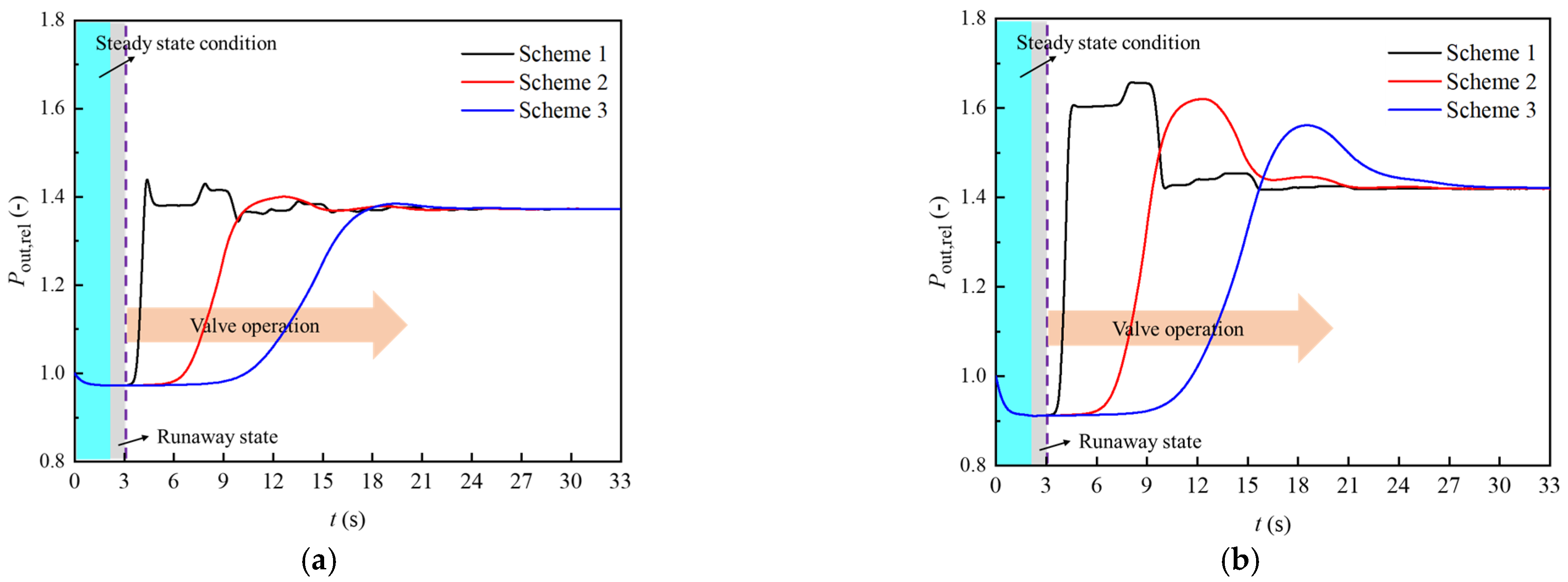
4.3.1. Process Analysis of Separate Closure of Tandem Valves

In this transient process, valve V₁ remains closed, and valve V₂ considers three types of linear closing time. The specific scheme is shown in

Table 5. Close valve schemes.

Scheme	V1 Valve	V2 Valve
Scheme 1	Fully closed state	Linear off, 2 s fully off
Scheme 2	Fully closed state	Linear off, 10 s fully off
Scheme 3	Fully closed state	Linear off, 20 s fully off

.

Figure 17 shows the variation law of P_out,rel under different valve closing schemes of valve V₂. The three valve closing schemes under the working conditions of 0.85Q_BEP and 1.1Q_BEP will generate a larger positive water hammer. The peak pressure of the positive water hammer increases with the shortening of the valve closing time of V₂, but the propagation time of the water hammer wave is short. Under the scheme 1, when the initial steady-state flow rate is 0.85Q_BEP and 1.1Q_BEP, the maximum P_out,rel is 1.43 and 1.67 times of the initial steady-state condition, respectively. When the initial steady state flow rate before runaway is 0.85Q_BEP, valve V₂ is closed alone, and the final system return water pressure is 37% higher than the target pressure. When the initial steady state flow rate before runaway is 1.1Q_BEP, the valve V₂ is closed alone, and the final system return water pressure is 42% higher than the target pressure. Therefore, closing the system pressure of valve V₂ alone will affect the safety of system operation due to excessive positive water hammer.

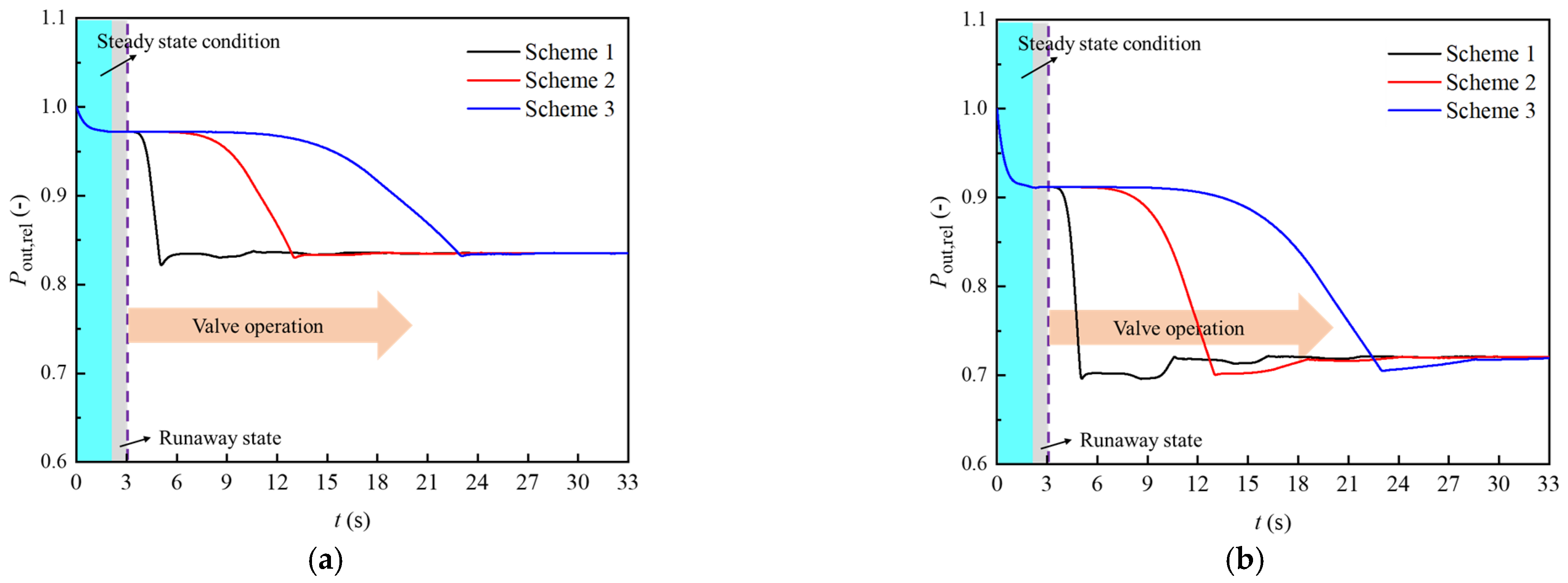
4.3.2. Analysis of the Separate Opening Process of the Parallel Valve

In this transient process, valve V₂ remains fully open, and valve V₁ is linearly opened to 49% of the opening degree considering three durations. The specific scheme is shown in

Table 6. Open valve schemes.

Scheme	V1 Valve	V2 Valve
Scheme 1	Linear opening, 2 s opening to resistance equivalent opening	Fully open
Scheme 2	Linear opening, 10 s opening to resistance equivalent opening	Fully open
Scheme 3	Linear opening, 20 s opening to resistance equivalent opening	Fully open

.

Figure 18 shows the variation law of P_out,rel under different valve opening schemes of valve V₁. The three valve opening schemes under 0.85Q_BEP and 1.1Q_BEP conditions will generate a larger negative water hammer. The valley value of the negative water hammer decreases with the shortening of the valve opening time of V₁. However, the propagation time of the water hammer wave is short. Under the scheme 1, when the initial steady-state flow rate is 0.85Q_BEP and 1.1Q_BEP, the maximum P_out,rel is 0.83 and 0.69 times of the initial steady-state condition, respectively.

When the initial steady state flow rate before runaway is 0.85Q_BEP, the final system return water pressure is 16% lower than the target pressure when valve V₁ is opened alone. When the initial steady state flow rate before runaway is 1.1Q_BEP, the final system return water pressure is 28% lower than the target pressure when valve V₁ is opened alone. When valve V₁ is opened alone, the system pressure will affect the safety of the system operation due to excessive negative water hammer. Accordingly, the system pressure fluctuation increases with the increase in the initial steady-state flow rate before runaway.

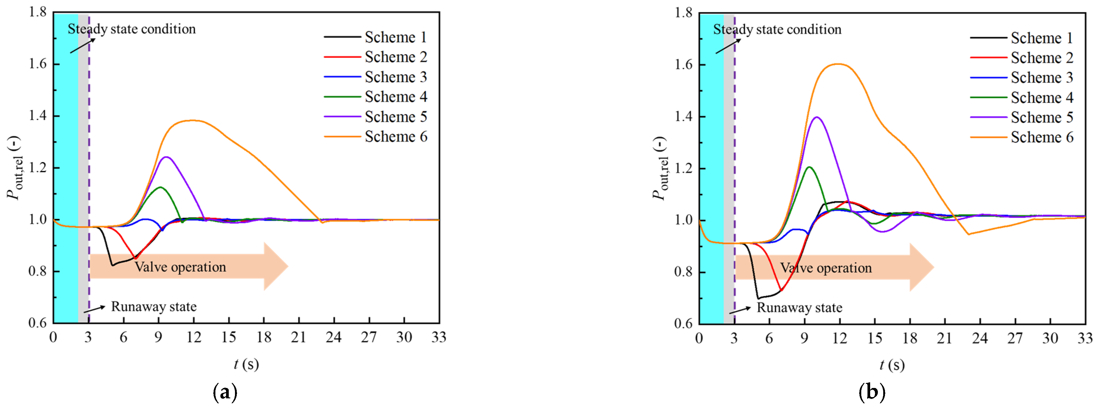
4.3.3. Synergistic Control Analysis of the Series and Parallel Valves

Closing V₂ alone or opening V₁ alone will affect the safety of system operation. Therefore, V₂ and V₁ must be simultaneously operated. The specific scheme is shown in

Table 7. Valve co-operation schemes.

Scheme	V1 Valve	V2 Valve
Scheme 1	Linear opening, 2 s opening to resistance equivalent opening	Linear off, 10 s fully off
Scheme 2	Linear opening, 4 s opening to resistance equivalent opening	Linear off, 10 s fully off
Scheme 3	Linear opening, 6 s opening to resistance equivalent opening	Linear off, 10 s fully off
Scheme 4	Linear opening, 8 s opening to resistance equivalent opening	Linear off, 10 s fully off
Scheme 5	Linear opening, 10 s opening to resistance equivalent opening	Linear off, 10 s fully off
Scheme 6	Linear opening, 20 s opening to resistance equivalent opening	Linear off, 10 s fully off

.

Figure 19 shows the calculation results under the six valve synergy operation schemes. When the operation time of valve V₁ is the same as the valve closing time of V₂, the positive pressure wave in the return water pressure will be large. When the operating time of valve V₁ is longer than the closing time of V₂, the peak value of the positive pressure wave will increase. Meanwhile, when the operation time of valve V₁ is less than the valve closing time of V₂, the peak value of the positive pressure wave gradually decreases as the operation time of valve V₁ shortens. However, an excessively short valve opening time will produce a smaller negative pressure valley. When the initial steady state flow rate before runaway is 0.85Q_BEP, the final system return water pressure is 18% lower than the initial steady-state condition when adopt scheme 1, and the final system return water pressure is 38% higher than the initial steady-state condition when adopt scheme 6. When the initial steady state flow rate before runaway is 1.1Q_BEP, the final system return water pressure is 31% lower than the initial steady-state condition when adopt scheme 1, and the final system return water pressure is 60% higher than the initial steady-state condition when adopt scheme 6. The comparison of the calculation results of the six schemes under the two initial flow rates before runaway shows that the operating time of valve V₁ should be less than the closing time of V₂, and the reasonable coordinated operation of V₁ and V₂ can effectively suppress the fluctuation of return water pressure. When the valve opening time of V₁ is 60% of the valve closing time of V₂ (scheme 3), the system studied in this work is relatively optimal under large and small flow rate conditions.

In addition, valve V₁ must meet the automatic grid-connected operation conditions under different working conditions because the operating conditions of the hydraulic turbine vary. Accordingly, the setting value of the equivalent flow resistance opening of valve V₁ and the hydraulic turbine should be based on the hydraulic turbine under the steady state operating conditions. The running traffic is updated in real time.

5. Conclusions

In this study, a 1D MOC–3D CFD coupled simulation method was developed for CCWS with tubular turbines to successfully simulate the runaway and runaway shutdown process of tubular turbines under small and large flow rate conditions in the real system for studying the influence of runaway of tubular turbines on the stability of CCWS.

(1)

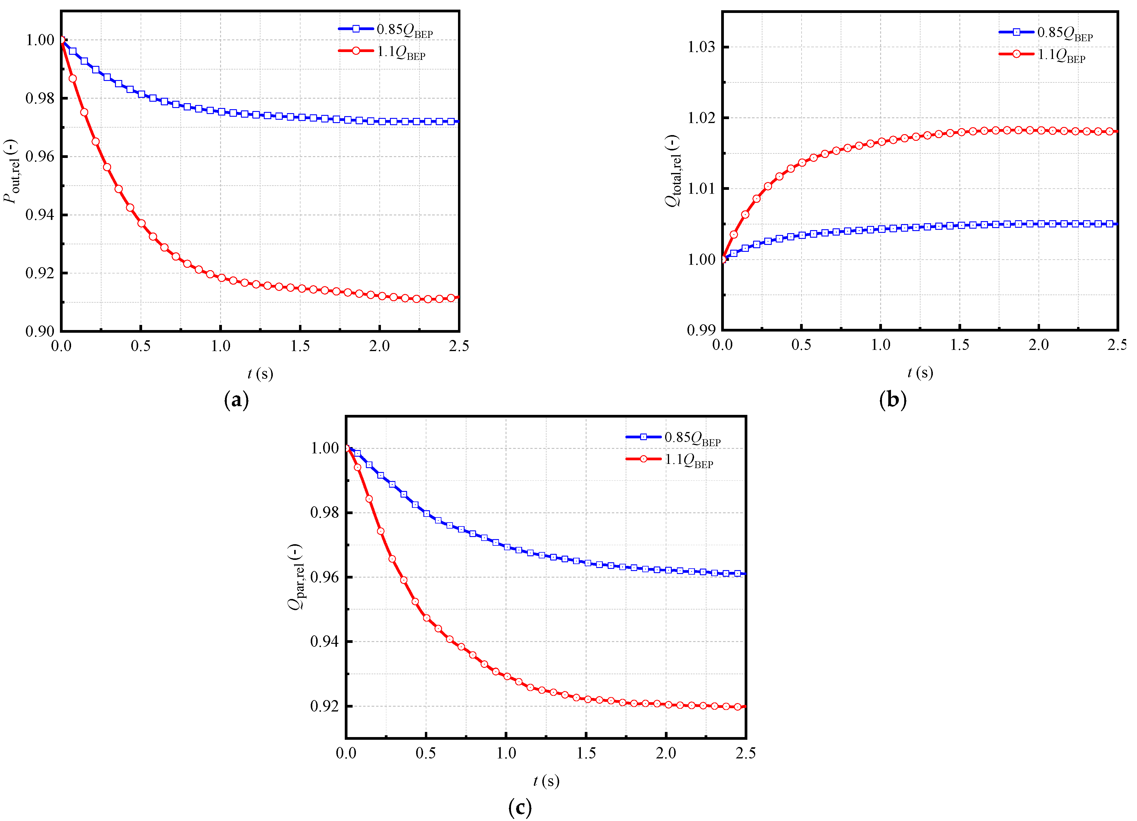
After the tubular turbine entered the runaway process, it did not cause major water hammer problems to the system. Before and after the runaway of the fault turbine, when the initial steady-state flow rate of the turbine is 0.85Q_BEP and 1.1Q_BEP, the return water pressure of the system decreases by 3% and 9%, the system flow rate increases by 0.5% and 1.8%, and the flow rate of the turbine in parallel with the fault turbine decreases by 4% and 8% respectively.

(2)

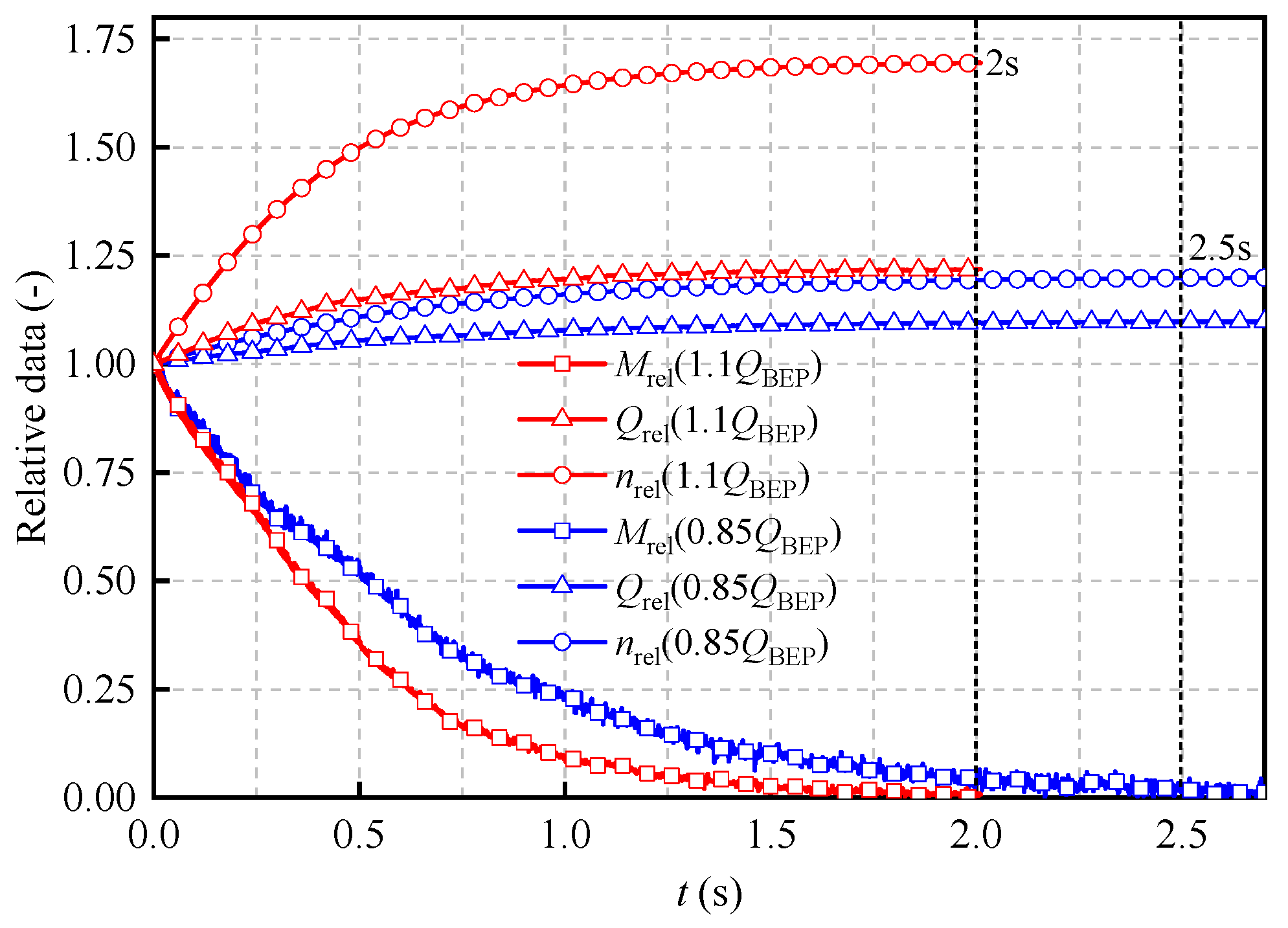
When the tubular turbine enters the runaway process from the steady-state condition, the fault turbine shows the characteristics of increasing speed and flow rate. The change rates of speed and flow rate are great, and the time from the initial state to the runaway state is short with the increase in the initial flow rate. When the initial flow rate is 0.8QBEP, the runaway speed and flow rate of the turbine are 1.2 and 1.1 times the initial steady-state condition, respectively. When the initial flow rate is 1.1QBEP, the runaway speed and flow rate of the turbine are 1.7 and 1.2 times the initial steady-state condition, respectively. At the beginning of the runaway process, the pressure at the monitoring points in the runner area greatly fluctuated. The pressure oscillation amplitude of the monitoring points in the runner area increases with the increase in the initial steady-state flow rate, but the duration decreases. In addition, the radial force of the fault turbine runner in the runaway state greatly increases and shows violent oscillation compared with the initial steady-state condition. When the initial steady-state flow rate is 0.85QBEP and 1.1QBEP, the maximum radial force is 7 and 37 times the initial steady-state conditions, which will aggravate the shafting wear. Therefore, the runaway of hydraulic turbine in CCWS may lead to serious safety accidents, and it is necessary to shut it down as soon as possible.

(3)

During the shutdown of tubular turbine from runaway state, improper valve control scheme will cause severe positive and negative water hammer in the pipe network and seriously threaten the stable operation of the system. For the research system: Under different flow rate conditions, when the opening time of the parallel valve of the fault turbine is too short compared with the closing time of the series valve, the system return water pressure will produce a negative pressure wave, and the valley value of the negative pressure wave is about 69%~82% of the target pressure; On the contrary, when the opening time of the parallel valve is too long compared with the the closing time of the series valve, the return water pressure of the system will produce a positive pressure wave, and the peak value of the positive pressure wave is about 138%~160% of the target pressure; When the opening time of the parallel valve is 60% of the closing time of the series valve, the operating pressure of the system will return to the initial steady state smoothly.

References

1. Zhu, X.; Niu, D.; Wang, X.; Wang, F.; Jia, M. Comprehensive energy saving evaluation of circulating cooling water system based on combination weighting method. Appl. Therm. Eng. 2019, 157, 113735. [Google Scholar] [CrossRef]
2. Wang, P.; Lu, J.; Cai, Q.; Chen, S.; Luo, X. Analysis and Optimization of Cooling Water System Operating Cost under Changes in Ambient Temperature and Working Medium Flow. Energies 2021, 14, 6903. [Google Scholar] [CrossRef]
3. Gao, W.; Feng, X. The power target of a fluid machinery network in a circulating water system. Appl. Energy 2017, 205, 847–854. [Google Scholar] [CrossRef]
4. Ma, J.; Wang, Y.; Feng, X. Energy recovery in cooling water system by hydro turbines. Energy 2017, 139, 329–340. [Google Scholar] [CrossRef]
5. Li, Y.; Yuan, S.; Che, D. Utilization of residual energy of industrial circulating cooling water and its key technologies. J. Drain. Irrig. Mech. Eng. 2015, 7, 667–673. (In Chinese) [Google Scholar]
6. Chen, H.; Zhou, D.; Kan, K.; Xu, H.; Zheng, Y.; Binama, M.; Xu, Z.; Feng, J. Experimental investigation of a model bulb turbine under steady state and load rejection process. Renew. Energy 2021, 169, 254–265. [Google Scholar] [CrossRef]
7. Aponte, R.D.; Teran, L.A.; Grande, J.F.; Coronado, J.J.; Ladino, J.A.; Larrahondo, F.J.; Rodríguez, S.A. Minimizing erosive wear through a CFD multi-objective optimization methodology for different operating points of a Francis turbine. Renew. Energy 2020, 145, 2217–2232. [Google Scholar] [CrossRef]
8. Whitacker, L.H.L.; Tomita, J.T.; Bringhenti, C. Effect of tip clearance on cavitating flow of a hydraulic axial turbine applied in turbopump. Int. J. Mech. Sci. 2022, 213, 106855. [Google Scholar] [CrossRef]
9. Zhang, H.; Chen, D.; Wu, C.; Wang, X.; Lee, J.-M.; Jung, K.-H. Dynamic modeling and dynamical analysis of pump-turbines in S-shaped regions during runaway operation. Energy Convers. Manag. 2017, 138, 375–382. [Google Scholar] [CrossRef] [Green Version]
10. Zhan, J. Analysis and treatment of runaway fault of unit in Feilaixia Hydropower Plant. Guide Get. Rich Sci. Technol. 2010, 2, 165–318. (In Chinese) [Google Scholar]
11. Li, H.; Guo, L. Accident treatment of broken pin of bulb tubular turbine. Eng. Technol. 2015, 43, 116. (In Chinese) [Google Scholar]
12. Feng, J.; Li, W.; Luo, X.; Zhu, G. Numerical analysis of transient characteristics of a bulb hydraulic turbine during runaway transient process. Proc. Inst. Mech. Eng. Part E J. Process Mech. Eng. 2018, 233, 813–823. [Google Scholar] [CrossRef]
13. Chen, M.; Guo, J.; Sun, J. Influence of blade opening on runaway process of tubular turbine. Hydropower Energy Sci. 2022, 40, 4. (In Chinese) [Google Scholar]
14. Ghidaoui, M.S.; Zhao, M.; McInnis, D.A.; Axworthy, D.H. A Review of Water Hammer Theory and Practice. Appl. Mech. Rev. 2005, 58, 49–76. [Google Scholar] [CrossRef]
15. Lister, M. The numerical solution of hyperbolic partial differential equations by the method of characteristics. Math. Methods Digit. Comput. 1960, 1, 165–179. [Google Scholar]
16. Singhal, A.K.; Athavale, M.M.; Li, H.; Jiang, Y. Mathematical Basis and Validation of the Full Cavitation Model. J. Fluids Eng. 2002, 124, 617–624. [Google Scholar] [CrossRef]
17. Wang, W.; Pavesi, G.; Pei, J.; Yuan, S. Transient simulation on closure of wicket gates in a high-head Francis-type reversible turbine operating in pump mode. Renew. Energy 2020, 145, 1817–1830. [Google Scholar] [CrossRef]
18. Li, Y.; Song, G.; Yan, Y. Transient hydrodynamic analysis of the transition process of bulb hydraulic turbine. Adv. Eng. Softw. 2015, 90, 152–158. [Google Scholar] [CrossRef]
19. Yang, S.; Chen, X.; Wu, D.; Yan, P. Dynamic analysis of the pump system based on MOC–CFD coupled method. Ann. Nucl. Energy 2015, 78, 60–69. [Google Scholar] [CrossRef]
20. Li, Z.; Bi, H.; Karney, B.; Wang, Z.; Yao, Z. Three-dimensional transient simulation of a prototype pump-turbine during normal turbine shutdown. J. Hydraul. Res. 2017, 55, 520–537. [Google Scholar] [CrossRef]
21. Liu, D.; Zhang, X.; Yang, Z.; Liu, K.; Cheng, Y. Evaluating the pressure fluctuations during load rejection of two pump-turbines in a prototype pumped-storage system by using 1D-3D coupled simulation. Renew. Energy 2021, 171, 1276–1289. [Google Scholar] [CrossRef]
22. Yang, Z.; Cheng, Y.; Xia, L.; Meng, W.; Liu, K.; Zhang, X. Evolutions of flow patterns and pressure fluctuations in a prototype pump-turbine during the runaway transient process after pump-trip. Renew. Energy 2020, 152, 1149–1159. [Google Scholar] [CrossRef]
23. Fu, X.; Li, D.; Wang, H.; Li, Z.; Zhao, Q.; Wei, X. One- and three-dimensional coupling flow simulations of pumped-storage power stations with complex long-distance water conveyance pipeline system. J. Clean. Prod. 2021, 315, 128228. [Google Scholar] [CrossRef]
24. Zhang, W. Partial Differential Equation Finite Difference Method in Scientific Calculation; Higher Education Press: Beijing, China, 2006. (In Chinese) [Google Scholar]
25. Wang, L.; Xu, X. The Mathematical Basis of Finite Element Method; Science Press: Beijing, China, 2004. (In Chinese) [Google Scholar]
26. Tan, W. Computational Shallow Water Dynamics: Application of Finite Volume Method; Tsinghua University Press: Beijing, China, 1998. (In Chinese) [Google Scholar]
27. Ye, W.; Geng, C.; Luo, X. Unstable flow characteristics in vaneless region with emphasis on the rotor-stator interaction for a pump turbine at pump mode using large runner blade lean. Renew. Energy 2022, 185, 1343–1361. [Google Scholar] [CrossRef]
28. Zhang, X.; Cheng, Y.; Yang, Z.; Chen, Q.; Liu, D. Water column separation in pump-turbine after load rejection: 1D-3D coupled simulation of a model pumped-storage system. Renew. Energy 2020, 163, 685–697. [Google Scholar] [CrossRef]
29. Zhang, X.X.; Cheng, Y.G. Simulation of hydraulic transients in hydropower systems using the 1-D-3-D coupling approach. J. Hydrodyn. Ser. B 2012, 24, 595–604. [Google Scholar] [CrossRef]
30. Walski, T.M.; Daviau, J.L.; Coran, S. Effect of Skeletonization on Transient Analysis Results. In Proceedings of the World Water & Environmental Resources Congress, Salt Lake City, UT, USA, 27 June–1 July 2004. [Google Scholar]
31. Castro, M.M.; Song, T.W.; Pinto, J.M. Minimization of Operational Costs in Cooling Water Systems. Chem. Eng. Res. Des. 2000, 78, 192–201. [Google Scholar] [CrossRef]
32. Su, W.-T.; Li, X.-B.; Xia, Y.-X.; Liu, Q.-Z.; Binama, M.; Zhang, Y.-N. Pressure fluctuation characteristics of a model pump-turbine during runaway transient. Renew. Energy 2020, 163, 517–529. [Google Scholar] [CrossRef]
33. Zhang, M.; Wang, H.; Tsukamoto, H. Numerical Analysis of Unsteady Hydrodynamic Forces on a Diffuser Pump Impeller Due to Rotor-Stator Interaction. In Proceedings of the ASME 2002 Joint U.S.-European Fluids Engineering Division Conference. Volume 2: Symposia and General Papers, Parts A and B, Montreal, QC, Canada, 14–18 July 2002; pp. 751–760. [Google Scholar]
34. Wei, Z.; Yin, G.; Wang, J.; Wan, L.; Jin, L. Stability analysis and supporting system design of a high-steep cut soil slope on an ancient landslide during highway construction of Tehran–Chalus. Environ. Earth Sci. 2012, 67, 1651–1662. [Google Scholar] [CrossRef]
35. Yang, Z.; Zhou, L.; Dou, H.; Lu, C.; Luan, X. Water hammer analysis when switching of parallel pumps based on contra-motion check valve. Ann. Nucl. Energy 2019, 139, 107275. [Google Scholar] [CrossRef]
Figure 1. Recovery of the CCWS surplus back pressure energy with a tubular turbine.
Water 14 02294 g001
Figure 2. Positive and negative water hammer characteristic lines.
Water 14 02294 g002
Figure 3. Simplified schematic of the boundary conditions during a normal operation of the pumping station.
Water 14 02294 g003
Figure 4. Interface of the coupling algorithm with overlapping meshes.
Water 14 02294 g004
Figure 5. Coupling interface data transfer mechanism. (a) Turbine inlet coupling interface. (b) Turbine outlet coupling interface.
Water 14 02294 g005
Figure 6. Time step independence verification.
Water 14 02294 g006
Figure 7. Comparison of the experimental and numerical simulation results.
Water 14 02294 g007
Figure 8. Schematic of the Coupled model.
Water 14 02294 g008
Figure 9. Comparison of the 1D MOC and coupled algorithm results.
Water 14 02294 g009
Figure 10. Influence of the turbine runaway on the system return water pressure, system flow rate, and parallel turbine flow rate. (a) System return water pressure. (b) System flow rate. (c) Parallel turbine flow rate.
Water 14 02294 g010
Figure 11. Comparison of the working parameters in the runaway process of the turbine.
Water 14 02294 g011
Figure 12. Schematic of the monitoring point layout.
Water 14 02294 g012
Figure 13. Change law of the pressure pulsation at the monitoring point. (a) 0.85QBEP. (b) 1.1QBEP.
Water 14 02294 g013
Figure 14. Time–frequency analysis of the pressure signals at points M2 and M3. (a) 0.85QBEP—M2. (b) 1.1QBEP—M2. (c) 0.85QBEP—M3. (d) 1.1QBEP—M3.
Water 14 02294 g014
Figure 15. Time domain diagram of radial force during runaway.
Water 14 02294 g015
Figure 16. Time domain diagram of the radial force components in the x and y directions during runaway. (a) 0.85QBEP. (b) 1.1QBEP.
Water 14 02294 g016
Figure 17. Variation law of return water pressure under different valve closing schemes. (a) 0.85QBEP. (b) 1.1QBEP.
Water 14 02294 g017
Figure 18. Variation law of the return water pressure under different valve opening schemes. (a) 0.85QBEP. (b) 1.1QBEP.
Water 14 02294 g018
Figure 19. Variation law of the return water pressure under different valve cooperative operation schemes. (a) 0.85QBEP. (b) 1.1QBEP.
Water 14 02294 g019