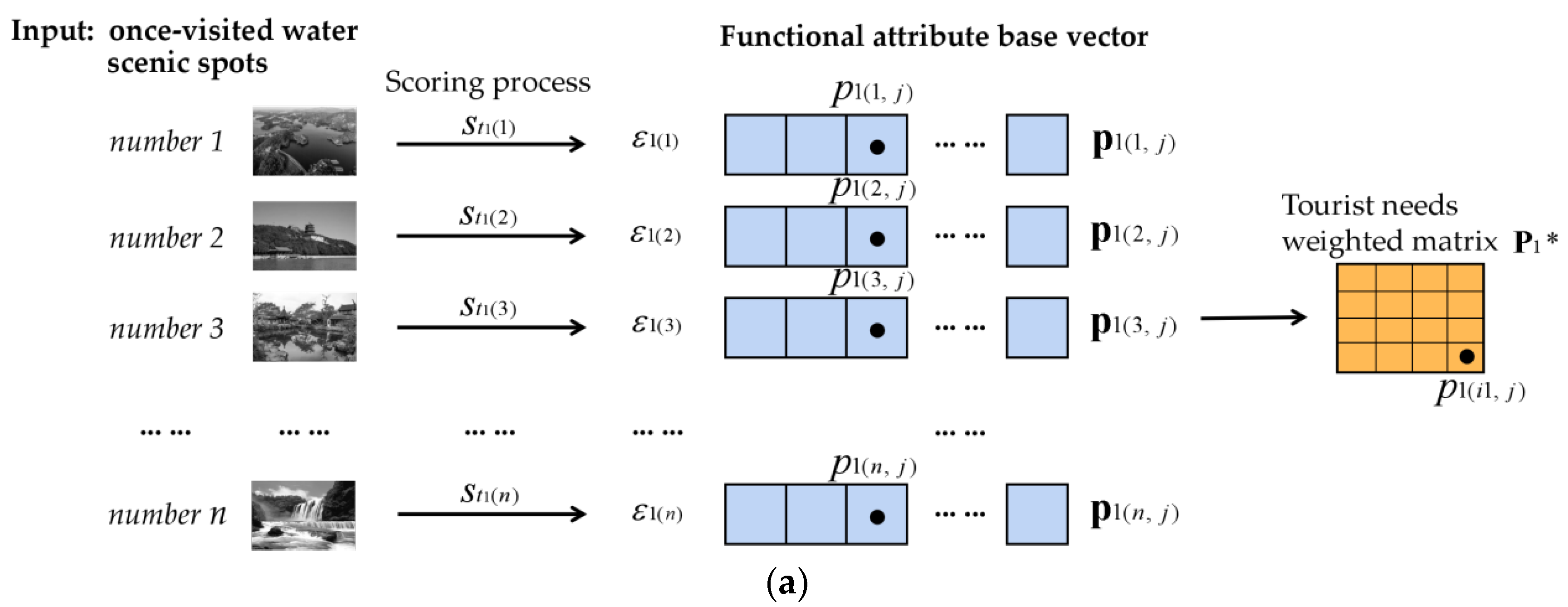
The experiment used the tourism city of Chengdu as the research object, and selected 20 representative water scenic spots in the downtown area of the city. The scenic spots have different functional attributes and can meet the interest needs of different tourists. The experimental principle is as follows: A tourist chooses his favorite once-visited scenic spots, and scores these scenic spots using the percentage system. Then, the evaluation parameters are confirmed. Based on the scenic spot functional attributes, the tourist-demands matrix and the tourist-demands weighted matrix are outputted. By calculating the tourist-needs relative weights, the needs relative weight matrix is obtained. Then, the recommended scenic spot vector is outputted. Based on the vector, the tourist chooses the traffic modes, then the system outputs the water ecotourism route with minimum exhaust emissions through the tour route algorithm. The experiment compares the proposed method with the commonly used route planning methods on maps, and verifies that the proposed method has obvious advantages.
4.4. Experiment Results Analysis and Findings
Of the three aspects of data sampling and processing, the calculation data and results of the water scenic spot recommendation, water tour route recommendation results and comparison results, and the experimental results were analyzed and related conclusions were obtained.
(1) The analysis and findings of the data sampling and processing.
The sampled water scenic spots were analyzed. The water scenic spots are all representative ones in the Chengdu downtown area, and each scenic spot has all-around functional attributes. They were related to the functional attribute base vectors.
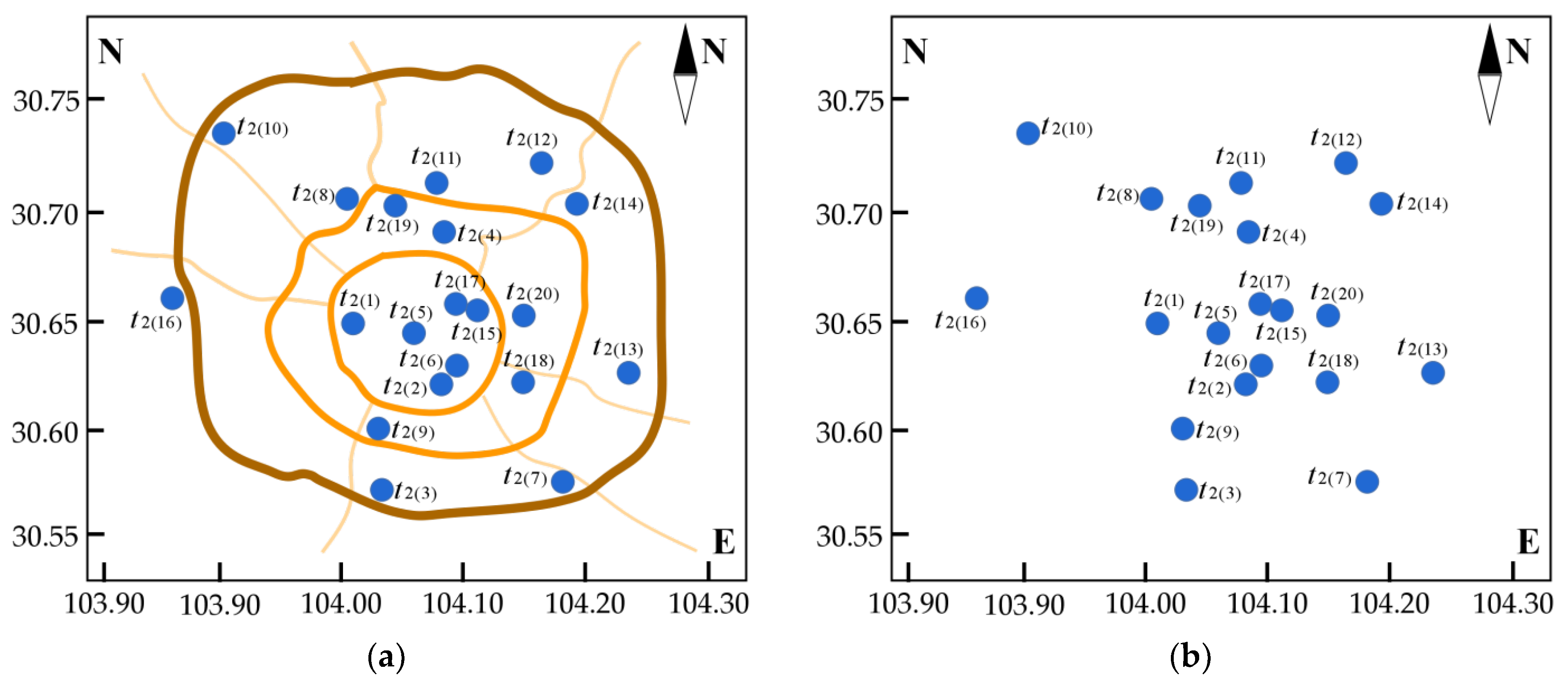
① Finding one: the sampled water scenic spots had strong accessibility.
As seen from
Figure 3, the water scenic spots were uniformly distributed, which meets the requirements of tourists on selecting scenic spots. There were no scenic spots that were too far away from the city center and difficult for tourists to travel to. Therefore, the accessibility of the sampled water scenic spots is strong.
② Finding two: the inputted once-visited water scenic spots reflected the tourist’s interest tendencies.
Analyzing the data in
Table 1, tourists had different preferences in regard to the once-visited scenic spots. They had the greatest preference for
: the Summer Palace, followed by
: Suzhou gardens and
: Guilin landscapes; the lowest preference was for
: Nanjing Xuanwu Lake. It shows that the collected once-visited scenic spots, regarded as the original data for constructing the recommendation algorithm in this paper, can reflect the different interest tendencies of tourists and ensure that the recommendation algorithm can output the matched scenic spots.
③ Finding three: the functional attribute-weighted value influenced the attribute’s capacity for regulating the recommendation result.
Analyzing the data in
Table 2, it can be seen that based on the evaluation parameters of the once-visited water scenic spots and the scenic spot functional attribute base vector, the tourist-needs weighted matrix was outputted, and the matrix element values were the weighted evaluation parameters of the once-visited water scenic spot functional attributes. The functional attribute values of different scenic spots vary with the changes of the water scenic spot evaluation parameters, indicating that the weighted functional attributes of a scenic spot have different intensity effects on the recommendation results. The larger the weighted value is, the greater the effect will be on the recommendation results of the functional attributes related to the weighted value, and vice versa.
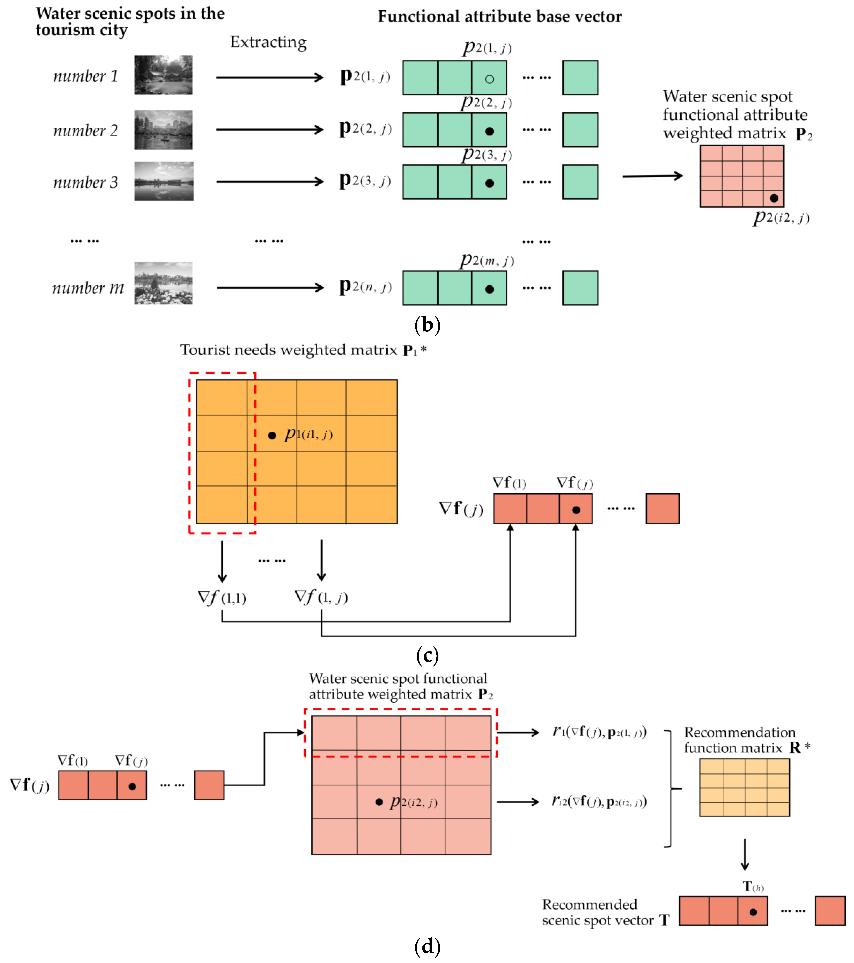
④ Finding four: the sampled water scenic spots have different capacities for satisfying the same tourist’s interests.
Analyzing the data in
Table 3, the sample water scenic spots had different functional attribute vectors and element values, indicating that the capacities of the scenic spots to meet the needs of the same tourist are quite different, and the samples selected in the experiment were diverse. For a scenic spot, the larger the quantity of the element 1 is, the more comprehensive the scenic spot’s functional attributes will be, and more probable that it can meet the tourists’ needs.
(2) The analysis and findings of the calculation data and results of the water scenic spot recommendation.
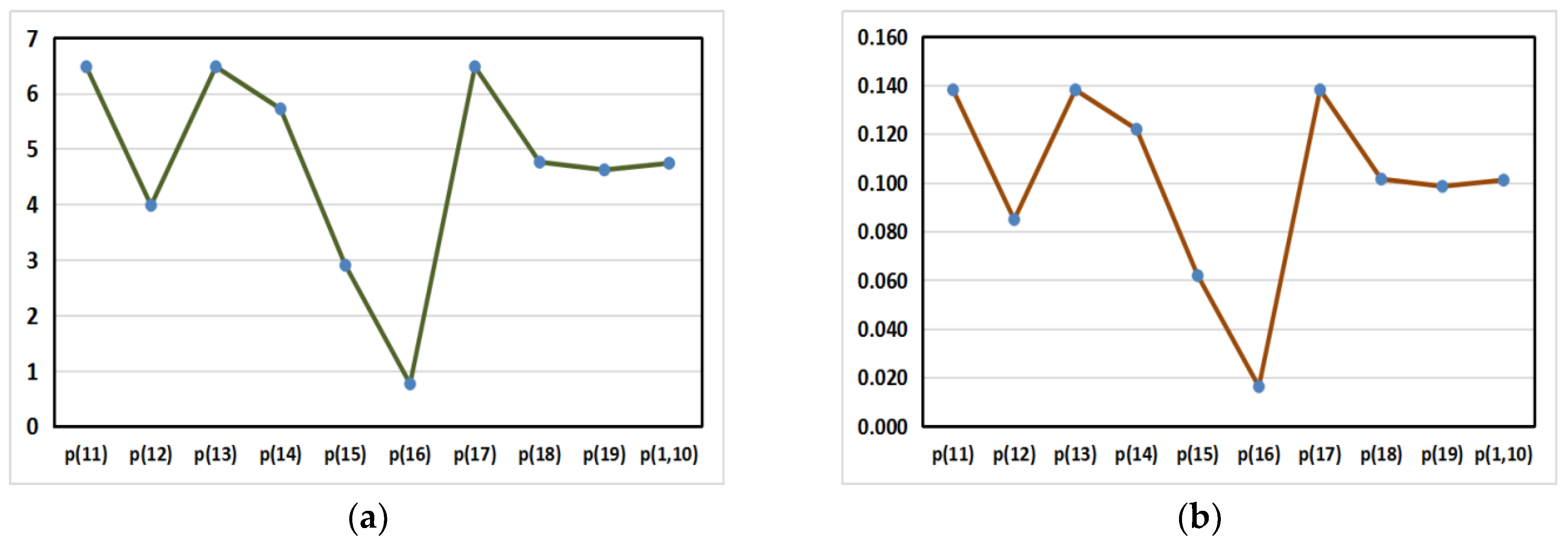
① Finding one: the tourist-needs absolute weights and relative weights directly influenced the recommending results of the functional attributes.
Analyzing the data in
Table 4 and the comparison chart in
Figure 4, it can be seen that the tourist-needs absolute weights and relative weights are different for the once-visited scenic spots. The three functional attributes of
: viewing the water natural scenery,
: water sports, and
: water scenery photography had the highest weight value, which can be interpreted as the three interests meeting the largest proportion of the tourist’s needs, and meaning the tourist is more likely to visit the scenic spots that have the three functional attributes. The functional attribute of
: watching water birds had the lowest weight value, which can be interpreted to mean that the tourist has the lowest need for this attribute. When recommending scenic spots, the absolute weights and relative weights both have important influence, and they directly impact the recommendation results.
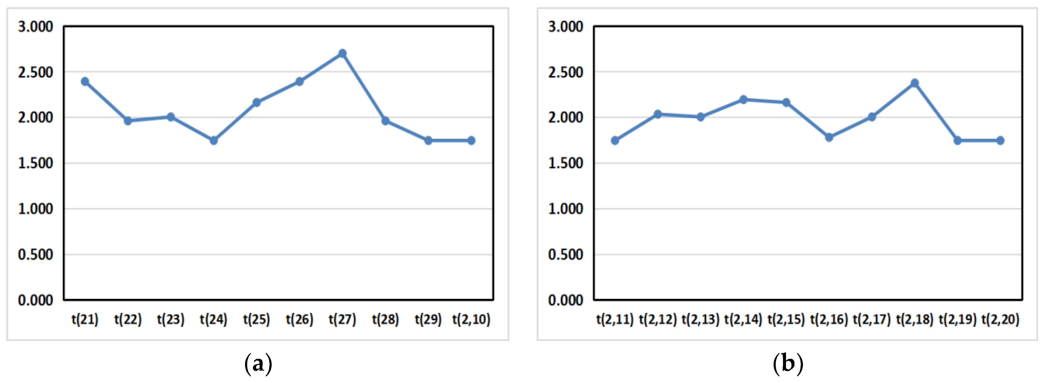
② Finding two: the recommendation function values had direct influence on the recommending results of the water scenic spots.
Analyzing the data in
Table 5 and the comparison chart in
Figure 5, it can be seen that the recommendation function values
outputted by the tourist-needs weight and water scenic spots were greatly different. From the water scenic spot
to
, the function values fluctuated with the scenic spot sequence, in which the scenic spots
,
,
,
,
, and
had the smallest function value; that is, these scenic spots were close to the tourist’s needs. The recommendation system preferentially provided the scenic spots for the tourist.
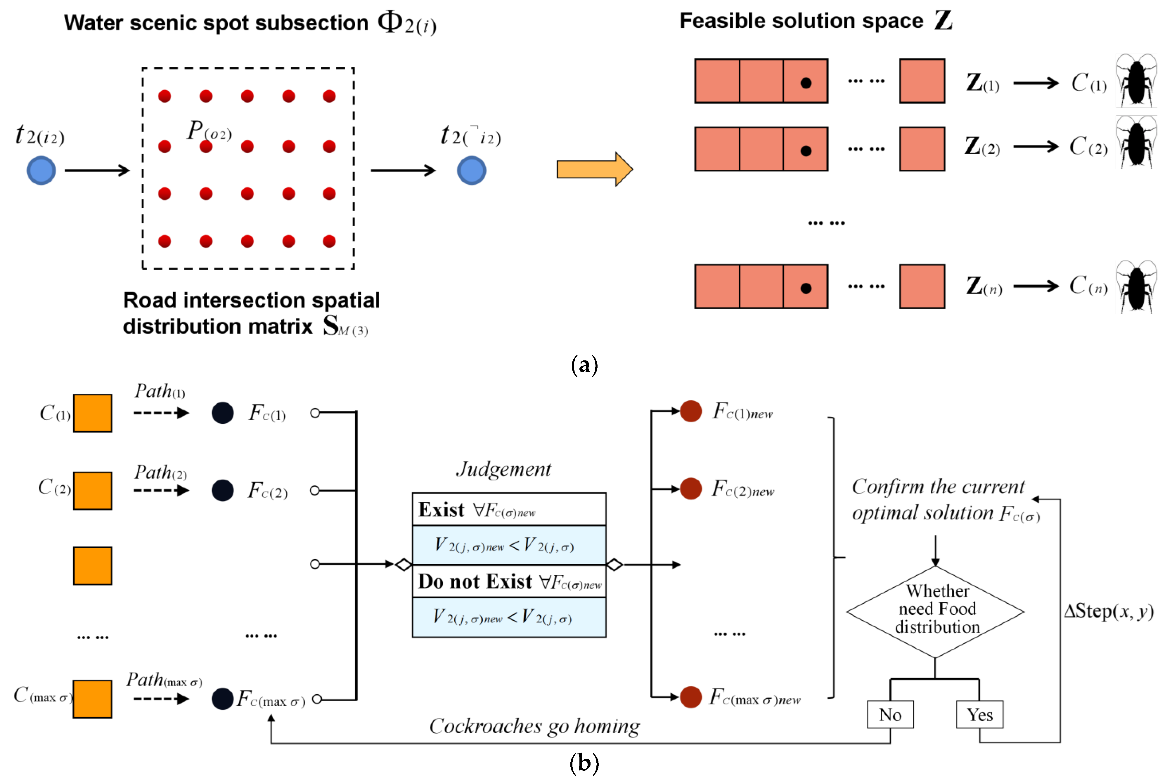
(3) The analysis and findings of the water tour route recommendation and comparison results.
① Finding one: the choice of transportation mode directly influenced the exhaust emission volume, and the three algorithms produced different exhaust emission volumes.
Analyzing the data in
Table 6 and the comparison chart in
Figure 6, it can be seen that there were great differences in the transportation modes among scenic spots selected by tourists according to the recommended results. For those distant scenic spots, tourists tend to take taxis, for scenic spots with moderate distance, tourists tend to take buses, and for those nearby scenic spots, tourists tend to use shared motorcycles. Three optimal tour routes with the lowest exhaust emissions were outputted. The route with the lowest exhaust emissions was
, followed by
and
.
As for the same tour route, the exhaust emissions of the three algorithms varied in different subsections. They fluctuated up and down with the order of the scenic spots’ sequence and the process of sightseeing, and were directly affected by the transportation modes. In the same subsection, the exhaust emissions outputted by the three algorithms were quite different, resulting in great differences of total gas emissions for the whole tour route. According to the transportation modes selected by tourists, when choosing the shared bicycle the exhaust emissions of the tour route is 0, which is the most environmentally friendly way of traveling, but the time cost is the highest.
② Finding two: As to the three recommended tour routes, the PRA produced the lowest exhaust emissions for each subsection and for the whole tour route. Thus, the PRA is superior to the control group algorithms BDA and 360A in the aspect of producing exhaust gases.
(I) Tour route 1:
The subsections with the largest and smallest waste gas generated by PRA were and , respectively. The subsections with the largest and smallest waste gas generated by 360A were and , respectively, and the subsections with the largest and smallest waste gas generated by BDA were and , respectively. In the same subsection, PRA produced the smallest amount of exhaust gas, with both 360A and BDA producing more exhaust gas than PRA. BDA produced the largest amount of exhaust gas in the subsections and , and 360A produced the largest amount of exhaust gas in the subsection . For the whole tour route, PRA produced the smallest amount of waste gas, whereas BDA produced the largest amount of waste gas.
(II) Tour route 2:
The subsections with the largest and smallest waste gas generated by PRA were and , respectively. The subsections with the largest and smallest waste gas generated by 360A were and , respectively, and the subsections with the largest and smallest waste gas generated by BDA were and , respectively. In the same subsection, PRA produced the smallest amount of exhaust gas, with both 360A and BDA producing more exhaust gas than PRA. BDA produced the largest amount of exhaust gas in the subsection , and 360A produced the largest amount of exhaust gas in the subsections and . For the whole tour route, PRA produced the smallest amount of waste gas, whereas 360A produced the largest amount of waste gas.
(III) Tour route 3:
The subsections with the largest and smallest waste gas generated by PRA were and , respectively. The subsections with the largest and smallest waste gas generated by 360A were and , respectively, and the subsections with the largest and smallest waste gas generated by BDA were and , respectively. In the same subsection, PRA produced the smallest amount of exhaust gas, with both 360A and BDA producing more exhaust gas than PRA. BDA produced the largest amount of exhaust gas in the subsections and , and 360A produced the largest amount of exhaust gas in the subsection . For the whole tour route, PRA produced the smallest amount of waste gas, whereas 360A produced the largest amount of waste gas.
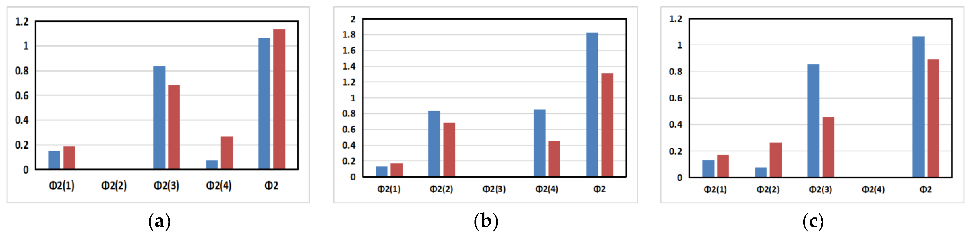
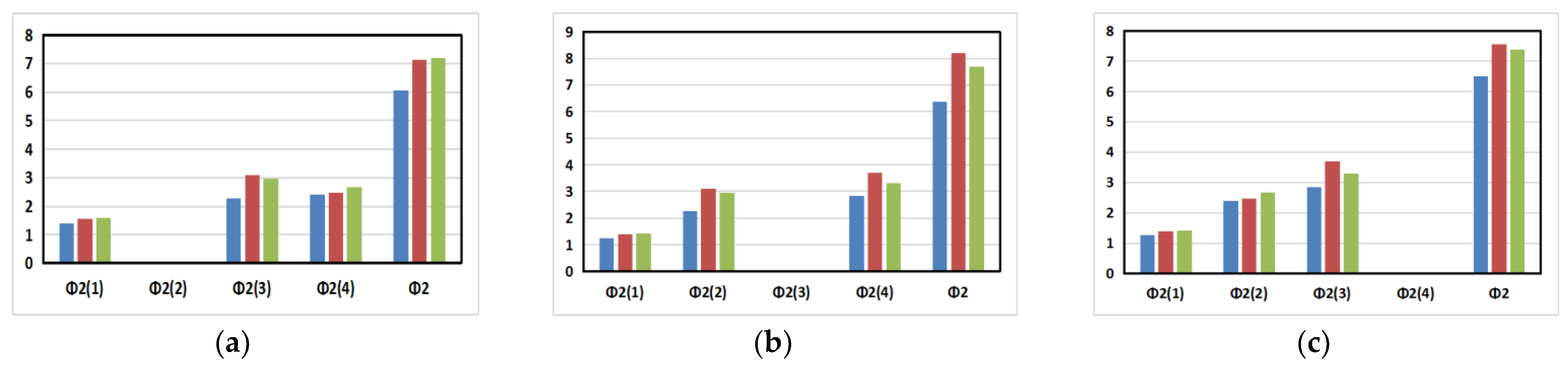
③ Finding three: the control group algorithms BDA and 360A produced more exhaust gases than PRA, and the different volume values between the control group algorithms and PRA were different in each subsection, reaching the maximum for the whole tour route.
Analyzing the comparison diagram in
Figure 7, it can be seen that the exhaust emission volumes of 360A and BDA in each subsection of the three tour routes were larger than PRA, and the difference values between PRA and 360A and between PRA and BDA fluctuated with the subsection’s sequence. In each scenic spot subsection, for the first tour route, the maximum difference value between PRA and 360A appeared at
, and the maximum difference value between PRA and BDA appeared at
. For the second tour route, the maximum difference value between PRA and 360A appeared at
, and the maximum difference value between PRA and BDA appeared at
. For the third tour route, the maximum difference value between PRA and 360A appeared at
, and the maximum difference value between PRA and BDA appeared at
. Each algorithm had the maximum difference value between PRA and 360A and between PRA and BDA for the total tour route.
In conclusion, 360A and BDA are inferior to PRA in the capacity of planning low-carbon tour routes. PRA is relatively more stable. It can find the tour route with the shortest distance and the lowest exhaust emissions, indicating that PRA has better performance and advantages than 360A and BDA in outputting low-carbon tour routes. In each algorithm, the transportation mode had a direct impact on the subsection’s exhaust emissions, the entire tour route exhaust emissions, and the process of outputting the optimal tour route. In this experiment, the tourist chose : public bus as the transportation mode in the subsections and ; thus, the gas emission volume of the tour routes containing the two subsections was very large, and the optimal tour route did not contain the two subsections and . If the tourist chooses : the shared motorcycle as the transportation mode in the subsection , the gas volume produced by a motorcycle will be 0; thus, the optimal tour route must contain the subsection . Since different transportation modes have different unit emissions , PRA integrates the transportation modes selected by tourists in different subsections when searching the tour route. Therefore, the searched tour route is always based on the aim of searching for the lowest exhaust emissions for the entire tour route rather than searching for the shortest distance, which reflects the core idea of the proposed algorithm in the research.
(4) The predicted and long term effects of the proposed algorithm.
Another important finding is the predicted and long-term effects of the proposed algorithm. Since the experiment reflects one sample tourist’s example, it could be interpreted that one tourist’s traveling activities will produce exhaust emissions, and to some extent cause damage to the urban water ecosystem. Based on the fact that there are about 200 million tourists and local residents visiting the water scenic spots in Chengdu every year, if the tour routes and transportation modes recommended in this research are used, the exhaust emissions would be reduced by hundreds of thousands of tons. On the basis of meeting the tourists’ traveling experiences and needs, the proposed method can reduce the damage to the urban water scenic spots and water resources, and protect the urban water ecological environments.


