Real-Time Flood Warning System Application

Abstract

The reliability of weather radar data in real-time flood forecasting and early warning system remain ambivalent due to high uncertainty in Quantitative Precipitation Forecasts (QPF). In this study, a methodology is presented with the objective to improve the flood forecasting results with the application of radar rainfall calculated in three different ways. The QPF radar rainfall forecast data of four typhoon events in Fèngshān River Basin, Taiwan, were simulated using the WASH123D numerical model. The simulated results were corrected using a physical real-time correction technique and compared with direct simulation without correction for all three QPF calculation methods. According to model performance evaluation criteria, in the third method of QPF calculation, flood peak error was the lowest in all three methods, indicating better results for flood forecasting and can be used for flood early warning systems. The impact of the real-time correction technique was assessed using mass balance analysis. It was found that flow change is between 16% and 42% from direct simulation, indicating being on the safe side in case of a flood warning. However, the impact of the real-time physical correction on the water level itself is in a reasonable range. Still, QPF rainfall correction/calculation is more important to obtain accurate results for flood forecasting. Therefore, the application of real-time correction to correct the model water level has a certain degree of credibility, which is the mass balance of the model. This approach is recommended for flood forecasting early warning systems.

1. Introduction

A flood forecasting and warning system deliver reliable and timely information in terms of enough lead-time to civil protection services to take appropriate measures to protect people and their assets from flooding [1]. The effective real-time flood forecasting system is based on a collection of real-time data related to rainfall forecast to flood forecasting model to predict flood severity, time of onset, extent, and magnitude of flooding. Rainfall forecasting is a key meteorological input for flood forecasting, so the reliability of flood forecasting and warning system depends on the accuracy of rainfall forecast and the performance of predictive hydrological models. The use of weather radar rainfall (QPE/QPF: Quantitative Precipitation Estimates and Forecasts) is one of the data collection approaches generally adopted in the design of flood forecasting systems [2]. Literature studies signify the acceptability and reliability of QPE and QPF radar data in hydrological applications, such as Corral et al. [3], Borga et al. [4], and Cole et al. [5]. Chiang and Chang [6], Lin et al. [7], and Yu et al. [8] also supported the capability of radar-based rainfall and encouraged its use in flood forecasting systems. QPF accuracy with respect to lead time is of major concern in the reliability of flood forecasting systems. The lead-time of flood forecasting depends upon the availability of data, hydrometeorological and topographic features of the catchment, and the dynamics of basin response. According to Jian et al. review study, the catchment scale flood forecasting models assembled with updating of QPFs radar rainfall are reliable and comparatively more accurate because of real-time data observed during the lead-time [2].

In Taiwan, three types of flood forecasting systems are used to simulate flood levels such as (1) flood dynamic routing model, (2) rainfall–runoff forecasting model, and (3) rainfall forecasting model. According to Liu and Gupta, there may be three types of uncertainties in flood forecast systems that are caused by various reasons, i.e., (1) parameter uncertainty, (2) model structure uncertainty, and (3) input uncertainty [9]. The input uncertainty in meteorological forecasts precipitation is most important and significantly influences the flood forecasting results than other uncertainties [10,11]. Wu et al. identified that the reliability of a QPF-based flood forecasting system tends to reduce with greater forecasting lead-time due to inherent uncertainties in the system and the mountainous nature of the terrain [12]. The associated input, model structure, and parameter uncertainties in flood forecasting models must be addressed for reliable operations of the early warning system. Therefore, improving the accuracy of the short-term rainfall forecasting model and rainfall–runoff forecasting model is considered essential and continuously focused in Taiwan [13]. However, the accurate prediction of flood peak time and flood peak level according to flood lead-time is fundamentally complex due to the dynamic nature of rainfall and watershed characteristics. The mimicry of real-time physical hydrological processes in a complex watershed is challenging for modeling the flood prediction framework. Therefore, many flood prediction models, such as empirical black box, deterministic and stochastic, lumped and distributed, event-based, or continuous models, are highly data specific and involve various simplified assumptions [14].

The hydrological and hydrodynamic models for real-time flood forecasting with constant parameters may not be able to represent the watershed processes due to input data uncertainties completely, differences between basin physics and model structure, model parameters uncertainties, and catchment characteristics change over time [2]. Wu et al. generally recommended some updating techniques such as input updating, parametric updating, and output error updating to counter these uncertainties for real-time flood forecasting [11]. Therefore, to counter these uncertainties during hydrodynamic modeling, we updated the research methodology of Hussain et al. [13], where they proposed real-time flood forecasting error correction approaches. Hussain et al. (2021) worked on real-time correction of 1 h ahead flood forecasting using QPF data. They presented a comprehensive step-by-step methodology for achieving 1 h ahead flood forecasting levels in Fèngshān River Basin. More importantly, due to these approaches, the simulation results are not updated to the hydrological model and hydraulic routings to save computational time by recalibrating the parameters of the proposed methods with real-time observation. Keeping in view these issues, we presented an approach with the objective to improve real-time flood forecasting results with the application of radar rainfall calculated in three different ways during typhoon events. In the first part, the QPF radar rainfall was calculated using three different methods to reduce the inherent error in radar rainfall. Then, the simulated flood levels were corrected using a real-time error correction approach to improve the flood level forecasting in the river. The proposed methodology of QPF calculations and the real-time error-correction approach is expected to reduce the bias of flood forecasting attributed to uncertainties in meteorological and hydrological inputs of the river.

2. Materials and Methods

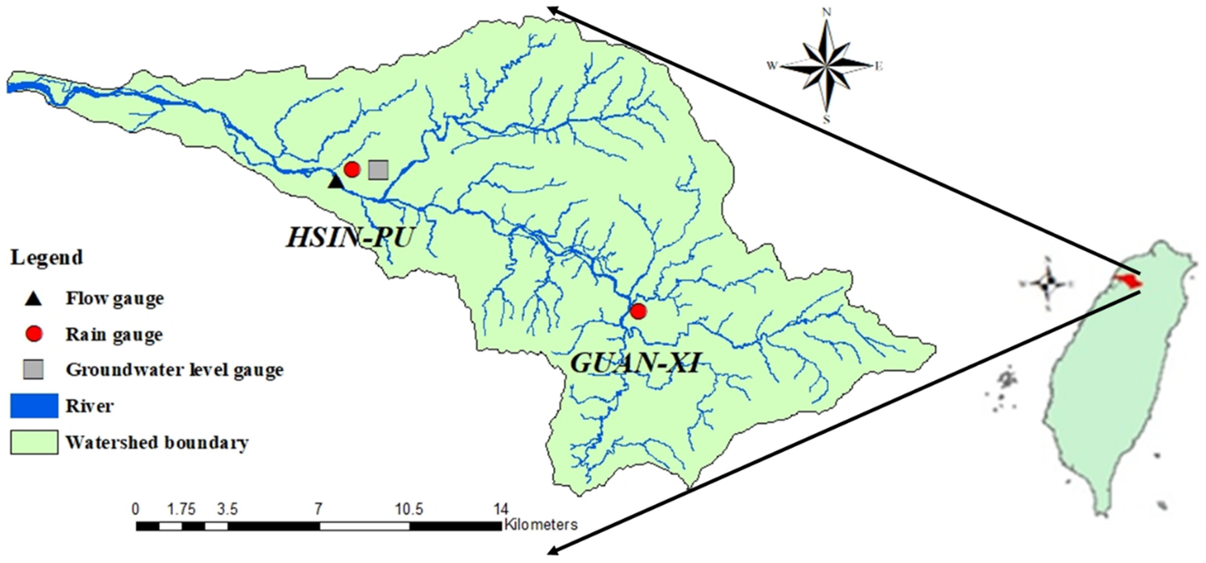
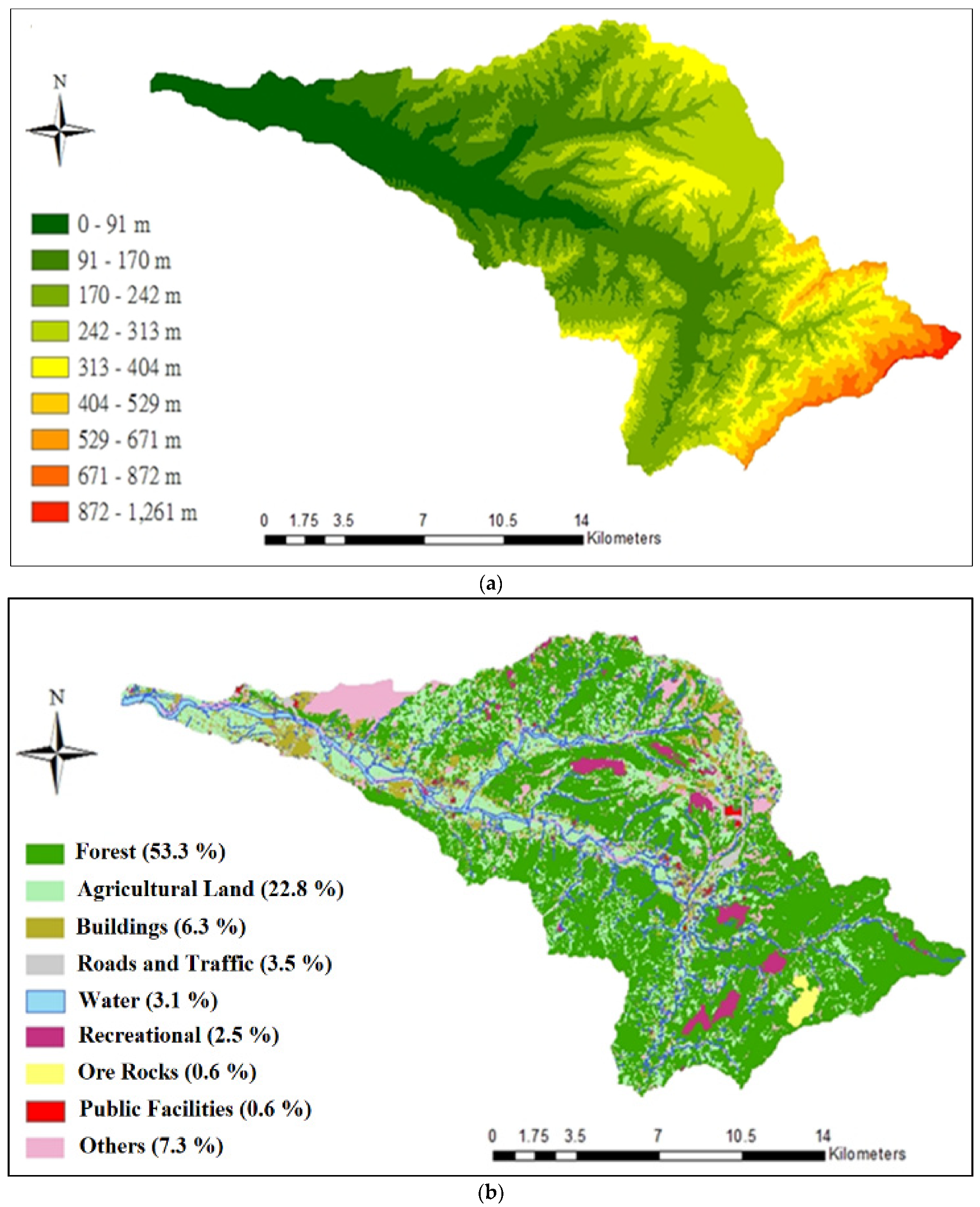
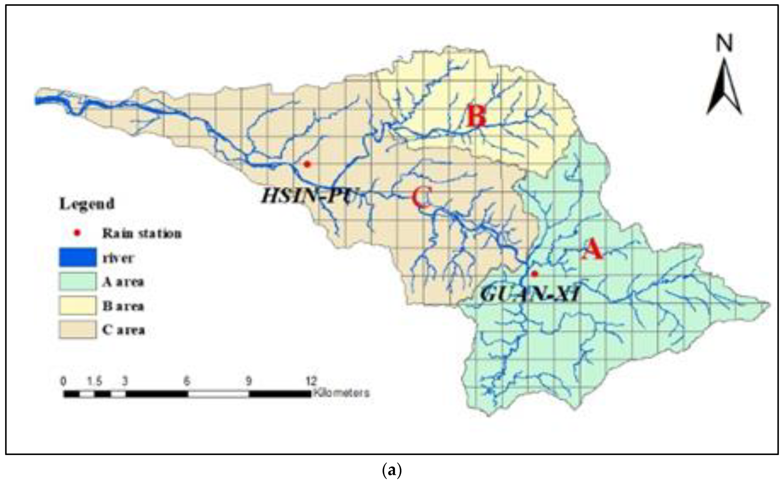
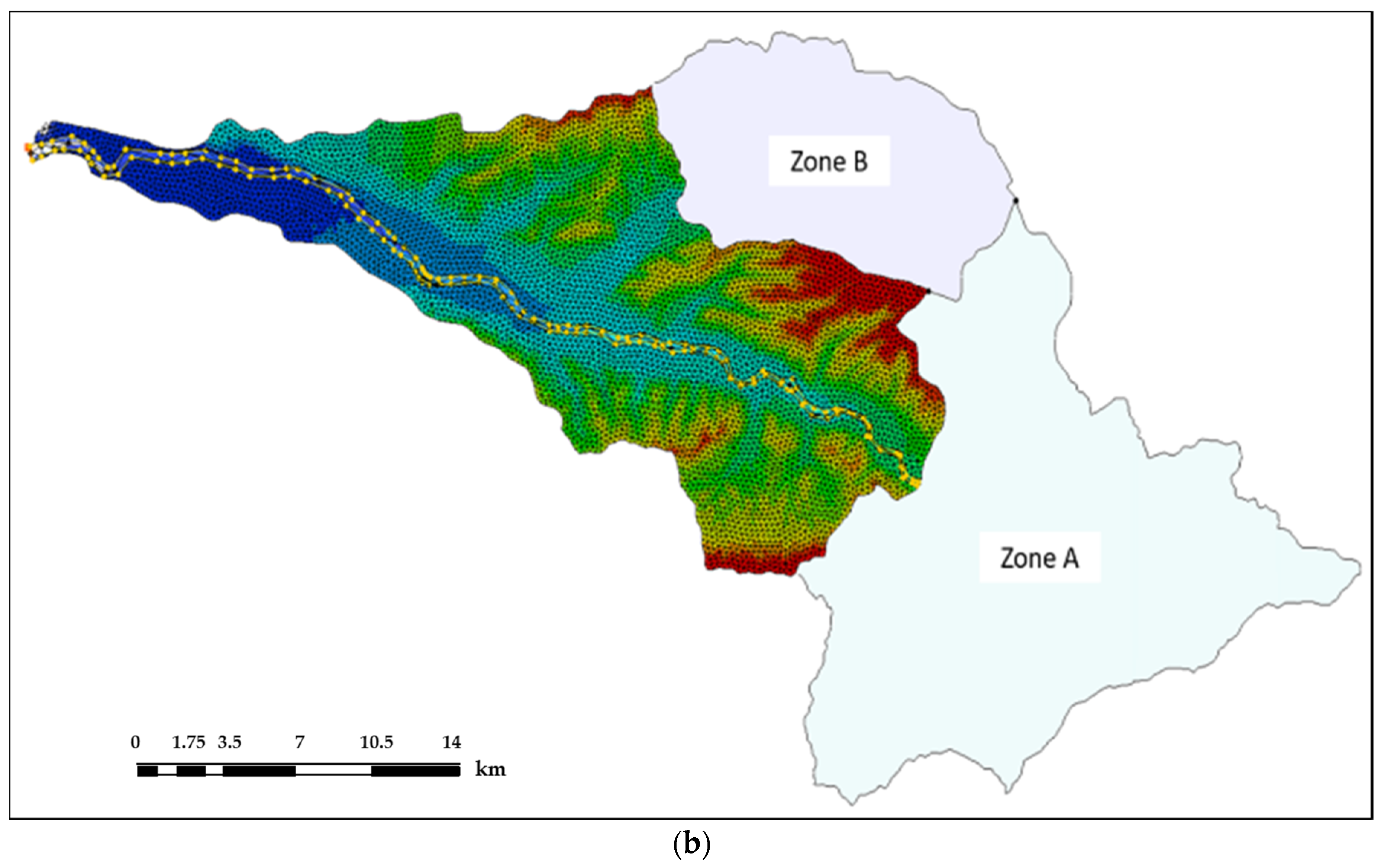
2.1. Study Area Description

The study area is Fèngshān River Basin (Figure 1), which covers Hsinchu County and Táoyuán City, Taiwan. It is one of the centrally managed rivers by the 2nd River Management Office, Water Resources Agency (WRA), and is the second-largest river in Hsinchu County. It originates from Guānxī Town, Jiānshí Township, and Táoyuán City Fùxīng in Hsinchu County. On the west side of Nèi Niǎo Zuǐ Mountain at the junction of the district, it is 1320 m above sea level. The Fèngshān River Basin is bounded by the Shèzi River, Lǎojiē River, and the upper reaches of Dànshuǐ River in the north, Tóuqián River in the east and south, and the Táiwān Strait in the west. The total length of the mainstream is about 45.5 km, and the drainage area is about 250.1 km². The average slope of the river is 1/225. Most of the basin area is hilly, and the flat land only accounts for 15.4% of the area, i.e., about 38.5 km² [13,15]. The annual runoff is 376 MCM, and the main tributaries are the Xiāolǐ River, Tàipíngwō River, and Xiàhéngkēng River.

In terms of climate, the Fèngshān River Basin has a subtropical climate, with humid summers and drier winters, with an average temperature of 22.5 °C. The average annual rainfall in the Fèngshān River Basin is 1608 mm, and the average number of rainy days per year is 167 days. Affected by monsoons and typhoons, the rainfall is concentrated in July, August, and September, with the monthly average rainfall ranging from 96 to 270 mm (Water Resource Agency; https://gweb.wra.gov.tw/HydroInfo/?id=Index (accessed on 1 January 2019)).

The monthly average river flows and water levels of the Fèngshān River at Xinpu bridge (121°3′56.268″ E, 24°49′32.959″ N) over the years (1970–2020) are shown in Figure 2. According to the WRA database, the average annual water level is 41.93 m, and the average annual flow is 9.62 cm. The average monthly flow and water level graph indicates that peak flows occur in the summer season while low flows in the winter season. The trend of high flow can also be used to deduce that the main rainy season lasts from June to September.

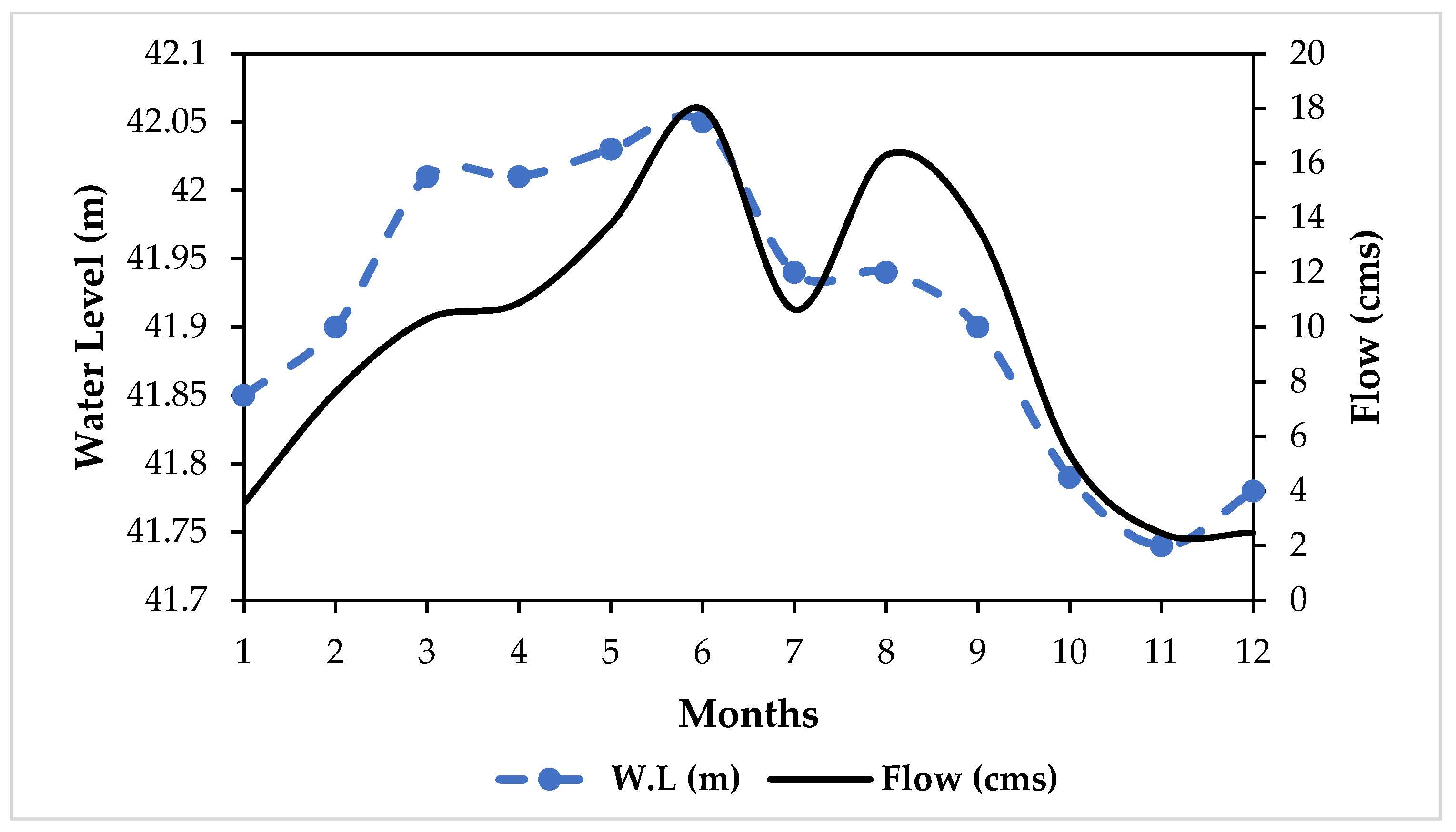
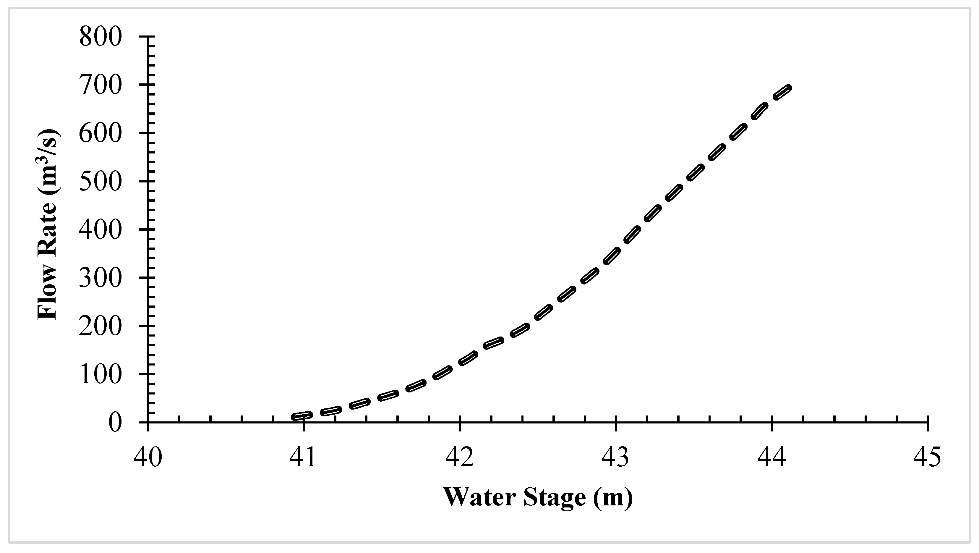
2.2. Data Required and Collection

The input data required for HEC-HMS and WASH123D modeling include topographical data (digital elevation model (DEM; 20 m resolution), landuse and soil type), hydrometeorological data (river stage, rain gauge, and radar rainfall), and river bathymetries data such as river cross-sections and Manning’s roughness. The data were collected from different government agencies, such as the topographic data were collected from the Center for space and remote sensing research (CSRSR), National Central University (http://www.csrsr.ncu.edu.tw/ (accessed on 1 January 2019)), National Land Surveying and Mapping Center (NLSC), Ministry of Interior, Taiwan (https://www.nlsc.gov.tw/En (accessed on 1 January 2019)) and Central Geological Survey (CGS), MOEA (https://www.moeacgs.gov.tw/main.jsp (accessed on 1 January 2019)). The hydrometeorological data were collected from Water Resource Agency (WRA) (https://gweb.wra.gov.tw/HydroInfo/?id=Index (accessed on 1 January 2019)) and the Central Weather Bureau (CWB) of Taiwan, and the National Severe Storms Laboratory (NSSL) of the National Oceanic and Atmospheric Agency (NOAA) of the USA.

The surface topography of the study area is mountainous, with a slope range from 5% to 35% and elevation ranges of 91 to 1261 m, as shown in Figure 3a. Landuse data from field investigations conducted by NLSC comprised nine coverage groups. It was investigated that 76% of the overall area is covered with agricultural and forest land, as shown in Figure 3b.

The rainfall data of two heavy rainstorms and two typhoon events (Mitag and Lekima) during 2019 were collected at the Hsin-Pu and Guan-Xi stations. The occurrence date, duration, and total rainfall amount for each typhoon are listed in

Table 1. Selected typhoons and rainy events were used in the study.

Event	Occurrence Date (Taipei Time)	Duration (h)	Total Rainfall (mm)	Maximum Water Level (m)
Plum Rain	16 May 0:00 to 18 May 23:00, 2019	72	137	44.09
Plum Rain	10 Jun 00:00 to 14 Jun 23:00, 2019	120	276	44.27
Lekima	7 Aug 00:00 to 10 Aug 23:00, 2019	96	198	43.27
Mitag	29 Sep 00:00 to 1 Oct 23:00, 2019	72	99	42.97

.

The high-resolution radar rainfall data (QPESUMS) from the Central Weather Bureau (CBW) of Taiwan were collected for the same rainfall and typhoon events for the quantitative rainfall forecasting. The CWB and NSSL of NOAA of the USA developed the Quantitative Precipitation Estimation and Segregation system using Multiples Sensors (QPESUMS) for radar rainfall data. This system comprises four weather Doppler radars which cover the whole of Taiwan and up to some range of adjacent ocean. The QPESUMS system provides corrected past 72 h to real-time Quantitative Precipitation Estimate (QPE) grid-based radar-derived rainfalls and 1 h Quantitative Precipitation Forecast (QPF). The correction of grid-based QPE radar rainfall is assured by integrating satellite, the radar network, and rain gauge data. The system covered the whole area of Taiwan (by 441 × 561 grid points) in the domain of (${118}^{°} \mathrm{E}–{123.5}^{°} \mathrm{E}$, ${20}^{°} \mathrm{N}–{27}^{°} \mathrm{N}$) with a spatial resolution of ${0.0125}^{°}$ (around 1.25 km) in both latitude and longitude directions with 10 min of temporal resolution since 2012. The study area domain has 15 × 30 grid points.

2.3. Flood Forecasting Model Reference to the Previous Study

In this study, the developed model of the previous study [13] was adopted for flood level forecasting. Hussain et al. (2021) worked on real-time correction of 1 h ahead flood forecasting using QPF data for the same study area. In the present study, we also developed a 1 h ahead flood-forecasting model with modification of QPF rainfall calculation and its application in the real-time correction process of flood forecasting. For this purpose, the previously developed model was adopted. Hussain et al. [13] used HEC-HMS and WASH123D watershed models for 1 h ahead flood level forecasting in Fèngshān River Basin. They presented a comprehensive step-by-step methodology for achieving 1 h ahead flood forecasting levels in Fèngshān River Basin. The conceptualization of the study area for model application as a preliminary explanation and configuration is shown in Figure 4, where the model’s geometry is divided into three zones. Zone A and B discharge simulations were performed using the HEC-HMS model, and then WASH123D was applied to simulate flood levels of zone C.

The difference in simulated hydrographs from observed hydrographs may be due to uncertainties in input data, differences between basin physics and model structure, model calibration, and catchment characteristics over time [13]. According to our understanding with respect to previous research, the uncertainty/error in radar rainfall is more important than is updated in this study by adopting a physical real-time correction approach with a goal of error prediction and correction, as shown in Figure 5 [13]. The approach was tested at cross-section 44 (Hsin-Pu Bridge) because of the availability of gauged data (observed water level).

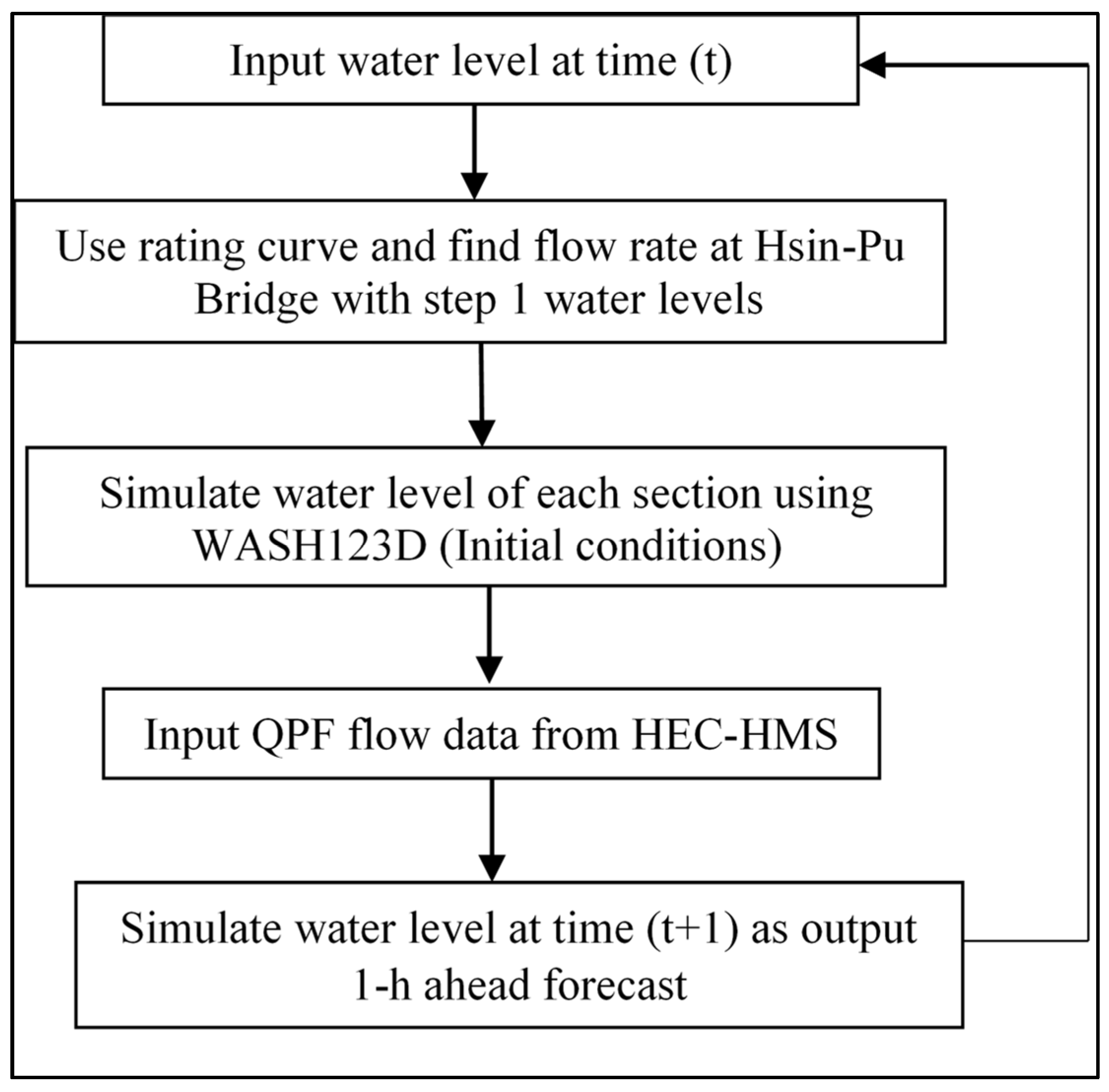
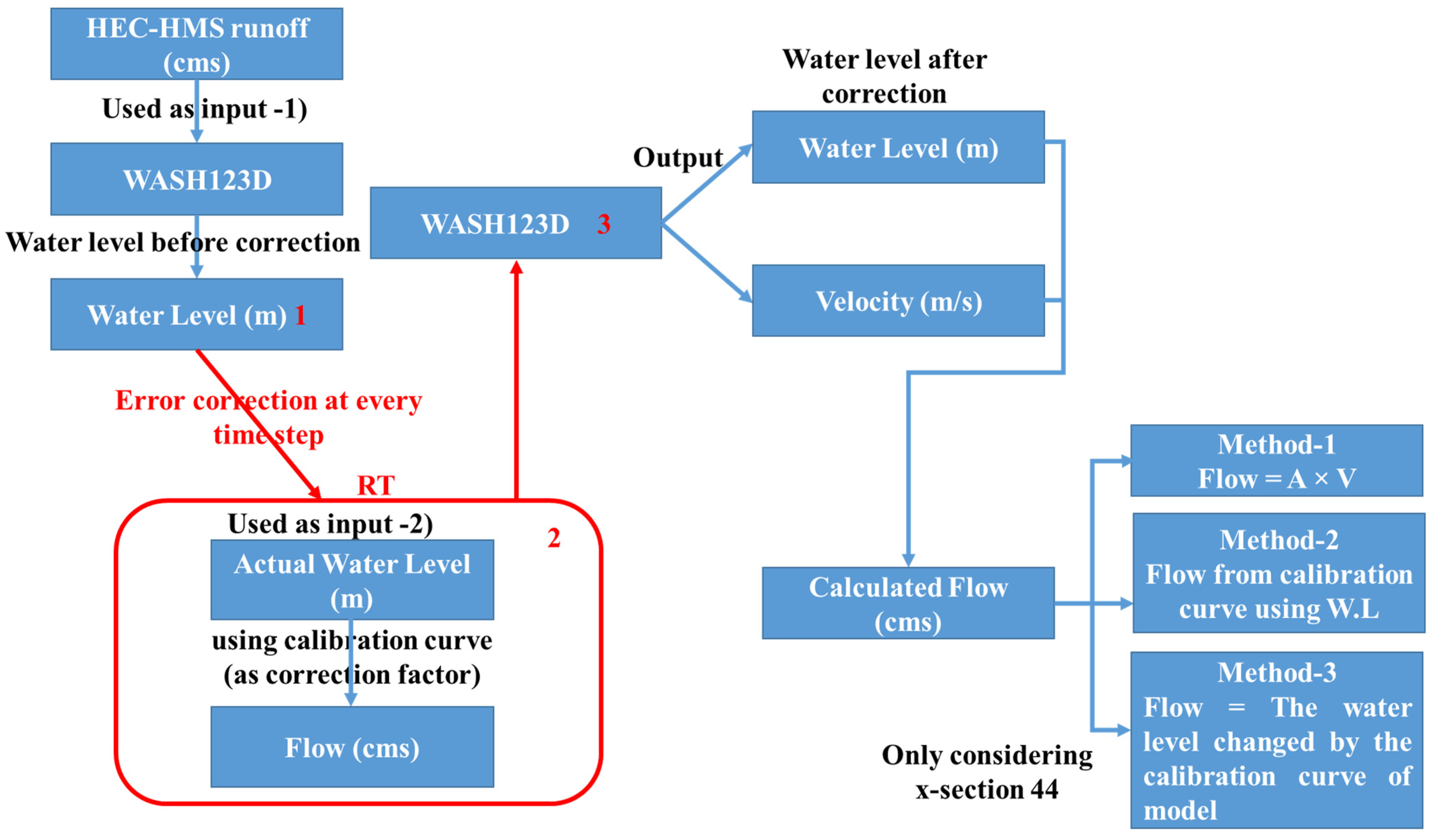
2.4. The Principle of Physical Real-Time Correction and Modifications in the Present Study for Flood Level Forecasting

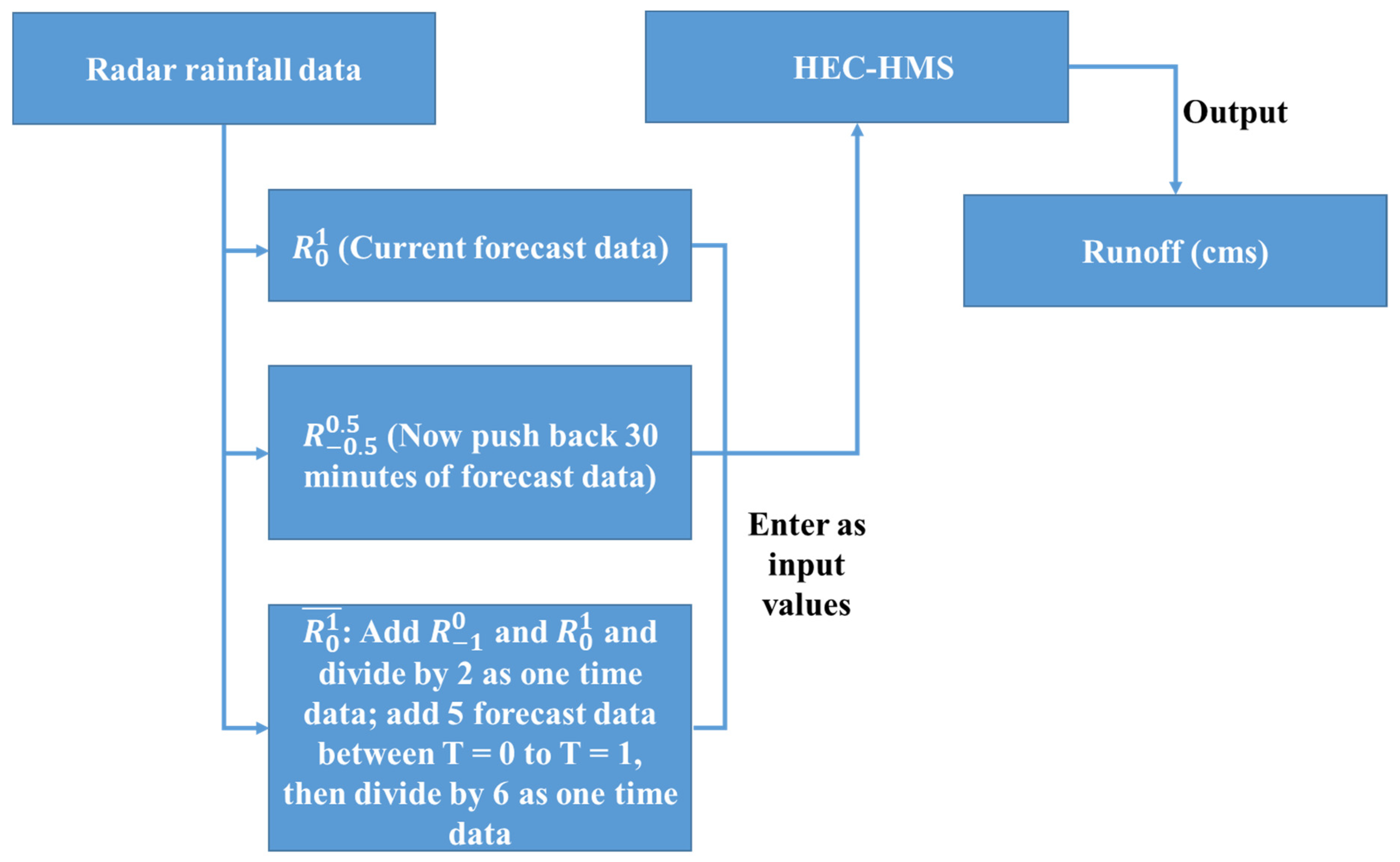
This study used the following one-hour radar rainfall prediction data (QPF) as input modeling environment (HEC-HMS and WASH123D) to conjecture 1 h ahead flood level forecasting. Hussain et al. [13] also predicted the same, but the obtained results were not satisfactory for all selected typhoon events because QPF data have certain errors. The results indicated large error prediction in QPF data might be because QPF needs to use maximum echo data with a 10 min update cycle by grids. At the same time, the selected typhoons have characteristics of thunderstorms with a dramatic change in rainfall intensity within short durations. These characteristics of typhoons make the QPESUMS system unable to capture these changes [13] fully. Using QPF data to fully capture the amount and timing of flood forecasting levels looks challenging due to available input and uncertain errors. Thus, error correction method called physical real-time error correction (RT) is adopted to improve the effectiveness of the flood warning system [13].

In the original forecasting method [13], only a set of initial water level data and base flow were input at the start time. Then, QPF data were input to calculate the water level value. When the model wants to calculate the water level at the next moment, the simulation value at this moment will be used as the starting data to start the calculation. In this method, the model’s error and the estimated error of the QPF itself accumulated. Therefore, this study improved the RT correction approach of Hussain et al. [13] by adopting the following methodology principle. The correction method substitutes the real-time observed water level into the model to eliminate accumulated errors and predict the water level at the next moment. However, there are 82 river sections in this model, but observational water level data are available in the 44th section (Hsin-Pu Bridge). The only correction of the water level of this section may cause unreasonable changes in the water level of all other sections (Figure 6). Therefore, it is necessary to make corrections to all river sections. In this study, base flow conditions are used as input into WASH123D to simulate the water level of section 44, and the calibration curve (stage-discharge relationship) is drawn, as shown in Figure 7. Using this relationship, the initial flow rate is obtained and put into WASH123D to find the water level of each section as the initial water level data, and enter the QPF at the 1st time step to calculate the water level at the next time step. Therefore, the correction of QPF is also important to simulate runoff using HEC-HMS, which will make the predicted water level the next step closer to the actual water level observation value [13].

The following three methods were adopted to correct the QPF data to predict water level at time step t = 1 (Figure 8).

Method 1: Direct input of QPF forecast data ($R_0^1$) of time step t = 0.

Method 2: Take time step t = −0.5, i.e., QPF rainfall forecast data ($R_{-0.5}^{ 0.5}$) in the first half of the time.

Method 3: The forecasted rainfall data ($R_{-1}^0$, $R_{-5/6}^{1/6}$, $R_{-1/3}^{1/3}$, $R_{-1/2}^{1/2}$, $R_{-2/3}^{2/3}$, $R_{-1/6}^{5/6}$, $R_0^1$) of 7 times between t = −1 and t = 0 was processed as QPF input value at t = 0 in a trapezoidal way:

We used the following steps to process the data and finally achieved Equation (1).

(a)

first, add up the rainfall forecast data ($R_{-1}^0$, $R_0^1$) of head and tail (t = 0 and t = 1) and divide by two as the data at one time,

(b)

add up every 10 min of rainfall forecast data between t = 0 and t = 1 i.e., ($R_{-5/6}^{1/6}$, $R_{-1/3}^{1/3}$, $R_{-1/2}^{1/2}$, $R_{-2/3}^{2/3}$, $R_{-1/6}^{5/6}$), and divided by 6 to obtain the QPF input value ($\overline{R_0^1}$) at time step t = 0.

$$\overline{R_0^1}=\left[\left(\frac{R_{-1}^0+R_0^1}{2}\right)+\left(\frac{R_{-5/6}^{1/6}+R_{-1/3}^{1/3}+R_{-1/2}^{1/2}+R_{-2/3}^{2/3}+R_{-1/6}^{5/6}}{6}\right)\right],$$

(1)

where, $R_{-1}^0$ is the QPF rainfall forecast data at t = 0 generated when t = −1, and $R_0^1$ is the QPF rainfall forecast data for the next hour generated at t = 0. $R_{-5/6}^{1/6}$~$R_{-1/6}^{5/6}$ are generated every ten minutes between t = −1 and t = 0, respectively. The QPF rainfall forecast data for the next hour starting at t = −1, forecast data generated at 10, 20, 30, 40, and 50 min. The step-by-step approach to calculating the QPF rainfall forecast is shown in Figure 8.

After calculating the QPF data, the values are used as input in HEC-HMS to obtain runoff. Then we run WASH123D to simulate and forecast flood levels during selected rainfall and typhoon events. We adopted the physical real-time correction process (RT), as shown in Figure 9, to correct the flood levels. The performance of the model was accessed using four measures such as coefficient of determination (CC), the root means square error (RMSE), the peak water level error (PE), and the peak time error (PTE). The details of these measures are provided in Hussain et al. [13].

In order to verify the influence of real-time physical correction on flow by WASH123D, the mass balance approach was used to calculate flow. Since there is only one water level measuring station (Hsin-Pu Bridge) in the study area, we adopted the following three methods (Figure 9) to calculate the flow and used them to evaluate the flow change after the model is instantly corrected by real-time physical correction. Out of 82 river sections, only the 44th section has to measure data on the water level, so the 44th section was used as a reference.

Method 1: Calculate the wetted cross-sectional area of each section with the predicted water level simulated by WASH123D multiplied by flow velocity.

Method 2: Convert the predicted water level simulated by WASH123D into flow through the calibration curve used in the model.

Method 3: Convert the water level measurement value obtained by the actual observation of the station into the flow rate through the calibration curve of the model.

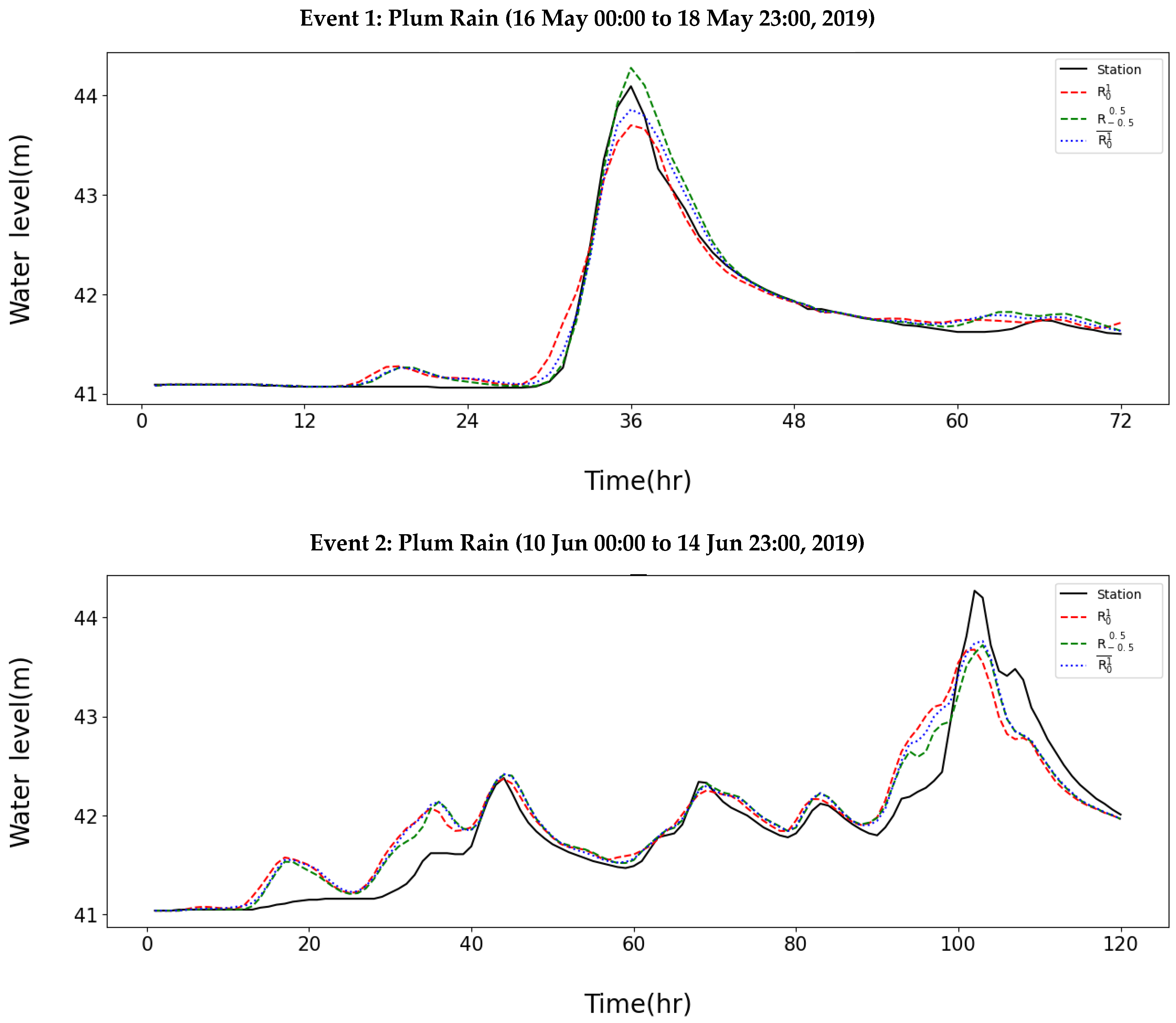
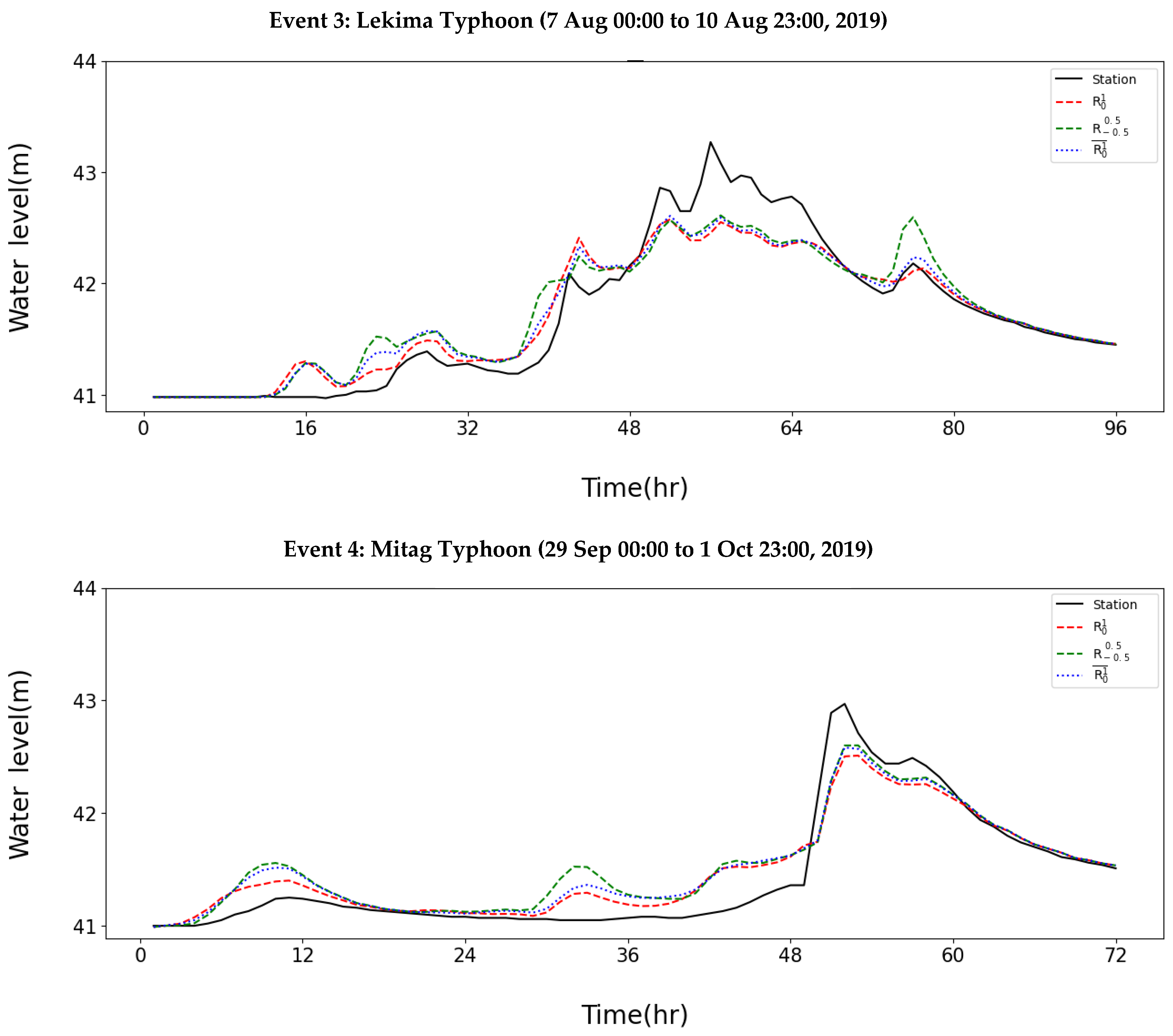
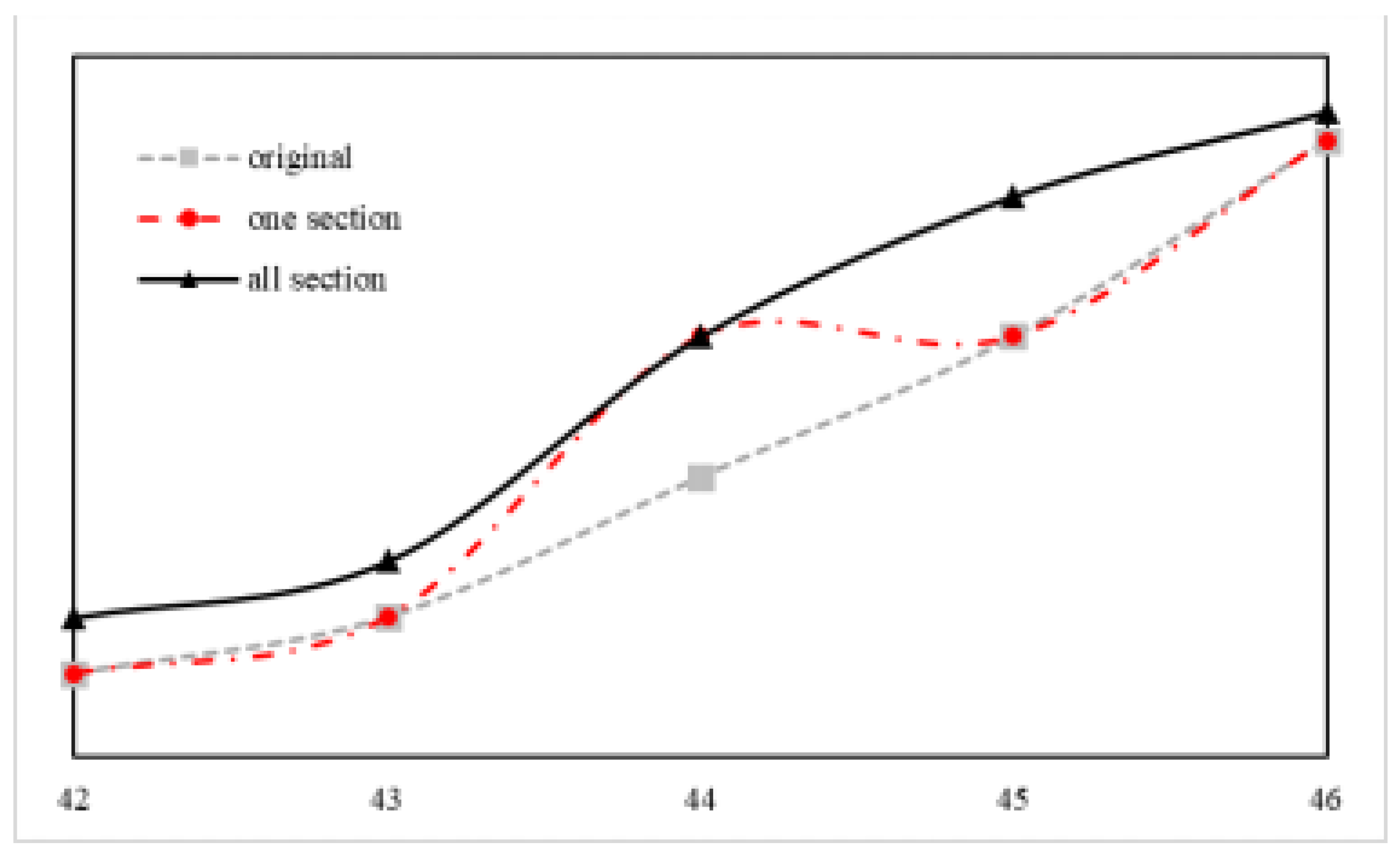
3. Results and Discussion

After calculating the radar rainfall of QPF according to the three methods ($R_0^1$, $R_{-0.5}^{0.5}$, $\overline{R_0^1}$) as described in Section 2.4, and inputs it into the model to simulate the water level (Figure S1) as shown in supplementary material. The solid black line in the rainfall and predicted water level diagrams represents the actual measured value of the station, and the red dashed line represents the predicted result of the $R_0^1$ rainfall using the calculated water level; the green dashed line represents $R_{-0.5}^{0.5}$ rainfall using the calculated water level predictions; the blue dashed line represents $\overline{R_0^1}$ rainfall using calculated water level predictions. The difference between the water level prediction results simulated by the three methods and the actual water level observation were analyzed to select an appropriate method that can be used to calculate the water level prediction results of radar rainfall. Figure S2 in supplementary material shows the water level simulation results after real-time correction (RT) with the direct simulation (without real-time correction) for calculated rainfall using these three methods. The direct simulation initial input parameters were obtained from the calibration curve only at the first time step and for the subsequent time step; results were directly simulated without adding corrections. The solid black line represents the actual measurement value of the station, the red dotted line represents the water level prediction result of RT correction, and the green dotted line represents the water level prediction result of direct simulation (without correction).

The results obtained were encouraging but not satisfactory (Figure S1). Therefore, QPF forecasted flood levels were immediately corrected using modification/correction and real-time correction techniques (Figure S1). The model results provide a reasonable river stage hydrograph during all rainfall events and reveal a good resemblance between observed and simulated river stages using the WASH123D model. The comparative analysis of the obtained results with observations was performed using statistical measures (

Table 2. Relative comparison of error amount between direct simulation and QPF correction methods for all rainfall events.

Statistical Parameters	Direct Simulation				Real-Time Correction
	Event 1	Event 2	Event 3	Event 4	Event 1	Event 2	Event 3	Event 4
	Method 1
CC	0.85	0.65	0.69	0.41	0.99	0.93	0.96	0.96
RMSE (m)	0.54	0.57	0.58	0.51	0.12	0.28	0.21	0.18
PE (m)	−0.65	−0.83	−0.95	−0.93	−0.39	−0.59	−0.69	−0.46
ETp (h)	0	−2	−14	−1	0	0	−4	1
	Method 2
CC	0.91	0.74	0.63	0.41	0.99	0.96	0.94	0.94
RMSE (m)	0.45	0.5	0.58	0.52	0.11	0.23	0.24	0.21
PE (m)	0.01	−0.8	−0.42	−0.82	0.19	−0.55	−0.66	−0.37
ETp (h)	0	1	20	0	0	1	1	1
	Method 3
CC	0.9	0.73	0.68	0.44	0.99	0.95	0.96	0.96
RMSE (m)	0.45	0.51	0.56	0.5	0.09	0.25	0.21	0.19
PE (m)	−0.39	−0.76	−0.97	−0.84	−0.23	−0.5	−0.66	−0.39
ETp (h)	0	1	20	0	0	1	−4	0

). The results obtained using QPF data (direct simulation; Figure S2) were not according to expectation because QPF data itself have certain errors as represented by statistical performance evaluation indices. It was observed that QPF without correction showed over and under prediction fluctuations in all events. It was analyzed that all events showed an RMSE range of 0.51 to 0.58 m with CC = 0.41–0.85 for method one, indicating a poor correlation between simulated and observed water levels except for event one with CC = 0.85 (Table 2). The poor correspondence between peak rainfall intensity and peak water level with a time lag (ETp) of almost −1 to −14 h and peak error (PE) −0.65 to −0.95 m (maximum error for event three) indicated that WASH123D direct simulation did not fully capture the rising, peak and receding limbs of water level patterns (Table 2; Figure S2). The direct simulations for all three methods showed inconsistencies with observations indicated by CC, RMSE, ETp, and PE statistical parameters (Table 2); it is difficult to use QPF information directly for flood forecasting because QPF predictions did not provide correct information related to timing and amount of flood peak. At the same time, QPF is considered an important variable for the early warning system for floods. Accurate prediction of the peak level, timing, and location are challenging tasks for flood warning authorities. Therefore, this study introduced three different methods to correct and calculate QPF data to forecast flood levels and applied a real-time error correction method to improve flood warning effectiveness.

Table 2 summarizes that the corrected results are improved compared with QPF direct simulation. The results are good as identified by the values of CC and RMSE but relatively poor in terms of PE and ETp for event three. It was analyzed that the forecasting and observations are in excellent agreement and follow the patterns. The CC raised above 0.93, and RMSE is below 0.28 m among all events using all three methods of QPF calculation. The model somehow underestimated every event’s flood stage forecasting (time and occurrence), whereas low magnitude water levels were accurately predicted. The comparison between prediction and observations followed the pattern, but the model was limited to capturing the flood peak time and peak level; however, the model represents the overall hydrology (Figure S1). The simulated hydrograph patterns are quite close to the observed data and reasonably capture the timing of peak flood levels, as shown in Figure S1. However, a small acceptable error of PE may be due to QPF prediction itself containing too much error. The prediction results obtained using real-time correction indeed reasonably reflect the hydrological changes within the entire events, whether in ascending, peak, or receding sections of stage hydrograph, and handsomely encountered the errors of forecasted flood levels simulated with the help of QPF rainfall as input data. Keeping in view the high prediction reliability with efficient correction results, a physical real-time correction approach using the numerical model (WASH123D) proved an accurate novel modeling during typhoon events for peak and low magnitude flood stage forecasting. This approach is helpful for early flood warning and indicates that the watershed’s physical characteristics are very important for flood level forecasting.

Since the QPF rainfall forecast data come from the radar echo epitaxy method, there is a certain error. Theoretically, to predict the water level in the next hour, the next hour of forecasted rainfall ($R_0^1$, $R_{-0.5}^{0.5}$) of a single moment should be used. When there is a large error in the forecast data, it will directly affect the accuracy of the water level forecast. Therefore, it is hoped that the $\overline{R_0^1}$ method adopted can reduce the influence caused by extreme values. As can be seen from Figure 10 that the simulated peak water level results of the calculated $\overline{R_0^1}$ rainfall (method three) is closer to the actual value than method one. Overall, the simulated water level is roughly in the middle of method one and method two during the rainfall pattern of $\overline{R_0^1}$. Event one is relatively simple, and the difference between the three methods is more obvious. The flood peak water level results simulated by the three methods of event three are all lower than the actual value, and the rainfall decrease rate is too fast, which leads to an excessive underestimation of the simulated water level, which is presumed to be caused by the error of the radar prediction data itself. From the statistical results of four events (Table 2), the flood peak error of simulation results is relatively low. The flood peak water level error is 0.16 m of method one–event one is smaller than event two and four, 0.7–0.8 m, respectively. According to the comparison of methods of the rainfall events, method three is better than the other two methods as represented by the highest correlation coefficient and lowest value of root mean square error (Table 2). Overall, no matter which calculation method is used, the predicted value of the simulated water level corrected by real-time physical correction is close to the actual measured value and better than the uncorrected simulations. It can be seen from Table 2 that before correction, the CC is low, the RMSE and PE are high, and the ETp difference is not large, while after the real-time correction, the CC is above 0.9, the RMSE is 0.1–0.2 m, and PE tends to decrease in most cases.

Comparison of Flow before and after RT Correction

The calculated results for the comparison of flow rate before and after RT correction are shown in

Table 3. Comparison of calculated flow rate before and after RT correction.

Event	Rainfall Duration (h)	Direct Simulated Flow Rate (m3/h) before RT	Real-Time Correction of Flow Rate (m3/h) after RT	Difference between before and after RT (m3/h)	Percentage Difference
1	72	7.46 × 104	7.48 × 104	196.63	0.26%
2	120	7.78 × 104	7.80 × 104	145.61	0.19%
3	96	7.54 × 104	7.54 × 104	22.49	0.03%
4	72	7.06 × 104	7.06 × 104	11.29	0.02%

. After the RT real-time correction of the four rainfall events, the change in the overall flow rate is not large, and the total flow rate after real-time correction is only about 0.02% to 0.3% more than the directly simulated total flow rate. The low percentage difference was calculated in event three and event four, i.e., less than 0.03%, which may be due to the low intense rainfall of these events. The observed intensity of rainfall for these events was less than 15 mm/h, while for events one and two, the observed intensity was up to 35 mm/h. This variation in results indicated that rainfall events’ duration and characteristics impact the flood forecasting flow rate.

Table 4. Comparison of total calculated flow by different methods with total flow from radar rainfall + base flow for each event of WASH123D (MCM: million cubic meters).

Event	Total Flow (MCM)			Total Flow (MCM)	Percentage Difference with Respect to both Flows
	Method 1	Method 2	Method 3	Radar Precipitation + Base Flow	Method 1	Method 2	Method 3
1	40.6	27.84	26.67	31.52	29%	−12%	−15%
2	88.38	60.38	56.5	69.58	27%	−13%	−19%
3	46.95	33	36.03	30.67	53%	8%	17%
4	22.59	16.49	15.95	22.68	0%	−27%	−30%

compares the flow calculated by three different methods and the mass balance method of radar precipitation + base flow of four rainfall events. It can be seen that the error of method one is higher than that of the other two methods except for event four, while the error of method two is the smallest. Method three is converted from the actual water level through the model calibration curve. It is close to the result of method two, where the water level is used to calculate the flow, which is theoretically closer to the flow simulated by the model. Therefore,

Table 5. Comparison of total RT calculated flow by different methods with direct simulation flow for each event of WASH123D (MCM: million cubic meters).

Event	RT Simulation (MCM)		Direct Simulation (MCM)		Percentage Difference
	Method 1	Method 2	Method 1	Method 2	Method 1	Method 2
1	40.6	27.84	27.78	18.84	32%	32%
2	88.38	60.38	71.87	49.32	19%	18%
3	46.95	33	27	20.2	42%	39%
4	22.59	16.49	18.22	13.81	19%	16%

compares calculated flow with RT and direct simulation using method one and method two for all four events. From Table 5, it can be seen that method one slightly overestimated the flow more than the other two flow calculation methods in most cases. When considering the corrected event flow as a true value after real-time correction, the flow change is about 16% to 42% of the direct simulation. This is due to many uncertainties in the calibration curve itself and is considered acceptable as flow change is more than direct simulation, which is considered safe in case of a flood warning [13].

4. Conclusions

This study introduced three different methods of radar rainfall calculation to reduce the error in flood forecasting caused by QPF radar rainfall forecast data. The flood forecasting has been performed in Fèngshān River Basin, Taiwan using the WASH123D hydrology model for four rainfall/typhoon events. The simulated results were corrected using a physical real-time correction technique and compared with direct simulation without correction for all three QPF calculation methods. According to model performance evaluation criteria, the third method of QPF calculation flood peak error was the lowest in all three methods indicating better results for flood forecasting. It can be used for flood early warning systems. The impact of the real-time correction technique was assessed using mass balance analysis. It was found that flow change is between 16% and 42% from direct simulation, indicating overestimation, which is just on the safe side in case of a flood warning. However, the impact of the real-time physical correction on the water level is in a reasonable range. Still, QPF rainfall correction/calculation is more important to obtain accurate results for flood forecasting. Therefore, the application of real-time correction to correct the model water level has certain credibility for the water balance model. The adopted methodology is operational and recommended to use by the government in the future for early warning to reduce the flood impacts during typhoon events.

References

1. WMO. Manual on Flood Forecasting and Warning; WMO No. 1072; World Meteorological Organization: Geneva, Switzerland, 2011. [Google Scholar]
2. Jain, S.K.; Mani, P.; Jain, S.K.; Prakash, P.; Singh, V.P.; Tullos, D.; Kumar, S.; Agarwal, S.P.; Dimri, A.P.A. Brief review of flood forecasting techniques and their applications. Int. J. River Basin Manag. 2018, 16, 329–344. [Google Scholar] [CrossRef]
3. Corral, C.; Sempere-Torres, D.; Revilla, M.; Berenguer, M. A semi-distributed hydrological model using rainfall estimates by radar: Application to Mediterranean basins. Phys. Chem. Earth B 2000, 25, 1133–1136. [Google Scholar] [CrossRef]
4. Borga, M.; Degli Esposti, S.; Norbiato, D. Influence of errors in radar rainfall estimates on hydrological modeling prediction uncertainty. Water Resour. Res. 2006, 42, W08409. [Google Scholar] [CrossRef] [Green Version]
5. Cole, S.J.; Moore, R.J. Hydrological modelling using raingauge- and radar-based estimators of areal rainfall. J. Hydrol. 2008, 358, 159–181. [Google Scholar] [CrossRef]
6. Chiang, Y.M.; Chang, F.C. Integrating hydrometeorological information for rainfall-runoff modelling by artificial neural networks. Hydrol. Process. 2009, 23, 1650–1659. [Google Scholar] [CrossRef]
7. Lin, G.F.; Chou, Y.C.; Wu, M.C. Typhoon flood forecasting using integrated two-stage support vector machine approach. J. Hydrol. 2013, 486, 334–342. [Google Scholar] [CrossRef]
8. Yu, P.S.; Yang, T.C.; Chen, S.Y.; Kuo, C.M.; Tseng, H.W. Comparison of random forests and support vector machine for real-time radar-derived rainfall forecasting. J. Hydrol. 2017, 552, 92–104. [Google Scholar] [CrossRef]
9. Liu, Y.; Gupta, H.V. Uncertainty in hydrologic modeling: Toward an integrated data assimilation framework. Water Resour. Res. 2007, 43, W07401. [Google Scholar] [CrossRef]
10. Hostache, R.; Matgen, P.; Montanari, A.; Montanari, M.; Hoffmann, L.; Pfister, L. Propagation of uncertainty in coupled hydro-meteorological forecasting system: A stochastic approach for the assessment of the total predictive uncertainty. Atmos. Res. 2010, 100, 263–274. [Google Scholar] [CrossRef]
11. Wu, S.-J.; Lien, H.-C.; Chang, C.-H.; Shen, J.-C. Real-time correction of water stage forecast during rainstorm events using combination of forecast errors. Stoch. Environ. Res. Risk Assess. 2012, 26, 519–531. [Google Scholar] [CrossRef]
12. Wu, M.C.; Lin, G.F. The very short-term rainfall forecasting for a mountainous watershed by means of an ensemble numerical weather prediction system in Taiwan. J. Hydrol. 2017, 546, 60–70. [Google Scholar] [CrossRef]
13. Hussain, F.; Wu, R.S.; Wang, J.X. Comparative study of very short-term flood forecasting using physics-based numerical model and data-driven prediction model. Nat. Hazards 2021, 107, 249–284. [Google Scholar] [CrossRef]
14. Lohani, A.K.; Goel, N.; Bhatia, K. Improving real time flood forecasting using fuzzy inference system. J. Hydrol. 2014, 509, 25–41. [Google Scholar] [CrossRef]
15. Wu, R.S.; Shih, D.S. Modeling hydrological impacts of groundwater level in the context of climate and land cover change. Terr. Atmos. Ocean. Sci. 2018, 29, 341–353. [Google Scholar] [CrossRef] [Green Version]
Figure 1. Fèngshān River Basin location map.
Water 14 01866 g001
Figure 2. The monthly average river flows and water levels of Fèngshān River at Xinpu Bridge.
Water 14 01866 g002
Figure 3. (a) Digital Elevation Model of the year 2016, (b) Landuse classification map of Fèngshān River Basin.
Water 14 01866 g003
Figure 4. Conceptualization of the study area for model application, zones (A and B) in HEC-HMS and zone C in WASH123D (a) Mesh construction from radar grid points (b) grid constructions of WAH123D [13].
Water 14 01866 g004aWater 14 01866 g004b
Figure 5. Model set up for real-time physical correction, adopted from Hussain et al. [13].
Water 14 01866 g005
Figure 6. Demonstration of river section water level correction.
Water 14 01866 g006
Figure 7. Stage-discharge relationship at Hsin-Pu Bridge for base flow calculation.
Water 14 01866 g007
Figure 8. QPF rainfall calculation method.
Water 14 01866 g008
Figure 9. Physical real-time correction, a three-step approach, represented numbers 1 to 3 in red colour.
Water 14 01866 g009
Figure 10. Comparison of simulated water level results for event 1 to event 4 using R 0 1 , R 0.5 0.5 , R 0 1 ¯ rainfall methods.
Water 14 01866 g010aWater 14 01866 g010b