
Improving the Prediction of Soil Organic Matter in Arable Land Using Human Activity Factors

 , ,
, ,
Abstract
:1. Introduction
2. Materials and Methods
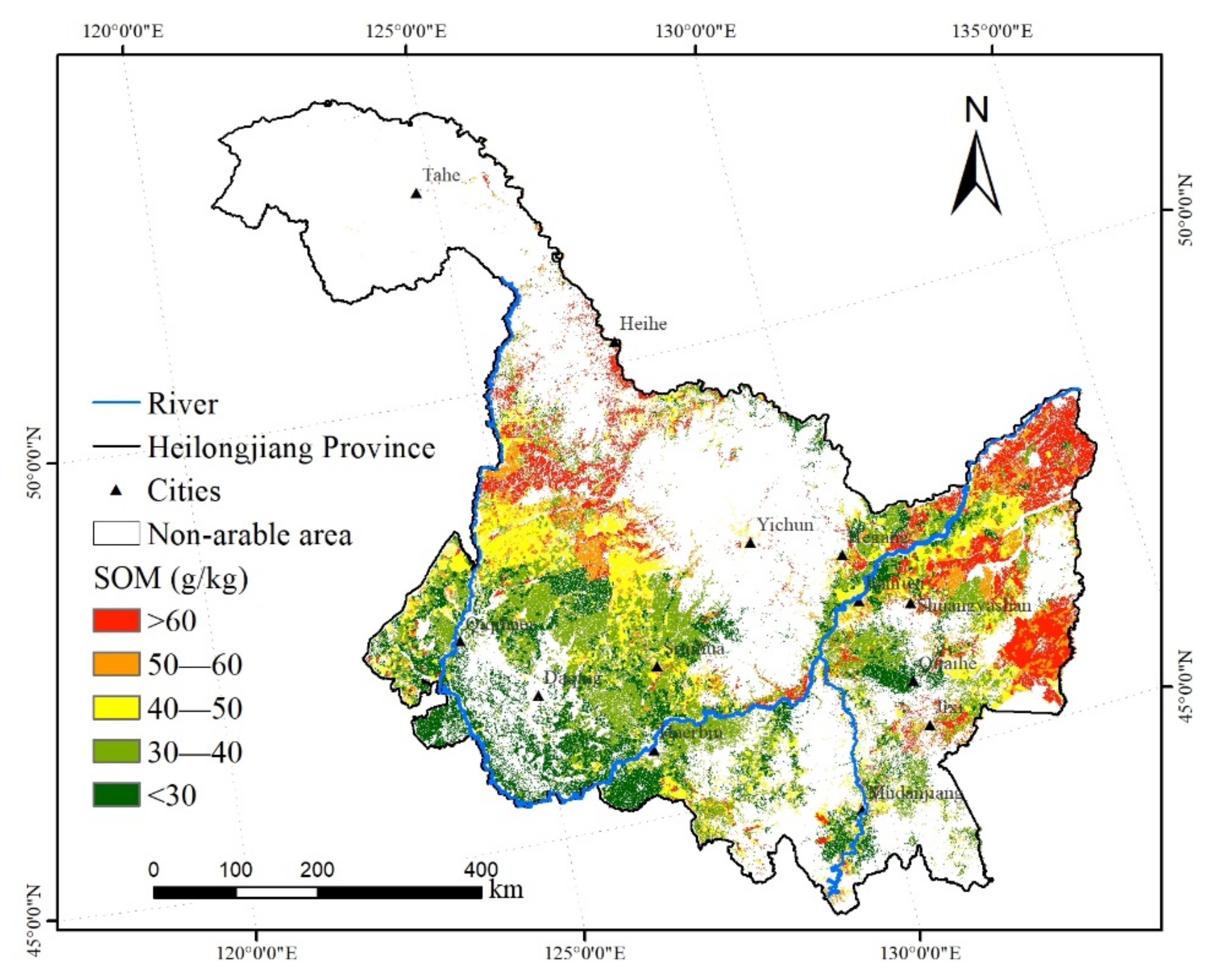
2.1. Study Area
2.2. SOM Data
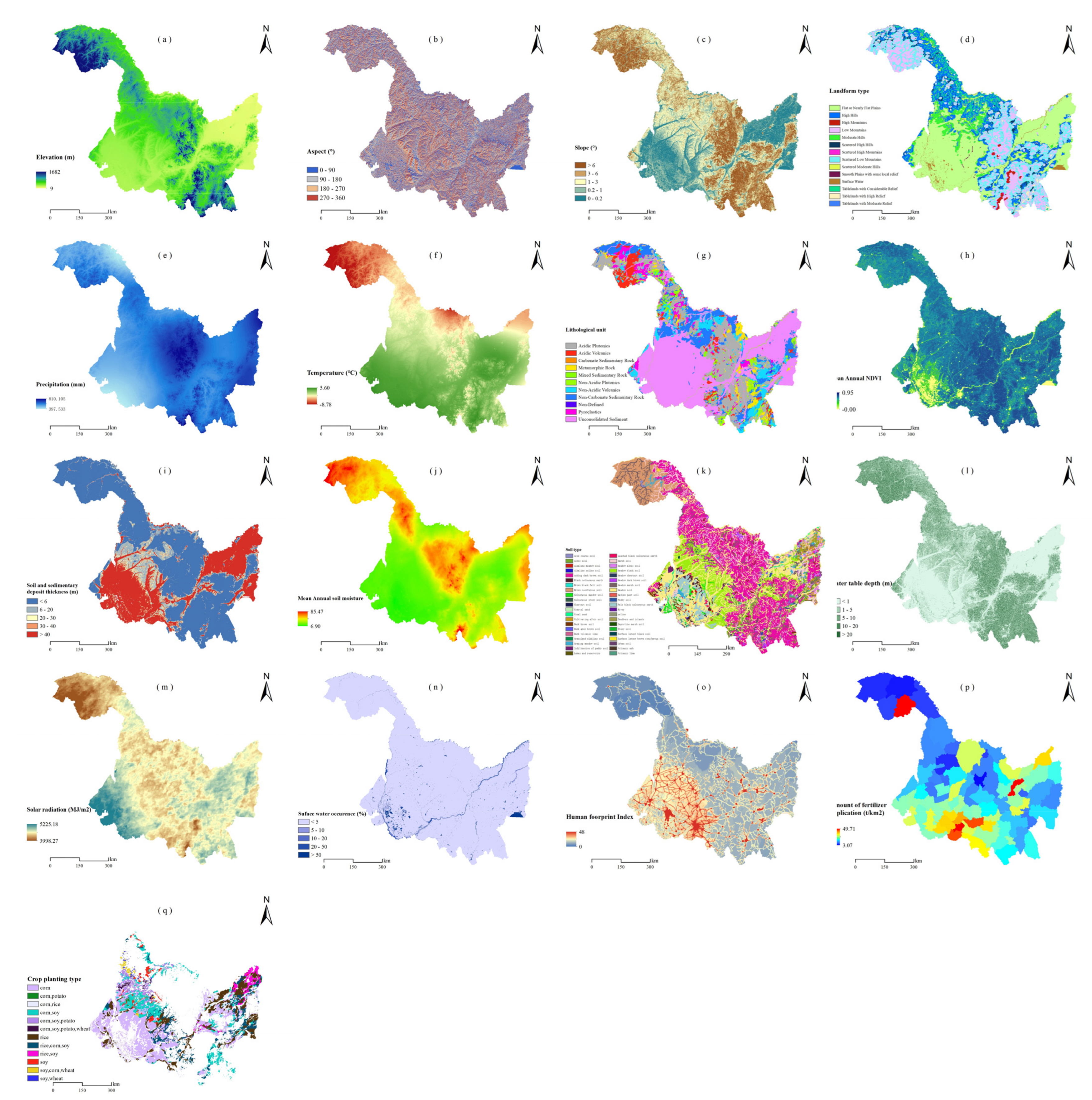
2.3. Covariates
2.4. Data Pre-Processing
2.5. Modeling and Evaluation
3. Results
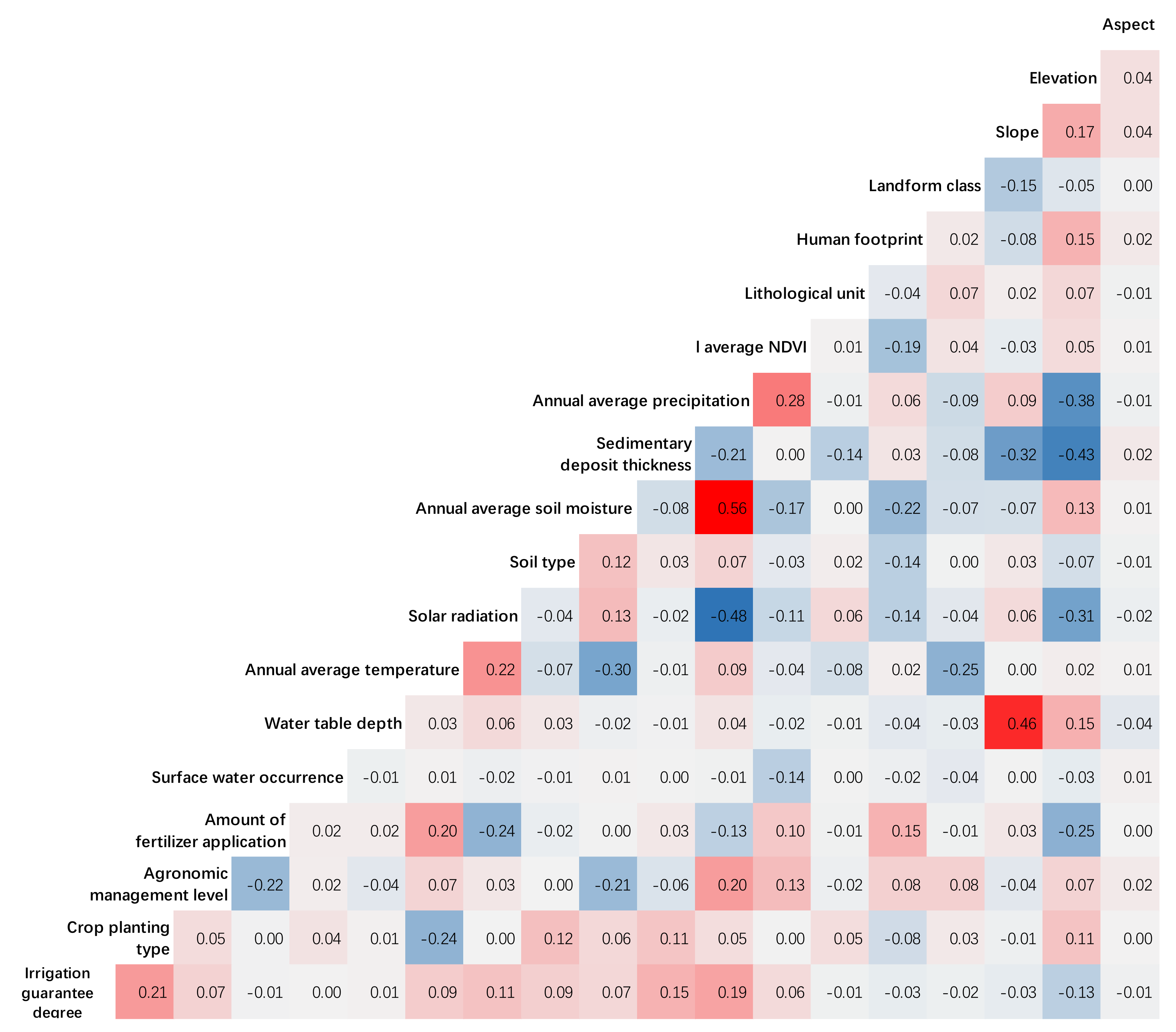
3.1. Feature Selection
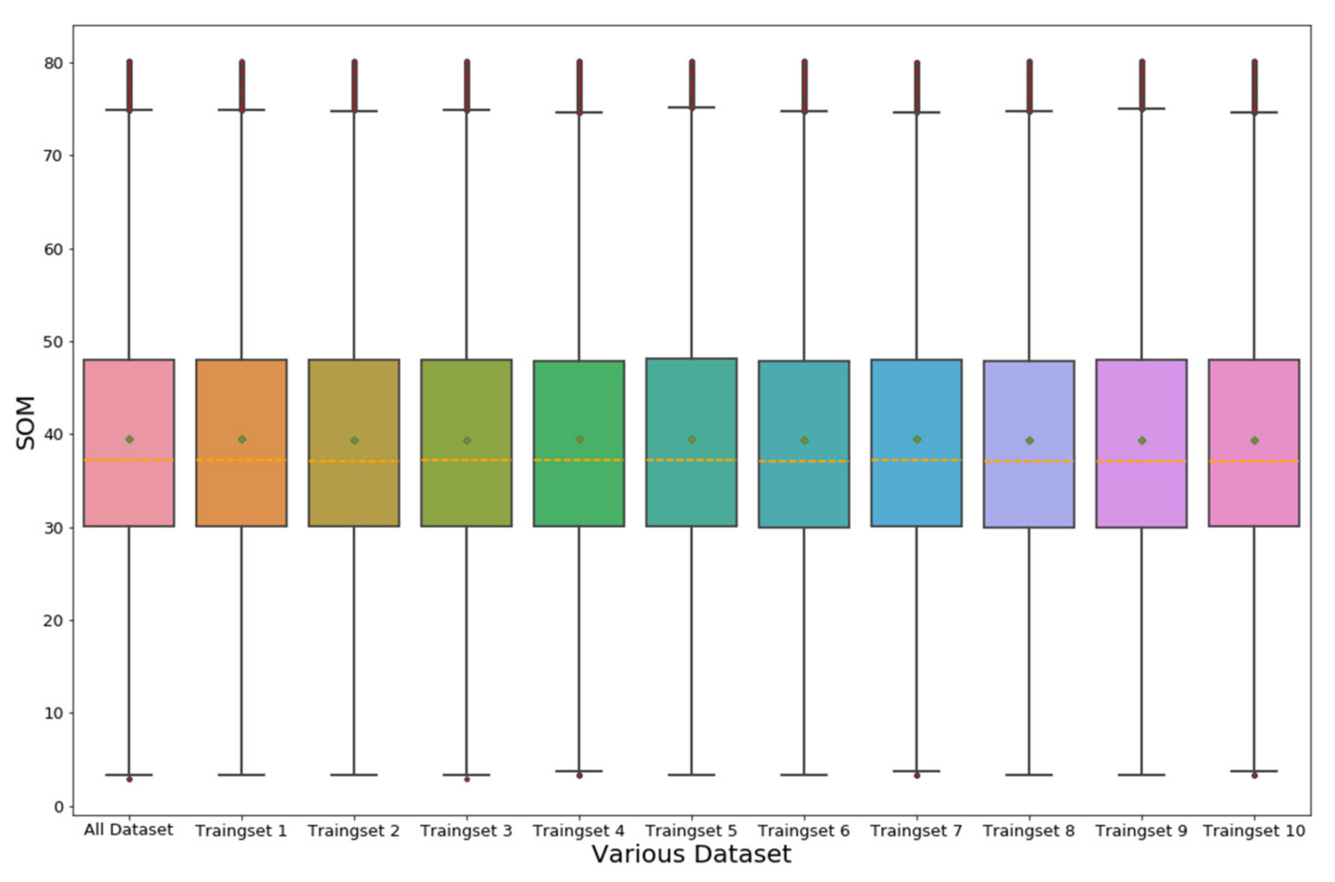
3.2. Descriptive Statistics
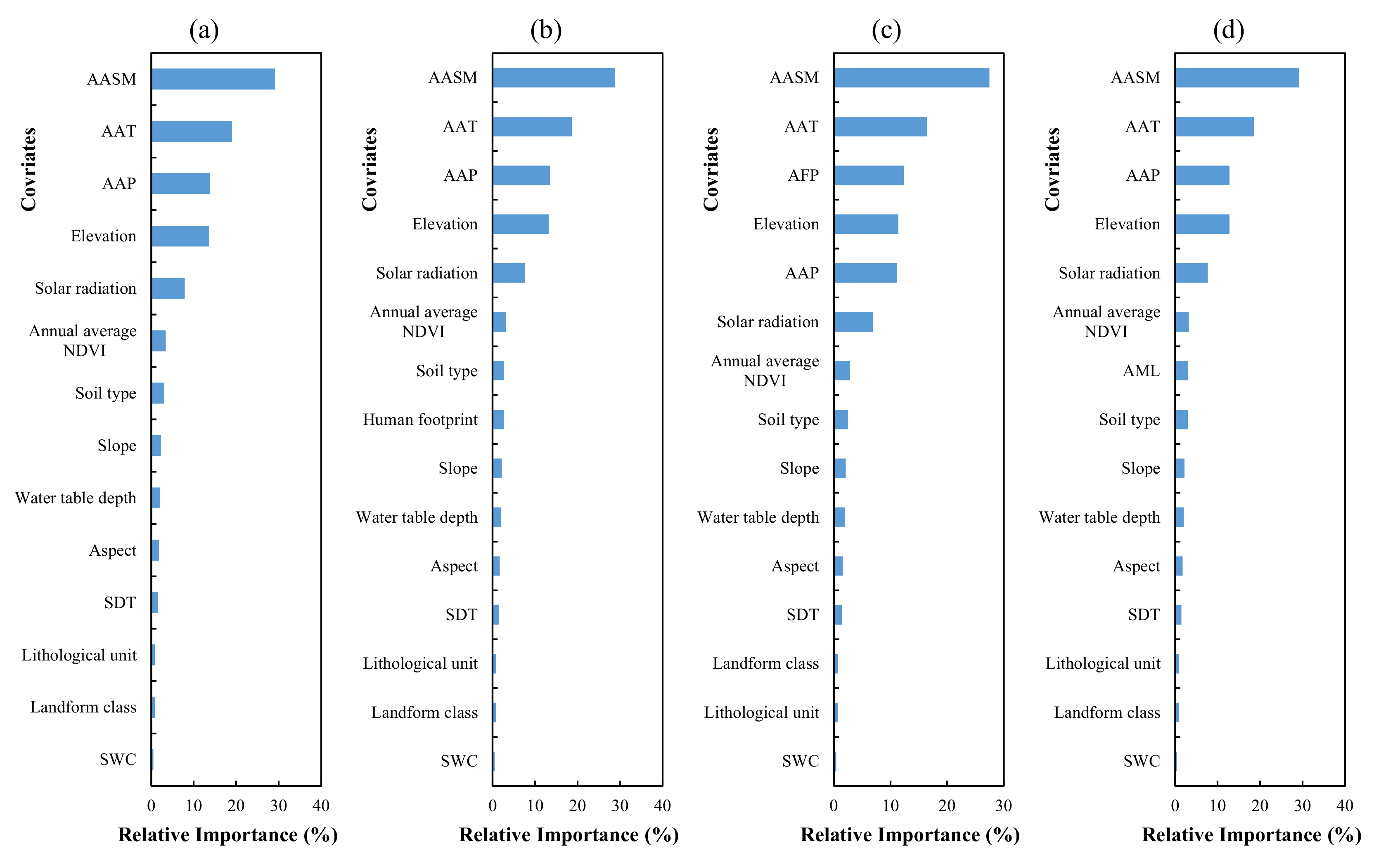
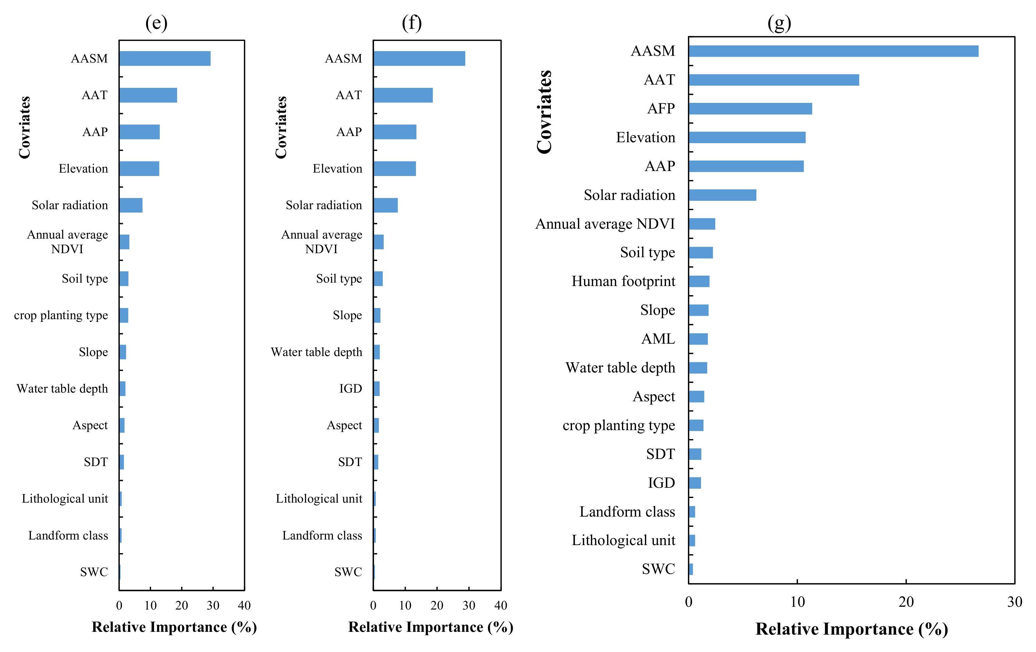
3.3. Covariate Importance
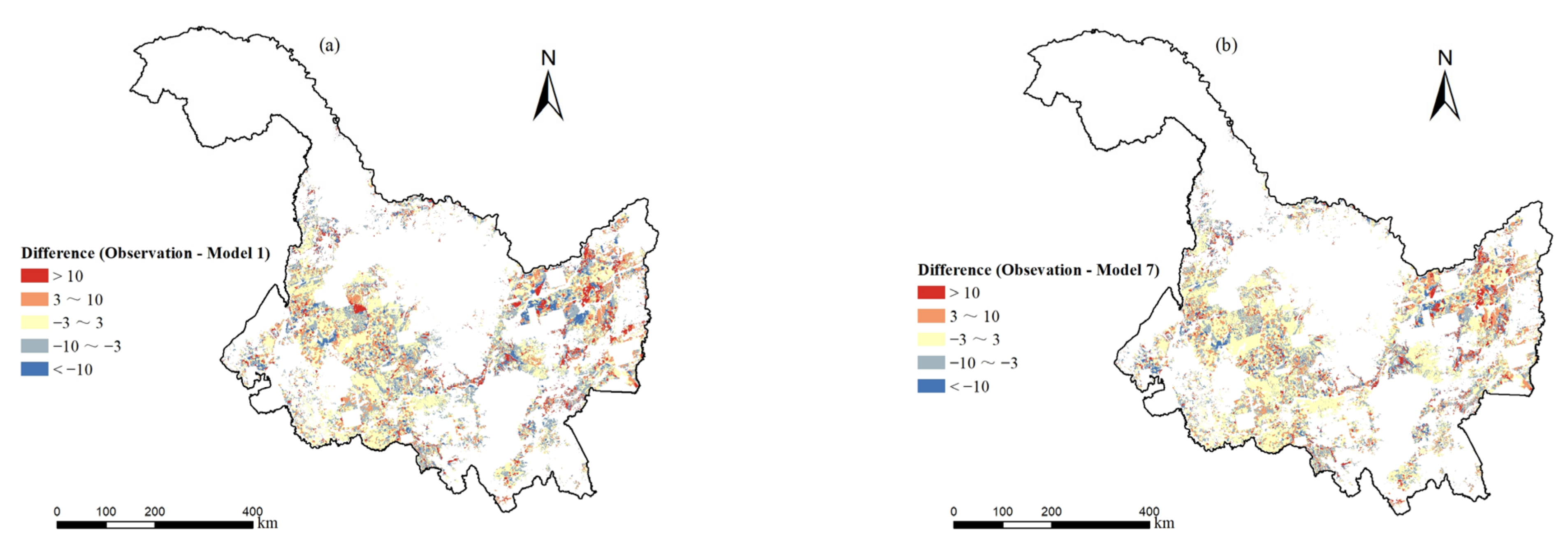
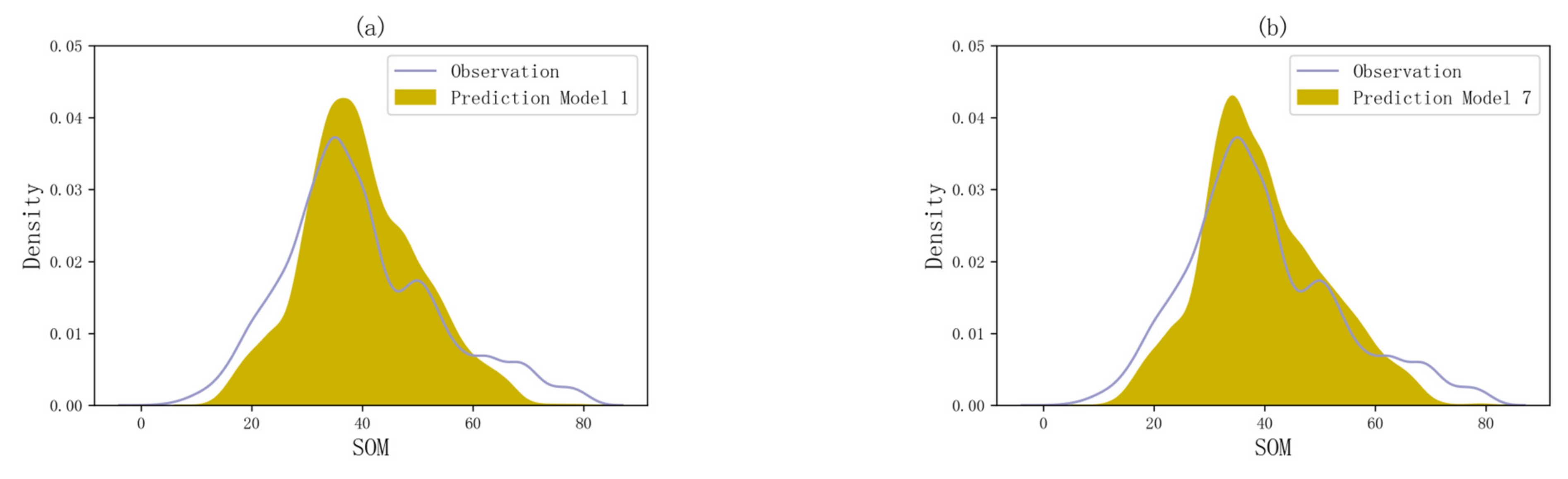
3.4. Model Performance and Spatial Difference
4. Discussion
4.1. Relative Importance of Environmental Covariates
4.2. Relative Importance of Human Activity Factors
4.3. Model Performance
4.4. Limitations and Outlook
5. Conclusions
Author Contributions
Funding
Data Availability Statement
Acknowledgments
Conflicts of Interest
References
- Qi, L.; Wang, S.; Zhuang, Q.; Yang, Z.; Bai, S.; Jin, X.; Lei, G. Spatial-temporal changes in soil organic carbon and pH in the Liaoning Province of China: A modeling analysis based on observational data. Sustainability 2019, 11, 3569. [Google Scholar] [CrossRef] [Green Version]
- Dick, W. Organic carbon, nitrogen, and phosphorus concentrations and pH in soil profiles as affected by tillage intensity. Soil Sci. Soc. Am. J. 1983, 47, 102–107. [Google Scholar] [CrossRef]
- Post, W.M.; Kwon, K.C. Soil carbon sequestration and land-use change: Processes and potential. Glob. Chang. Biol. 2000, 6, 317–327. [Google Scholar] [CrossRef] [Green Version]
- Yang, L.; Song, M.; Zhu, A.-X.; Qin, C.; Zhou, C.; Qi, F.; Li, X.; Chen, Z.; Gao, B. Predicting soil organic carbon content in croplands using crop rotation and Fourier transform decomposed variables. Geoderma 2019, 340, 289–302. [Google Scholar] [CrossRef]
- Hoffmann, M.; Pohl, M.; Jurisch, N.; Prescher, A.-K.; Campa, E.M.; Hagemann, U.; Remus, R.; Verch, G.; Sommer, M.; Augustin, J. Maize carbon dynamics are driven by soil erosion state and plant phenology rather than nitrogen fertilization form. Soil Tillage Res. 2018, 175, 255–266. [Google Scholar] [CrossRef]
- Yang, L.; He, X.; Shen, F.; Zhou, C.; Zhu, A.-X.; Gao, B.; Chen, Z.; Li, M. Improving prediction of soil organic carbon content in croplands using phenological parameters extracted from NDVI time series data. Soil Tillage Res. 2020, 196, 104465. [Google Scholar] [CrossRef]
- Wang, Y.; Wang, S.; Adhikari, K.; Wang, Q.; Sui, Y.; Xin, G. Effect of cultivation history on soil organic carbon status of arable land in northeastern China. Geoderma 2019, 342, 55–64. [Google Scholar] [CrossRef]
- Paustian, K.; Andren, O.; Janzen, H.; Lal, R.; Smith, P.; Tian, G.; Tiessen, H.; Van Noordwijk, M.; Woomer, P. Agricultural soils as a sink to mitigate CO2 emissions. Soil Use Manag. 1997, 13, 230–244. [Google Scholar] [CrossRef]
- Lal, R. Soil carbon sequestration impacts on global climate change and food security. Science 2004, 304, 1623–1627. [Google Scholar] [CrossRef] [Green Version]
- Smith, P. Carbon sequestration in croplands: The potential in Europe and the global context. Eur. J. Agron. 2004, 20, 229–236. [Google Scholar] [CrossRef]
- Hans, J. Factors of Soil Formation: A System of Quantitative Pedology; Dover Publication: Mineola, NY, USA, 1941. [Google Scholar]
- McBratney, A.B.; Santos, M.M.; Minasny, B. On digital soil mapping. Geoderma 2003, 117, 3–52. [Google Scholar] [CrossRef]
- Hamzehpour, N.; Shafizadeh-Moghadam, H.; Valavi, R. Exploring the driving forces and digital mapping of soil organic carbon using remote sensing and soil texture. Catena 2019, 182, 104141. [Google Scholar] [CrossRef]
- Ramcharan, A.; Hengl, T.; Nauman, T.; Brungard, C.; Waltman, S.; Wills, S.; Thompson, J. Soil property and class maps of the conterminous United States at 100-meter spatial resolution. Soil Sci. Soc. Am. J. 2018, 82, 186–201. [Google Scholar] [CrossRef] [Green Version]
- Hengl, T.; de Jesus, J.M.; Heuvelink, G.B.; Gonzalez, M.R.; Kilibarda, M.; Blagotić, A.; Shangguan, W.; Wright, M.N.; Geng, X.; Bauer-Marschallinger, B. SoilGrids250m: Global gridded soil information based on machine learning. PLoS ONE 2017, 12, e0169748. [Google Scholar] [CrossRef] [Green Version]
- Grunwald, S.; Thompson, J.; Boettinger, J. Digital soil mapping and modeling at continental scales: Finding solutions for global issues. Soil Sci. Soc. Am. J. 2011, 75, 1201–1213. [Google Scholar] [CrossRef]
- Liang, Z.; Chen, S.; Yang, Y.; Zhao, R.; Shi, Z.; Rossel, R.A.V. National digital soil map of organic matter in topsoil and its associated uncertainty in 1980’s China. Geoderma 2019, 335, 47–56. [Google Scholar] [CrossRef]
- Hengl, T.; Leenaars, J.G.; Shepherd, K.D.; Walsh, M.G.; Heuvelink, G.B.; Mamo, T.; Tilahun, H.; Berkhout, E.; Cooper, M.; Fegraus, E. Soil nutrient maps of Sub-Saharan Africa: Assessment of soil nutrient content at 250 m spatial resolution using machine learning. Nutr. Cycl. Agroecosyst. 2017, 109, 77–102. [Google Scholar] [CrossRef] [Green Version]
- Zhou, Y.; Hartemink, A.E.; Shi, Z.; Liang, Z.; Lu, Y. Land use and climate change effects on soil organic carbon in North and Northeast China. Sci. Total Environ. 2019, 647, 1230–1238. [Google Scholar] [CrossRef]
- Wadoux, A.M.-C. Using deep learning for multivariate mapping of soil with quantified uncertainty. Geoderma 2019, 351, 59–70. [Google Scholar] [CrossRef] [Green Version]
- Zhao, R.; Biswas, A.; Zhou, Y.; Zhou, Y.; Shi, Z.; Li, H. Identifying localized and scale-specific multivariate controls of soil organic matter variations using multiple wavelet coherence. Sci. Total Environ. 2018, 643, 548–558. [Google Scholar] [CrossRef]
- Ou, Y.; Rousseau, A.N.; Wang, L.; Yan, B. Spatio-temporal patterns of soil organic carbon and pH in relation to environmental factors—A case study of the Black Soil Region of Northeastern China. Agric. Ecosyst. Environ. 2017, 245, 22–31. [Google Scholar] [CrossRef]
- Zhang, Y.; Wu, Y.; Liu, B.; Zheng, Q.; Yin, J. Characteristics and factors controlling the development of ephemeral gullies in cultivated catchments of black soil region, Northeast China. Soil Tillage Res. 2007, 96, 28–41. [Google Scholar] [CrossRef]
- Wu, Y.; Zheng, Q.; Zhang, Y.; Liu, B.; Cheng, H.; Wang, Y. Development of gullies and sediment production in the black soil region of northeastern China. Geomorphology 2008, 101, 683–691. [Google Scholar] [CrossRef]
- Jiao, X.; Gao, C.; Sui, Y.; Lü, G.; Wei, D. Effects of long-term fertilization on soil carbon and nitrogen in Chinese Mollisols. Agron. J. 2014, 106, 1018–1024. [Google Scholar] [CrossRef]
- Chun-hua, Z.; Zong-ming, W.; Chun-ying, R.; Bai, Z.; Kai-shan, S.; Dian-wei, L. Temporal and spatial variations of soil organic and total nitrogen in the Songnen Plain maize belt. Geogr. Reserach 2011, 30, 256–268. [Google Scholar]
- Zhao, Y.; Jiang, Q.; Wang, Z. The System Evaluation of Grain Production Efficiency and Analysis of Driving Factors in Heilongjiang Province. Water 2019, 11, 1073. [Google Scholar] [CrossRef] [Green Version]
- Xu, S. Temporal and Spatial Characteristics of the Change of Cultivated Land Resources in the Black Soil Region of Heilongjiang Province (China). Sustainability 2019, 11, 38. [Google Scholar] [CrossRef] [Green Version]
- NY/T1121.6-2006; Soil Testing-Part 6: Method for Determination of Soil Organic Matter. Ministry of Agriculture: Beijing, China, 2006.
- Danielson, J.J.; Gesch, D.B. Global Multi-Resolution Terrain Elevation Data 2010 (GMTED2010); US Department of the Interior, US Geological Survey: Washington, DC, USA, 2011.
- Sayre, R.; Dangermond, J.; Frye, C.; Vaughan, R.; Aniello, P.; Breyer, S.; Cribbs, D.; Hopkins, D.; Nauman, R.; Derrenbacher, W. A New Map of Global Ecological Land Units—An Ecophysiographic Stratification Approach; Association of American Geographers: Washington, DC, USA, 2014. [Google Scholar]
- Pelletier, J.D.; Broxton, P.D.; Hazenberg, P.; Zeng, X.; Troch, P.A.; Niu, G.Y.; Williams, Z.; Brunke, M.A.; Gochis, D. A gridded global data set of soil, intact regolith, and sedimentary deposit thicknesses for regional and global land surface modeling. J. Adv. Model. Earth Syst. 2016, 8, 41–65. [Google Scholar] [CrossRef]
- Pelletier, J.; Broxton, P.; Hazenberg, P.; Zeng, X.; Troch, P.; Niu, G.; Williams, Z.; Brunke, M.; Gochis, D. Global 1-km Gridded Thickness of Soil, Regolith, and Sedimentary Deposit Layers; ORNL DAAC: Oak Ridge, TN, USA, 2016. [Google Scholar]
- Abatzoglou, J.T.; Dobrowski, S.Z.; Parks, S.A.; Hegewisch, K.C. TerraClimate, a high-resolution global dataset of monthly climate and climatic water balance from 1958–2015. Sci. Data 2018, 5, 170191. [Google Scholar] [CrossRef] [Green Version]
- Fan, Y.; Li, H.; Miguez-Macho, G. Global patterns of groundwater table depth. Science 2013, 339, 940–943. [Google Scholar] [CrossRef] [Green Version]
- Pekel, J.-F.; Cottam, A.; Gorelick, N.; Belward, A.S. High-resolution mapping of global surface water and its long-term changes. Nature 2016, 540, 418–422. [Google Scholar] [CrossRef] [PubMed]
- Venter, O.; Sanderson, E.W.; Magrach, A.; Allan, J.R.; Beher, J.; Jones, K.R.; Possingham, H.P.; Laurance, W.F.; Wood, P.; Fekete, B.M. Global terrestrial Human Footprint maps for 1993 and 2009. Sci. Data 2016, 3, 160067. [Google Scholar] [CrossRef] [PubMed] [Green Version]
- Mallick, J.; AlMesfer, M.K.; Singh, V.P.; Falqi, I.I.; Singh, C.K.; Alsubih, M.; Kahla, N.B. Evaluating the NDVI–Rainfall Relationship in Bisha Watershed, Saudi Arabia Using Non-Stationary Modeling Technique. Atmosphere 2021, 12, 593. [Google Scholar] [CrossRef]
- Mahmoudabadi, E.; Karimi, A.; Haghnia, G.H.; Sepehr, A. Digital soil mapping using remote sensing indices, terrain attributes, and vegetation features in the rangelands of northeastern Iran. Environ. Monit. Assess. 2017, 189, 500. [Google Scholar] [CrossRef]
- Lamichhane, S.; Kumar, L.; Wilson, B.J. Digital soil mapping algorithms and covariates for soil organic carbon mapping and their implications: A review. Geoderma 2019, 352, 395–413. [Google Scholar] [CrossRef]
- Kumari, N.; Srivastava, A.; Dumka, U.C.J.C. A long-term spatiotemporal analysis of vegetation greenness over the Himalayan Region using Google Earth Engine. Climate 2021, 9, 109. [Google Scholar] [CrossRef]
- Liu, H.; Yan, Y.; Zhang, X.; Qiu, Z.; Wang, N.; Yu, W. Remote sensing extraction of crop planting structure oriented to agricultural regionalizaiton. Chin. J. Agric. Resour. Reg. Plan. 2017, 38, 43–54. [Google Scholar]
- Yao, X.; Zhu, D.; Ye, S.; Yun, W.; Zhang, N.; Li, L.J.C.; Agriculture, E.i. A field survey system for land consolidation based on 3S and speech recognition technology. Comput. Electron. Agric. 2016, 127, 659–668. [Google Scholar] [CrossRef]
- Ye, S.; Song, C.; Shen, S.; Gao, P.; Cheng, C.; Cheng, F.; Wan, C.; Zhu, D. Spatial pattern of arable land-use intensity in China. Land Use Policy 2020, 99, 104845. [Google Scholar] [CrossRef]
- Wan, C.; Kuzyakov, Y.; Cheng, C.; Ye, S.; Gao, B.; Gao, P.; Ren, S.; Yun, W. A soil sampling design for arable land quality observation by using SPCOSA–CLHS hybrid approach. Land Degrad. Dev. 2021, 32, 4889–4906. [Google Scholar] [CrossRef]
- Liao, Y.; Wang, J.; Meng, B.; Li, X. Integration of GP and GA for mapping population distribution. Int. J. Geogr. Inf. Sci. 2010, 24, 47–67. [Google Scholar] [CrossRef]
- Kenett, D.Y.; Tumminello, M.; Madi, A.; Gur-Gershgoren, G.; Mantegna, R.N.; Ben-Jacob, E. Dominating clasp of the financial sector revealed by partial correlation analysis of the stock market. PLoS ONE 2010, 5, e15032. [Google Scholar] [CrossRef] [Green Version]
- Eichler, M.; Dahlhaus, R.; Sandkühler, J. Partial correlation analysis for the identification of synaptic connections. Biol. Cybern. 2003, 89, 289–302. [Google Scholar] [CrossRef]
- Peng, S.; Piao, S.; Ciais, P.; Myneni, R.B.; Chen, A.; Chevallier, F.; Dolman, A.J.; Janssens, I.A.; Penuelas, J.; Zhang, G. Asymmetric effects of daytime and night-time warming on Northern Hemisphere vegetation. Nature 2013, 501, 88–92. [Google Scholar] [CrossRef]
- Heung, B.; Bulmer, C.E.; Schmidt, M.G. Predictive soil parent material mapping at a regional-scale: A random forest approach. Geoderma 2014, 214, 141–154. [Google Scholar] [CrossRef]
- Zhi, J.; Zhang, G.; Yang, F.; Yang, R.; Liu, F.; Song, X.; Zhao, Y.; Li, D. Predicting mattic epipedons in the northeastern Qinghai-Tibetan Plateau using Random Forest. Geoderma Reg. 2017, 10, 1–10. [Google Scholar] [CrossRef]
- Breiman, L. Random forests. Mach. Learn. 2001, 45, 5–32. [Google Scholar] [CrossRef] [Green Version]
- Forkuor, G.; Hounkpatin, O.K.; Welp, G.; Thiel, M. High resolution mapping of soil properties using remote sensing variables in south-western Burkina Faso: A comparison of machine learning and multiple linear regression models. PLoS ONE 2017, 12, e0170478. [Google Scholar] [CrossRef]
- Akpa, S.I.; Odeh, I.O.; Bishop, T.F.; Hartemink, A.E.; Amapu, I.Y. Total soil organic carbon and carbon sequestration potential in Nigeria. Geoderma 2016, 271, 202–215. [Google Scholar] [CrossRef]
- Deng, X.; Chen, X.; Ma, W.; Ren, Z.; Zhang, M.; Grieneisen, M.L.; Long, W.; Ni, Z.; Zhan, Y.; Lv, X. Baseline map of organic carbon stock in farmland topsoil in East China. Agric. Ecosyst. Environ. 2018, 254, 213–223. [Google Scholar] [CrossRef]
- Jeong, G.; Oeverdieck, H.; Park, S.J.; Huwe, B.; Ließ, M. Spatial soil nutrients prediction using three supervised learning methods for assessment of land potentials in complex terrain. Catena 2017, 154, 73–84. [Google Scholar] [CrossRef]
- Behrens, T.; Schmidt, K.; Ramirez-Lopez, L.; Gallant, J.; Zhu, A.-X.; Scholten, T. Hyper-scale digital soil mapping and soil formation analysis. Geoderma 2014, 213, 578–588. [Google Scholar] [CrossRef]
- Grimm, R.; Behrens, T.; Märker, M.; Elsenbeer, H. Soil organic carbon concentrations and stocks on Barro Colorado Island—Digital soil mapping using Random Forests analysis. Geoderma 2008, 146, 102–113. [Google Scholar] [CrossRef]
- Shi, J.; Yang, L.; Zhu, A.; Qin, C.; Liang, P.; Zeng, C.; Pei, T. Machine-learning variables at different scales vs. Knowledge-based variables for mapping multiple soil properties. Soil Sci. Soc. Am. J. 2018, 82, 645–656. [Google Scholar] [CrossRef]
- Zeng, C.; Yang, L.; Zhu, A.-X.; Rossiter, D.G.; Liu, J.; Liu, J.; Qin, C.; Wang, D. Mapping soil organic matter concentration at different scales using a mixed geographically weighted regression method. Geoderma 2016, 281, 69–82. [Google Scholar] [CrossRef]
- Pedregosa, F.; Varoquaux, G.; Gramfort, A.; Michel, V.; Thirion, B.; Grisel, O.; Blondel, M.; Prettenhofer, P.; Weiss, R.; Dubourg, V. Scikit-learn: Machine learning in Python. J. Mach. Learn. Res. 2011, 12, 2825–2830. [Google Scholar]
- Sumfleth, K.; Duttmann, R. Prediction of soil property distribution in paddy soil landscapes using terrain data and satellite information as indicators. Ecol. Indic. 2008, 8, 485–501. [Google Scholar] [CrossRef]
- Adhikari, K.; Hartemink, A.E.; Minasny, B.; Kheir, R.B.; Greve, M.B.; Greve, M.H. Digital mapping of soil organic carbon contents and stocks in Denmark. PLoS ONE 2014, 9, e105519. [Google Scholar] [CrossRef]
- Yang, R.-M.; Zhang, G.-L.; Liu, F.; Lu, Y.-Y.; Yang, F.; Yang, F.; Yang, M.; Zhao, Y.-G.; Li, D.-C. Comparison of boosted regression tree and random forest models for mapping topsoil organic carbon concentration in an alpine ecosystem. Ecol. Indic. 2016, 60, 870–878. [Google Scholar] [CrossRef]
- Wiesmeier, M.; Urbanski, L.; Hobley, E.; Lang, B.; von Lützow, M.; Marin-Spiotta, E.; van Wesemael, B.; Rabot, E.; Ließ, M.; Garcia-Franco, N. Soil organic carbon storage as a key function of soils—A review of drivers and indicators at various scales. Geoderma 2019, 333, 149–162. [Google Scholar] [CrossRef]
- Schillaci, C.; Acutis, M.; Lombardo, L.; Lipani, A.; Fantappie, M.; Märker, M.; Saia, S. Spatio-temporal topsoil organic carbon mapping of a semi-arid Mediterranean region: The role of land use, soil texture, topographic indices and the influence of remote sensing data to modelling. Sci. Total Environ. 2017, 601, 821–832. [Google Scholar] [CrossRef] [PubMed]
- Ma, Y.; Minasny, B.; Wu, C. Mapping key soil properties to support agricultural production in Eastern China. Geoderma Reg. 2017, 10, 144–153. [Google Scholar] [CrossRef]
- Wang, S.; Zhuang, Q.; Wang, Q.; Jin, X.; Han, C. Mapping stocks of soil organic carbon and soil total nitrogen in Liaoning Province of China. Geoderma 2017, 305, 250–263. [Google Scholar] [CrossRef]
- Chaplot, V.; Bouahom, B.; Valentin, C. Soil organic carbon stocks in Laos: Spatial variations and controlling factors. Glob. Change Biol. 2010, 16, 1380–1393. [Google Scholar] [CrossRef]
- Doetterl, S.; Stevens, A.; Six, J.; Merckx, R.; Van Oost, K.; Pinto, M.C.; Casanova-Katny, A.; Muñoz, C.; Boudin, M.; Venegas, E.Z. Soil carbon storage controlled by interactions between geochemistry and climate. Nat. Geosci. 2015, 8, 780–783. [Google Scholar] [CrossRef]
- Meier, I.C.; Leuschner, C. Variation of soil and biomass carbon pools in beech forests across a precipitation gradient. Glob. Change Biol. 2010, 16, 1035–1045. [Google Scholar] [CrossRef]
- Conant, R.T.; Ryan, M.G.; Ågren, G.I.; Birge, H.E.; Davidson, E.A.; Eliasson, P.E.; Evans, S.E.; Frey, S.D.; Giardina, C.P.; Hopkins, F.M. Temperature and soil organic matter decomposition rates–synthesis of current knowledge and a way forward. Glob. Chang. Biol. 2011, 17, 3392–3404. [Google Scholar] [CrossRef]
- Davidson, E.A.; Janssens, I.A. Temperature sensitivity of soil carbon decomposition and feedbacks to climate change. Nature 2006, 440, 165–173. [Google Scholar] [CrossRef]
- Von Lützow, M.; Kögel-Knabner, I. Temperature sensitivity of soil organic matter decomposition—What do we know? Biol. Fertil. Soils 2009, 46, 1–15. [Google Scholar] [CrossRef]
- Stumpf, F.; Keller, A.; Schmidt, K.; Mayr, A.; Gubler, A.; Schaepman, M. Spatio-temporal land use dynamics and soil organic carbon in Swiss agroecosystems. Agric. Ecosyst. Environ. 2018, 258, 129–142. [Google Scholar] [CrossRef]
- Song, X.-D.; Yang, F.; Ju, B.; Li, D.-C.; Zhao, Y.-G.; Yang, J.-L.; Zhang, G.-L. The influence of the conversion of grassland to cropland on changes in soil organic carbon and total nitrogen stocks in the Songnen Plain of Northeast China. Catena 2018, 171, 588–601. [Google Scholar] [CrossRef]
- Peng, Y.; Xiong, X.; Adhikari, K.; Knadel, M.; Grunwald, S.; Greve, M.H. Modeling soil organic carbon at regional scale by combining multi-spectral images with laboratory spectra. PLoS ONE 2015, 10, e0142295. [Google Scholar] [CrossRef] [Green Version]
- Paul, E.A. The nature and dynamics of soil organic matter: Plant inputs, microbial transformations, and organic matter stabilization. Soil Biol. Biochem. 2016, 98, 109–126. [Google Scholar] [CrossRef] [Green Version]
- Brady, N.C.; Weil, R.R.; Weil, R.R. The Nature and Properties of Soils; Prentice Hall: Hoboken, NJ, USA, 2008; Volume 13. [Google Scholar]
- Frank, D.A.; Pontes, A.W.; McFarlane, K.J. Controls on soil organic carbon stocks and turnover among North American ecosystems. Ecosystems 2012, 15, 604–615. [Google Scholar] [CrossRef]
- Gray, J.M.; Bishop, T.F.; Wilson, B.R. Factors controlling soil organic carbon stocks with depth in eastern Australia. Soil Sci. Soc. Am. J. 2015, 79, 1741–1751. [Google Scholar] [CrossRef] [Green Version]
- Dong, W.; Wu, T.; Luo, J.; Sun, Y.; Xia, L. Land parcel-based digital soil mapping of soil nutrient properties in an alluvial-diluvia plain agricultural area in China. Geoderma 2019, 340, 234–248. [Google Scholar] [CrossRef]
- Meersmans, J.; De Ridder, F.; Canters, F.; De Baets, S.; Van Molle, M. A multiple regression approach to assess the spatial distribution of Soil Organic Carbon (SOC) at the regional scale (Flanders, Belgium). Geoderma 2008, 143, 1–13. [Google Scholar] [CrossRef]
- Tan, Z.; Lal, R.; Smeck, N.; Calhoun, F. Relationships between surface soil organic carbon pool and site variables. Geoderma 2004, 121, 187–195. [Google Scholar] [CrossRef]
- Vasques, G.; Grunwald, S.; Comerford, N.; Sickman, J. Regional modelling of soil carbon at multiple depths within a subtropical watershed. Geoderma 2010, 156, 326–336. [Google Scholar] [CrossRef]
- Russell, A.E.; Laird, D.; Parkin, T.B.; Mallarino, A.P. Impact of nitrogen fertilization and cropping system on carbon sequestration in Midwestern Mollisols. Soil Sci. Soc. Am. J. 2005, 69, 413–422. [Google Scholar] [CrossRef] [Green Version]
- Vieira, F.; Bayer, C.; Mielniczuk, J.; Zanatta, J.; Bissani, C. Long-term acidification of a Brazilian Acrisol as affected by no till cropping systems and nitrogen fertiliser. Soil Res. 2008, 46, 17–26. [Google Scholar] [CrossRef]
- Zhou, J.; Xia, F.; Liu, X.; He, Y.; Xu, J.; Brookes, P.C. Effects of nitrogen fertilizer on the acidification of two typical acid soils in South China. J. Soils Sed. 2014, 14, 415–422. [Google Scholar] [CrossRef]
- Haynes, R.J.; Naidu, R. Influence of lime, fertilizer and manure applications on soil organic matter content and soil physical conditions: A review. Nutr. Cycl. Agroecosyst. 1998, 51, 123–137. [Google Scholar] [CrossRef]
- Yang, X.; Zhang, X.; Fang, H.; Zhu, P.; Ren, J.; Wang, L. Long-term effects of fertilization on soil organic carbon changes in continuous corn of northeast China: RothC model simulations. Environ. Manag. 2003, 32, 459–465. [Google Scholar]
- Yang, X.; Zhang, X.; Deng, W.; Fang, H. Black soil degradation by rainfall erosion in Jilin, China. Land Degrad. Dev. 2003, 14, 409–420. [Google Scholar] [CrossRef]
- Liu, Z.; Yang, X.; Hubbard, K.G.; Lin, X. Maize potential yields and yield gaps in the changing climate of northeast China. Glob. Change Biol. 2012, 18, 3441–3454. [Google Scholar] [CrossRef]
- Song, C.; Wang, E.; Han, X.; Stirzaker, R. Crop production, soil carbon and nutrient balances as affected by fertilisation in a Mollisol agroecosystem. Nutr. Cycl. Agroecosyst. 2011, 89, 363–374. [Google Scholar] [CrossRef]
- Aguilera, E.; Lassaletta, L.; Gattinger, A.; Gimeno, B.S. Managing soil carbon for climate change mitigation and adaptation in Mediterranean cropping systems: A meta-analysis. Agric. Ecosyst. Environ. 2013, 168, 25–36. [Google Scholar] [CrossRef]
- Sainju, U.M.; Senwo, Z.N.; Nyakatawa, E.Z.; Tazisong, I.A.; Reddy, K.C. Soil carbon and nitrogen sequestration as affected by long-term tillage, cropping systems, and nitrogen fertilizer sources. Agric. Ecosyst. Environ. 2008, 127, 234–240. [Google Scholar] [CrossRef]
- Liu, X.; Herbert, S.; Hashemi, A.; Zhang, X.; Ding, G. Effects of agricultural management on soil organic matter and carbon transformation-a review. Plant Soil Environ. 2006, 52, 531. [Google Scholar] [CrossRef] [Green Version]
- Syswerda, S.; Corbin, A.; Mokma, D.; Kravchenko, A.; Robertson, G. Agricultural management and soil carbon storage in surface vs. deep layers. Soil Sci. Soc. Am. J. 2011, 75, 92–101. [Google Scholar] [CrossRef] [Green Version]
- Yang, J.; Zhang, S.; Li, Y.; Bu, K.; Zhang, Y.; Chang, L.; Zhang, Y. Dynamics of saline-alkali land and its ecological regionalization in western Songnen Plain, China. Chin. Geogr. Sci. 2010, 20, 159–166. [Google Scholar] [CrossRef] [Green Version]
- Wissing, L.; Kölbl, A.; Häusler, W.; Schad, P.; Cao, Z.-H.; Kögel-Knabner, I.J.S.; Research, T. Management-induced organic carbon accumulation in paddy soils: The role of organo-mineral associations. Soil Tillage Res. 2013, 126, 60–71. [Google Scholar] [CrossRef]
- Mi, W.; Wu, L.; Brookes, P.C.; Liu, Y.; Zhang, X.; Yang, X.J.S.; Research, T. Changes in soil organic carbon fractions under integrated management systems in a low-productivity paddy soil given different organic amendments and chemical fertilizers. Soil Tillage Res. 2016, 163, 64–70. [Google Scholar] [CrossRef]
- Somarathna, P.; Malone, B.; Minasny, B. Mapping soil organic carbon content over New South Wales, Australia using local regression kriging. Geoderma Reg. 2016, 7, 38–48. [Google Scholar] [CrossRef]
- Dorji, T.; Odeh, I.O.; Field, D.J.; Baillie, I.C. Digital soil mapping of soil organic carbon stocks under different land use and land cover types in montane ecosystems, Eastern Himalayas. For. Ecol. Manag. 2014, 318, 91–102. [Google Scholar] [CrossRef]
- Zhao, M.-S.; Rossiter, D.G.; Li, D.-C.; Zhao, Y.-G.; Liu, F.; Zhang, G.-L. Mapping soil organic matter in low-relief areas based on land surface diurnal temperature difference and a vegetation index. Ecol. Indic. 2014, 39, 120–133. [Google Scholar] [CrossRef]
- Gomes, L.C.; Faria, R.M.; de Souza, E.; Veloso, G.V.; Schaefer, C.E.G.; Fernandes Filho, E.I. Modelling and mapping soil organic carbon stocks in Brazil. Geoderma 2019, 340, 337–350. [Google Scholar] [CrossRef]
- Liang, Z.; Chen, S.; Yang, Y.; Zhou, Y.; Shi, Z. High-resolution three-dimensional mapping of soil organic carbon in China: Effects of SoilGrids products on national modeling. Sci. Total Environ. 2019, 685, 480–489. [Google Scholar] [CrossRef]
- Zhu, A.; Liu, F.; Li, B.; Pei, T.; Qin, C.; Liu, G.; Wang, Y.; Chen, Y.; Ma, X.; Qi, F. Differentiation of soil conditions over low relief areas using feedback dynamic patterns. Soil Sci. Soc. Am. J. 2010, 74, 861–869. [Google Scholar] [CrossRef] [Green Version]
- Zeng, C.; Zhu, A.-X.; Liu, F.; Yang, L.; Rossiter, D.G.; Liu, J.; Wang, D. The impact of rainfall magnitude on the performance of digital soil mapping over low-relief areas using a land surface dynamic feedback method. Ecol. Indic. 2017, 72, 297–309. [Google Scholar] [CrossRef]


| Forming Factors | Variables | Data Sources | Time Span |
|---|---|---|---|
| Topography | Elevation | GMTED 2010 [30] | - |
| Aspect | Processed from Elevation data | - | |
| Slope | Processed from Elevation data | - | |
| Landform class | Global Ecological Land Units [31] | 2008–2013 | |
| Climate | Annual average precipitation | Resource and Environment Data Cloud Platform | 2006–2015 |
| Annual average Temperature | Resource and Environment Data Cloud Platform | 2006–2015 | |
| Parent material | Lithological unit | Global Ecological Land Units [31] | 2008–2013 |
| Vegetation | Annual average NDVI | Resource and Environment Data Cloud Platform | 2006–2015 |
| Soil | Sedimentary deposit thickness | ORNL DAAC [32,33] | - |
| Average soil moisture | TerraClimate [34] | 2009–2017 | |
| Soil type | Resource and Environment Data Cloud Platform | 1995 | |
| Water Table Depth | [35] | - | |
| Other | Solar radiation | Global Change Research Data Publishing and Repository | 2015 |
| Surface Water occurrence | [36] | 1984–2015 | |
| Human activities | Human footprint | Socioeconomic Data and Applications Center [37] | 2009 |
| Amount of fertilizer application | - | ||
| Agronomic management level | - | ||
| Crop planting type | - | ||
| Irrigation guarantee degree | - |
| Pools | Covariates |
|---|---|
| Pool 1 | environmental variates |
| Pool 2 | environmental variates + human footprint |
| Pool 3 | environmental variates + amount of fertilizer application |
| Pool 4 | environmental variates + agronomic management level |
| Pool 5 | environmental variates + crop planting type |
| Pool 6 | environmental variates + irrigation guarantee degree |
| Pool 7 | environmental variates + human footprint, amount of fertilizer application, agronomic management level, crop planting type, irrigation guarantee degree |
| Covariates | Max | Mean | Min | SD | Covariates | Max | Mean | Min | SD |
|---|---|---|---|---|---|---|---|---|---|
| SOM (g/kg) | 80.13 | 39.46 | 2.93 | 192.75 | Annual average soil moisture | 56.11 | 18.39 | 6.90 | 59.31 |
| Aspect (°) | 359.84 | 173.08 | −1.00 | 10,414.20 | Soil type | 111.55 | 45.63 | 18.39 | 205.70 |
| Elevation (m) | 799.00 | 172.88 | 35.00 | 7917.64 | Solar radiation (MJ/m2) | 5151.92 | 4668.69 | 4391.01 | 12,035.60 |
| Slope (°) | 25.64 | 1.01 | 0.00 | 2.25 | Annual average temperature (℃) | 5.60 | 3.43 | −4.87 | 2.16 |
| Landform class | 62.95 | 46.66 | 32.91 | 6.19 | Water table depth (m) | 159.03 | 2.01 | −16.37 | 27.53 |
| Human footprint | 47.00 | 12.29 | 1.00 | 37.40 | Surface Water occurrence | 96.42 | 0.31 | 0.00 | 6.55 |
| Lithological unit | 53.38 | 46.66 | 40.67 | 5.06 | Amount of fertilizer application (t/km2) | 37.82 | 17.50 | 4.31 | 51.49 |
| Annual average NDVI | 0.95 | 0.86 | 0.18 | 0.00 | Agronomic management level | 47.28 | 46.78 | 45.36 | 0.71 |
| Annual average precipitation (mm) | 690.73 | 560.67 | 430.20 | 1836.79 | Crop planting type | 80.99 | 45.92 | 35.31 | 116.10 |
| Sedimentary deposit thickness (m) | 60.00 | 32.06 | −7.00 | 399.85 | Irrigation guarantee degree | 59.98 | 46.63 | 39.89 | 67.59 |
| No. | Covariates | MAE | RMSE | LCCC | R2 |
|---|---|---|---|---|---|
| 1 | environmental variates | 5.87 | 8.37 | 0.63 | 0.41 |
| 2 | environmental variates + human footprint | 5.79 | 8.27 | 0.64 | 0.42 |
| 3 | environmental variates + amount of fertilizer application | 5.29 | 7.72 | 0.68 | 0.53 |
| 4 | environmental variates + agronomic management level | 5.66 | 8.13 | 0.65 | 0.44 |
| 5 | environmental variates + crop planting type | 5.74 | 8.18 | 0.65 | 0.44 |
| 6 | environmental variates + irrigation guarantee degree | 5.73 | 8.20 | 0.64 | 0.43 |
| 7 | environmental variates + human footprint, amount of fertilizer application, agronomic management level, crop planting type, irrigation guarantee degree | 5.02 | 7.37 | 0.70 | 0.57 |
| Number of Samples | Min (g/kg) | Mean (g/kg) | Max (g/kg) | Variance | |
|---|---|---|---|---|---|
| Level I | 536,753 | 2.93 | 44.82 | 80.12 | 203.93 |
| Level Ⅱ | 517,441 | 5.90 | 39.94 | 80.13 | 189.80 |
| Level Ⅲ | 609,342 | 3.30 | 35.04 | 80.12 | 170.48 |
| Level Ⅳ | 353,508 | 9.00 | 38.26 | 80.13 | 139.31 |
| Areas | R2 (SOM) | Predictive Models | Reference |
|---|---|---|---|
| Brazil | 0.33 | RF | [104] |
| Eastern Himalayas | 0.36 | RF | [102] |
| Denmark | 0.42 | Cubist | [63] |
| Australia | 0.25 | SVR | [101] |
| Jiangsu, China | 0.53 | RK-REML | [103] |
| China | 0.35 | XGBoost | [105] |
| Liaoning, China | 0.63 | RF | [1] |
| Northeastern China | 0.76 | BRT | [7] |
Publisher’s Note: MDPI stays neutral with regard to jurisdictional claims in published maps and institutional affiliations. |
© 2022 by the authors. Licensee MDPI, Basel, Switzerland. This article is an open access article distributed under the terms and conditions of the Creative Commons Attribution (CC BY) license (https://creativecommons.org/licenses/by/4.0/).
Share and Cite
Ning, L.; Cheng, C.; Lu, X.; Shen, S.; Zhang, L.; Mu, S.; Song, Y. Improving the Prediction of Soil Organic Matter in Arable Land Using Human Activity Factors. Water 2022, 14, 1668. https://doi.org/10.3390/w14101668
Ning L, Cheng C, Lu X, Shen S, Zhang L, Mu S, Song Y. Improving the Prediction of Soil Organic Matter in Arable Land Using Human Activity Factors. Water. 2022; 14(10):1668. https://doi.org/10.3390/w14101668
Chicago/Turabian StyleNing, Lixin, Changxiu Cheng, Xu Lu, Shi Shen, Liang Zhang, Shaomin Mu, and Yunsheng Song. 2022. "Improving the Prediction of Soil Organic Matter in Arable Land Using Human Activity Factors" Water 14, no. 10: 1668. https://doi.org/10.3390/w14101668
APA StyleNing, L., Cheng, C., Lu, X., Shen, S., Zhang, L., Mu, S., & Song, Y. (2022). Improving the Prediction of Soil Organic Matter in Arable Land Using Human Activity Factors. Water, 14(10), 1668. https://doi.org/10.3390/w14101668