
Imputation of Ammonium Nitrogen Concentration in Groundwater Based on a Machine Learning Method


Abstract
:1. Introduction
2. Materials and Methods
2.1. Materials
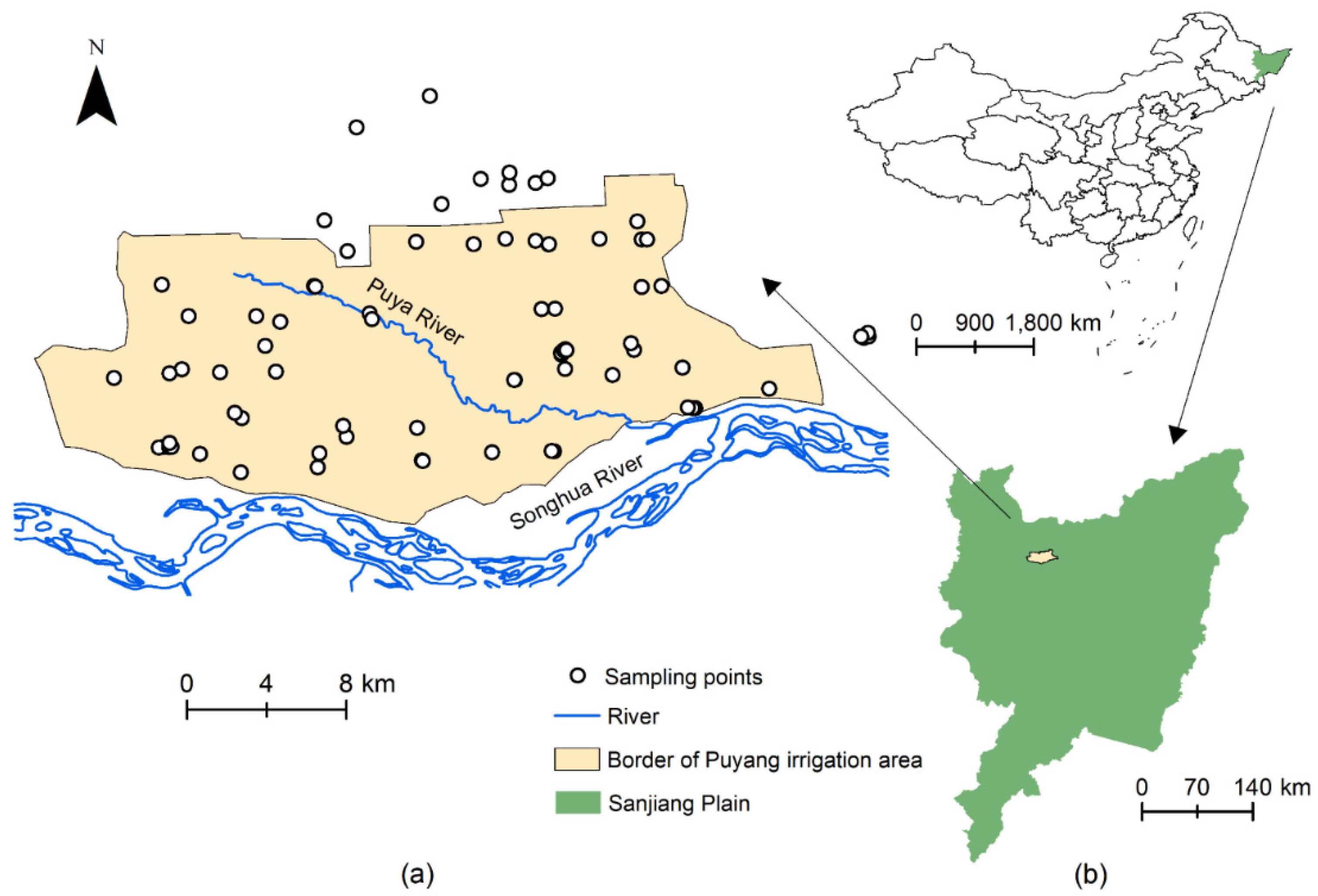
2.1.1. Study Area
2.1.2. Data
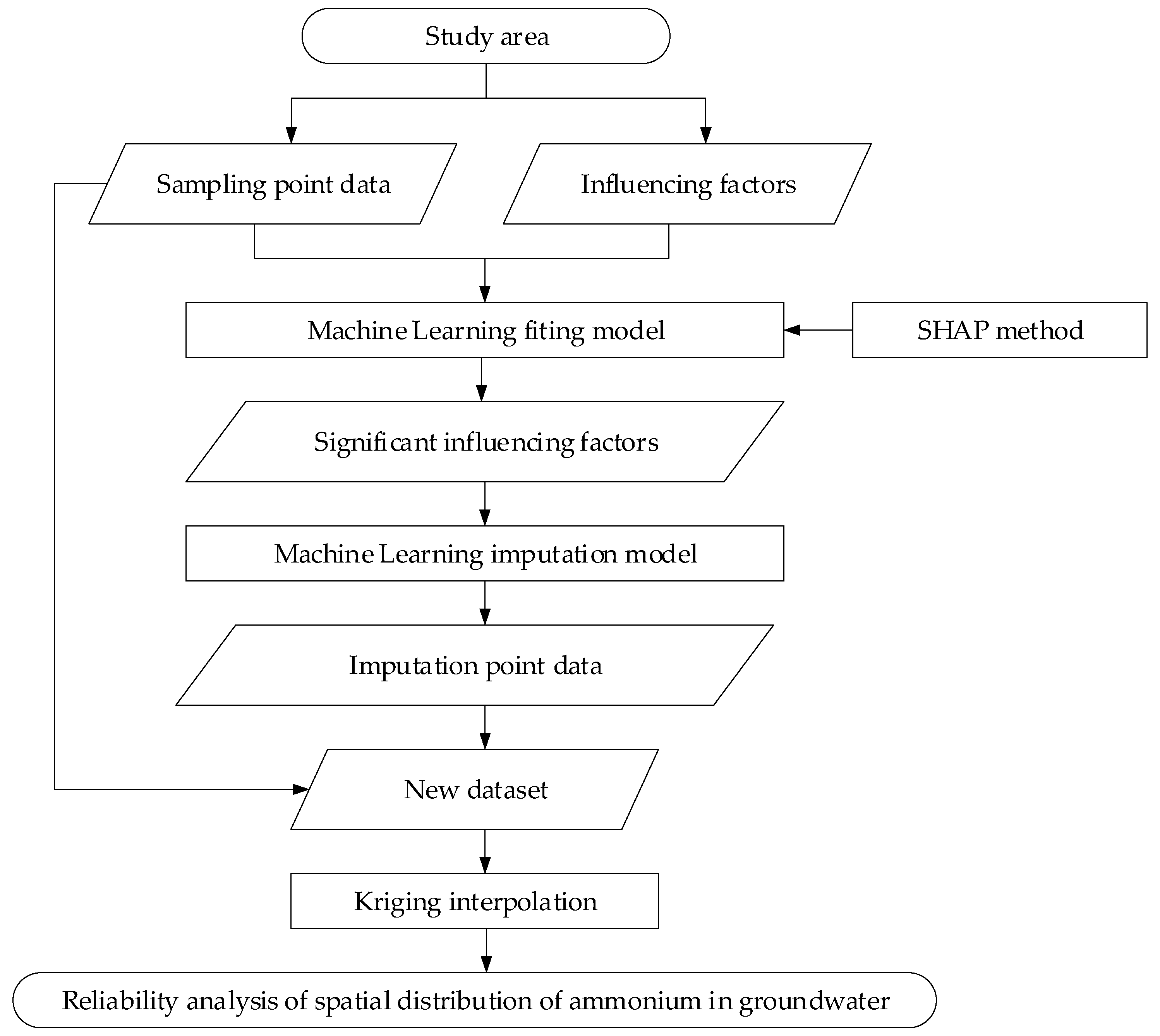
2.2. Methods
2.2.1. Random Forest Regression Model
2.2.2. Model Interpretation
2.2.3. Kriging Interpolation Method
3. Results and Discussion
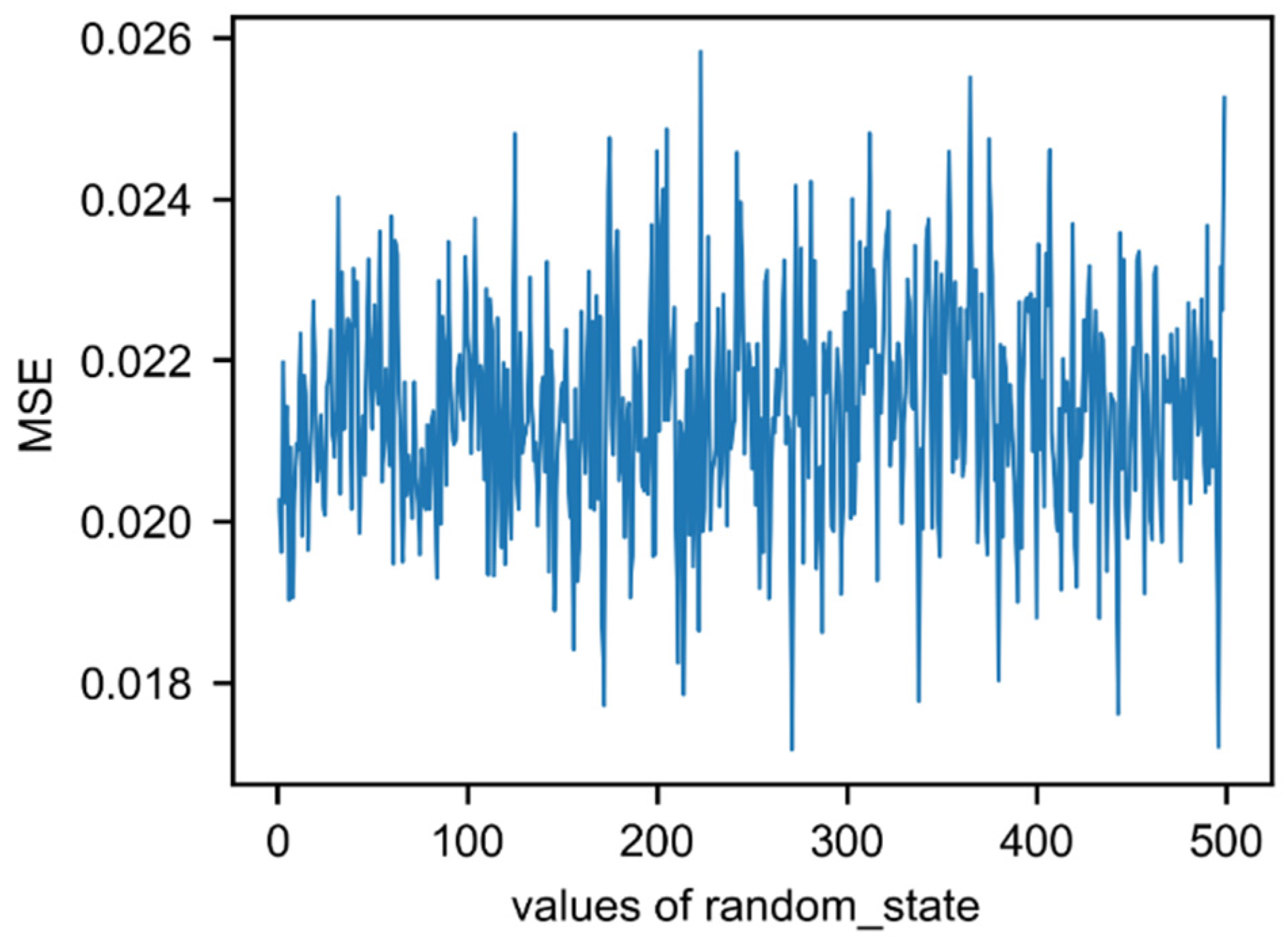
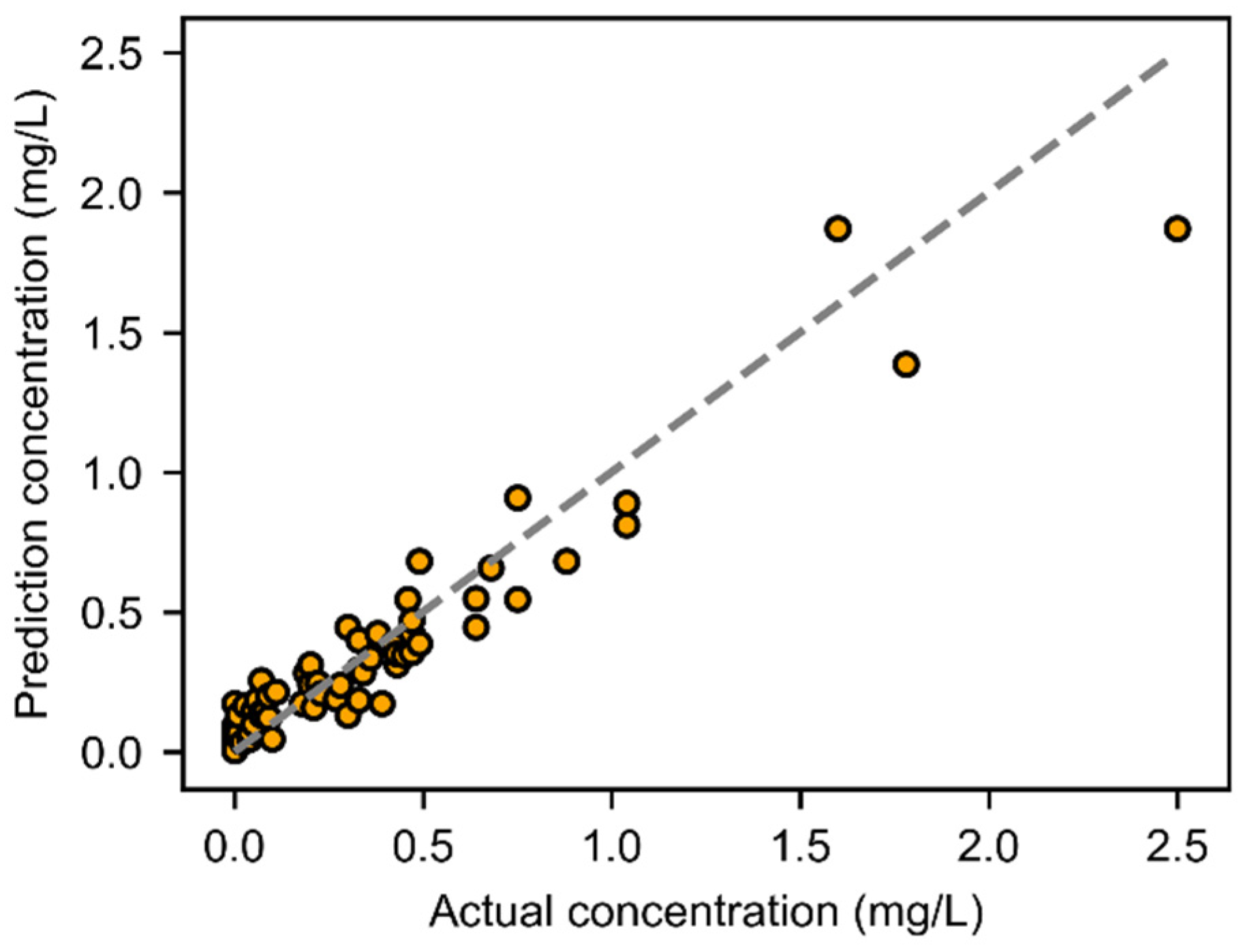
3.1. Model Performance Evaluation
3.2. Analysis the Influencing Factors of Ammonium Concentration in Groundwater
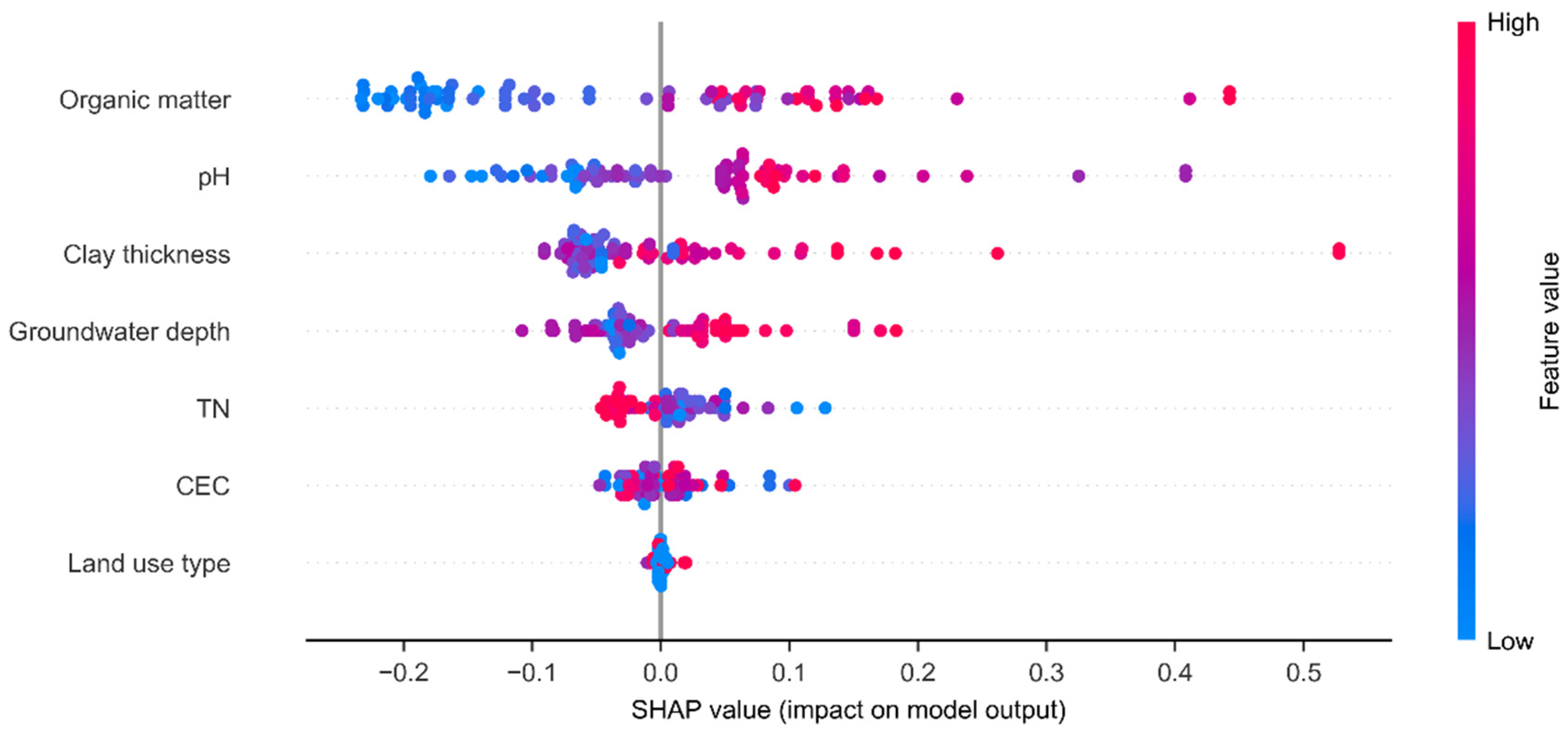
3.2.1. Feature Importance
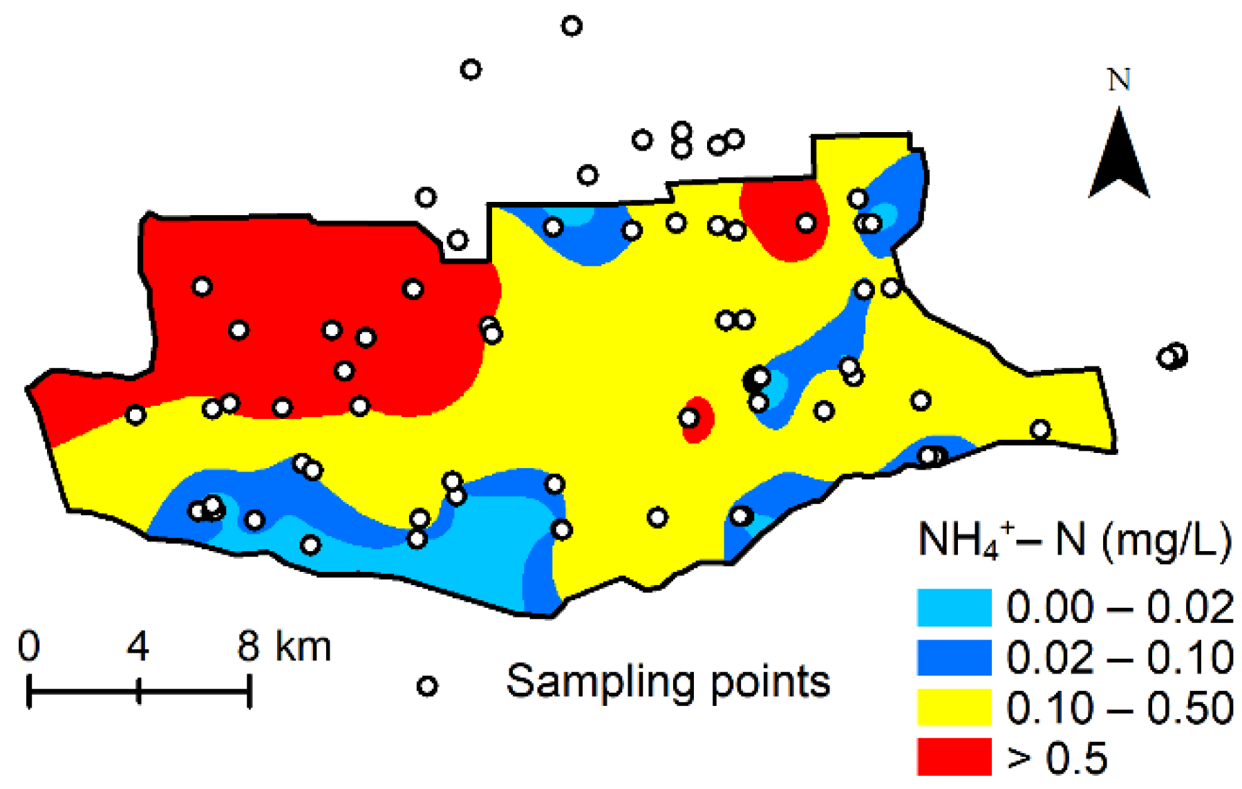
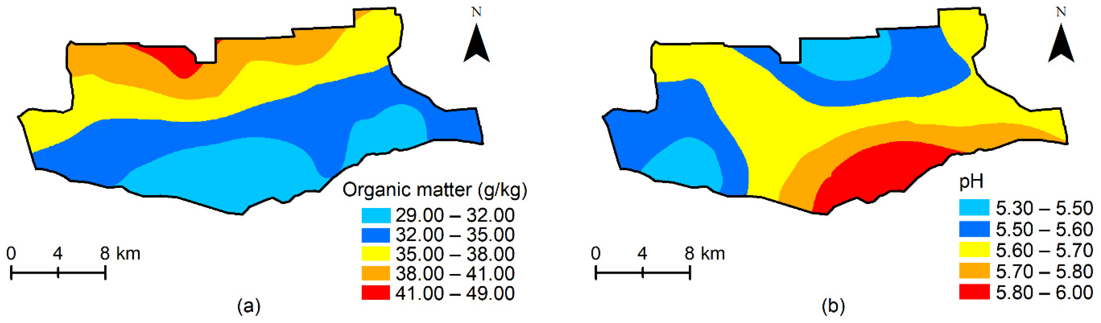
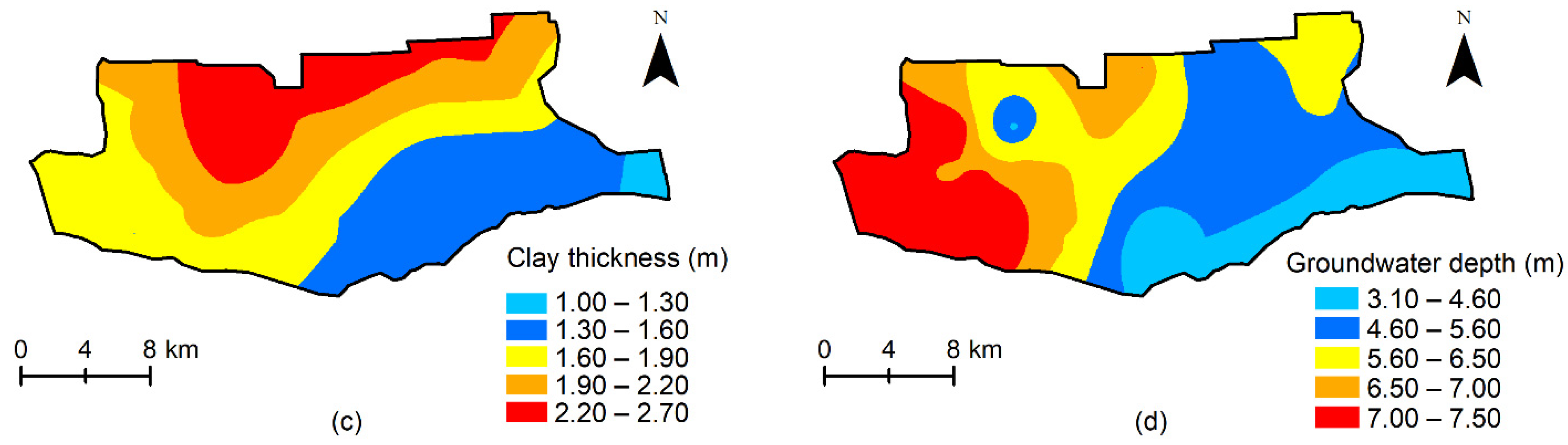
3.2.2. Spatial Distribution of the Influencing Factors
3.2.3. Feature Dependency
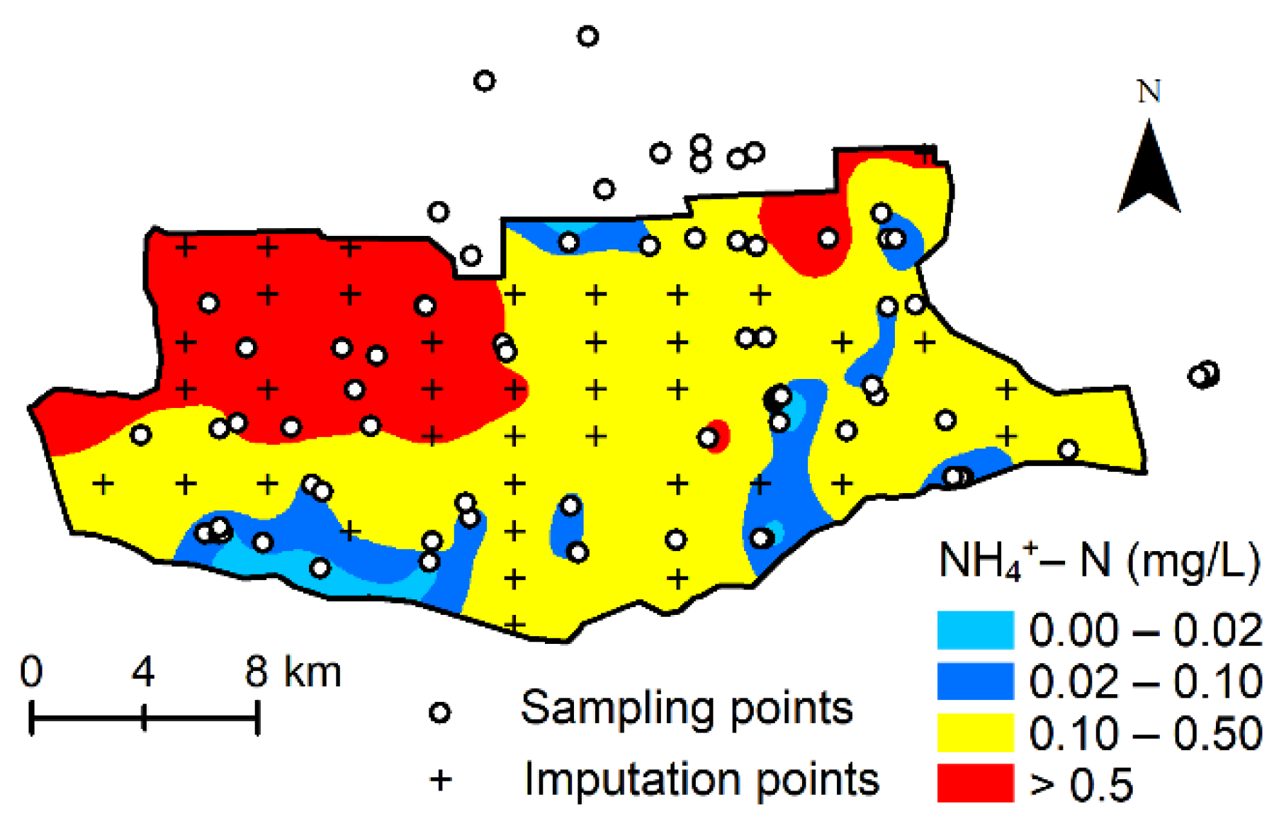
3.3. Imputation of Ammonium Concentration in Groundwater
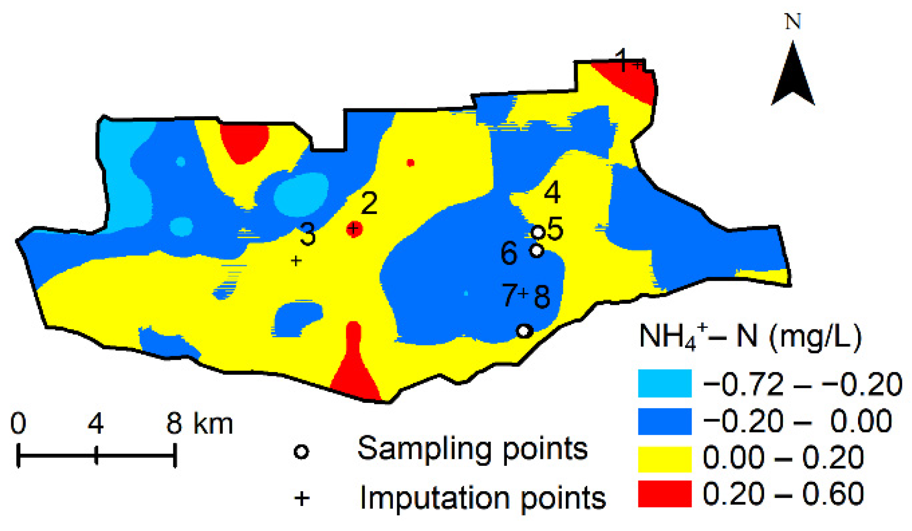
3.4. Reliability Analysis of the Results of Points Imputation Using Machine Learning Model
4. Conclusions
Author Contributions
Funding
Data Availability Statement
Conflicts of Interest
References
- Motlagh, A.M.; Yang, Z.J.; Saba, H. Groundwater quality. Water Environ. Res. 2020, 92, 1649–1658. [Google Scholar] [CrossRef]
- Shen, D.J. Groundwater management in China. Water Policy 2015, 17, 61–82. [Google Scholar] [CrossRef]
- Bierkens, M.F.P.; Wada, Y. Non-renewable groundwater use and groundwater depletion: A review. Environ. Res. Lett. 2019, 14, 063002. [Google Scholar] [CrossRef]
- Zarama-Alvarado, S. The Challenges of Dealing with Nitrogen Pollutants in Groundwater. Rev. Cient. 2018, 3, 230–242. [Google Scholar] [CrossRef]
- Norrman, J.; Sparrenbom, C.J.; Berg, M.; Nhan, D.D.; Jacks, G.; Harms-Ringdahl, P.; Nhan, P.Q.; Rosqvist, H. Tracing sources of ammonium in reducing groundwater in a well field in Hanoi (Vietnam) by means of stable nitrogen isotope (delta N-15) values. Appl. Geochem. 2015, 61, 248–258. [Google Scholar] [CrossRef]
- Su, X.; Wang, H.; Zhang, Y. Health Risk Assessment of Nitrate Contamination in Groundwater: A Case Study of an Agricultural Area in Northeast China. Water Resour. Manag. 2013, 27, 3025–3034. [Google Scholar] [CrossRef]
- Bacchus, S.T.; Barile, P.J. Discriminating sources and flowpaths of anthropogenic nitrogen discharges to Florida springs, streams and lakes. Environ. Eng. Geosci. 2005, 11, 347–369. [Google Scholar] [CrossRef] [Green Version]
- Scherger, L.E.; Zanello, V.; Lexow, C. Impact of Urea and Ammoniacal Nitrogen Wastewaters on Soil: Field Study in a Fertilizer Industry (Bahia Blanca, Argentina). Bull. Environ. Contam. Toxicol. 2021, 107, 565–573. [Google Scholar] [CrossRef]
- Lee, M.S.; Lee, K.K.; Hyun, Y.J.; Clement, T.P.; Hamilton, D. Nitrogen transformation and transport modeling in groundwater aquifers. Ecol. Model. 2006, 192, 143–159. [Google Scholar] [CrossRef] [Green Version]
- Shi, W.M.; Yao, J.; Yan, F. Vegetable cultivation under greenhouse conditions leads to rapid accumulation of nutrients, acidification and salinity of soils and groundwater contamination in South-Eastern China. Nutr. Cycl. Agroecosyst. 2009, 83, 73–84. [Google Scholar] [CrossRef]
- Li, J.; Heap, A.D. Spatial interpolation methods applied in the environmental sciences: A review. Environ. Model. Softw. 2014, 53, 173–189. [Google Scholar] [CrossRef]
- Shi, T.D.; Zhong, D.Y.; Wang, L.G. Geological Modeling Method Based on the Normal Dynamic Estimation of Sparse Point Clouds. Mathematics 2021, 9, 1819. [Google Scholar] [CrossRef]
- Zhao, Y.C.; Xu, X.H.; Tian, K.; Huang, B.A.; Hai, N. Comparison of sampling schemes for the spatial prediction of soil organic matter in a typical black soil region in China. Environ. Earth Sci. 2016, 75, 4. [Google Scholar] [CrossRef]
- Du, Y.; Deng, Y.; Ma, T.; Shen, S.; Lu, Z.; Gan, Y. Spatial Variability of Nitrate and Ammonium in Pleistocene Aquifer of Central Yangtze River Basin. Groundwater 2020, 58, 110–118. [Google Scholar] [CrossRef]
- Wang, M.X.; Liu, G.D.; Wu, W.L.; Bao, Y.H.; Liu, W.N. Prediction of agriculture derived groundwater nitrate distribution in North China Plain with GIS-based BPNN. Environ. Geol. 2006, 50, 637–644. [Google Scholar] [CrossRef]
- Liu, C.W.; Wang, Y.B.; Jang, C.S. Probability-based nitrate contamination map of groundwater in Kinmen. Environ. Monit. Assess. 2013, 185, 10147–10156. [Google Scholar] [CrossRef]
- Knoll, L.; Breuer, L.; Bach, M. Large scale prediction of groundwater nitrate concentrations from spatial data using machine learning. Sci. Total Environ. 2019, 668, 1317–1327. [Google Scholar] [CrossRef]
- Ransom, K.M.; Nolan, B.T.; Traum, J.A.; Faunt, C.C.; Bell, A.M.; Gronberg, J.A.M.; Wheeler, D.C.; Rosecrans, C.Z.; Jurgens, B.; Schwarz, G.E.; et al. A hybrid machine learning model to predict and visualize nitrate concentration throughout the Central Valley aquifer, California, USA. Sci. Total Environ. 2017, 601, 1160–1172. [Google Scholar] [CrossRef]
- Mi, J.X.; Li, A.D.; Zhou, L.F. Review Study of Interpretation Methods for Future Interpretable Machine Learning. IEEE Access 2020, 8, 191969–191985. [Google Scholar] [CrossRef]
- Althoff, D.; Bazame, H.C.; Nascimento, J.G. Untangling hybrid hydrological models with explainable artificial intelligence. H2Open J. 2021, 4, 13–28. [Google Scholar] [CrossRef]
- Thrun, M.C.; Ultsch, A.; Breuer, L. Explainable AI Framework for Multivariate Hydrochemical Time Series. Mach. Learn. Knowl. Extr. 2021, 3, 170–204. [Google Scholar] [CrossRef]
- Loh, W.-Y. Classification and regression trees. Wiley Interdiscip. Rev.-Data Min. Knowl. Discov. 2011, 1, 14–23. [Google Scholar] [CrossRef]
- Talekar, B.; Agrawal, S. A Detailed Review on Decision Tree and Random Forest. Biosci. Biotechnol. Res. Commun. 2020, 13, 245–248. [Google Scholar] [CrossRef]
- Ture, M.; Tokatli, F.; Kurt, I. Using Kaplan-Meier analysis together with decision tree methods (C&RT, CHAID, QUEST, C4.5 and ID3) in determining recurrence-free survival of breast cancer patients. Expert Syst. Appl. 2009, 36, 2017–2026. [Google Scholar] [CrossRef]
- Alves, L.G.A.; Ribeiro, H.V.; Rodrigues, F.A. Crime prediction through urban metrics and statistical learning. Phys. A-Stat. Mech. Appl. 2018, 505, 435–443. [Google Scholar] [CrossRef] [Green Version]
- Wang, Z.L.; Lai, C.G.; Chen, X.H.; Yang, B.; Zhao, S.W.; Bai, X.Y. Flood hazard risk assessment model based on random forest. J. Hydrol. 2015, 527, 1130–1141. [Google Scholar] [CrossRef]
- Tang, Z.P.; Mei, Z.; Liu, W.D.; Xia, Y. Identification of the key factors affecting Chinese carbon intensity and their historical trends using random forest algorithm. J. Geogr. Sci. 2020, 30, 743–756. [Google Scholar] [CrossRef]
- le Maire, G.; Marsden, C.; Nouvellon, Y.; Grinand, C.; Hakamada, R.; Stape, J.L.; Laclau, J.P. MODIS NDVI time-series allow the monitoring of Eucalyptus plantation biomass. Remote Sens. Environ. 2011, 115, 2613–2625. [Google Scholar] [CrossRef]
- Shin, K. Quantitative Precipitation Estimates Using Machine Learning Approaches with Operational Dual-Polarization Radar Data. Remote Sens. 2021, 13, 694. [Google Scholar] [CrossRef]
- Politikos, D.V.; Petasis, G.; Katselis, G. Interpretable machine learning to forecast hypoxia in a lagoon. Ecol. Inform. 2021, 66, 101480. [Google Scholar] [CrossRef]
- Wang, R.Z.; Kim, J.H.; Li, M.H. Predicting stream water quality under different urban development pattern scenarios with an interpretable machine learning approach. Sci. Total Environ. 2021, 761, 144057. [Google Scholar] [CrossRef]
- Parsa, A.B.; Movahedi, A.; Taghipour, H.; Derrible, S.; Mohammadian, A. Toward safer highways, application of XGBoost and SHAP for real-time accident detection and feature analysis. Accid. Anal. Prev. 2020, 136, 105405. [Google Scholar] [CrossRef]
- Lundberg, S.M.; Lee, S.-I. A Unified Approach to Interpreting Model Predictions. In Proceedings of the 31st Annual Conference on Neural Information Processing Systems (NIPS), Long Beach, CA, USA, 4–9 December 2017. [Google Scholar]
- Lundberg, S.M.; Erion, G.; Chen, H.; Degrave, A.; Prutkin, J.M.; Nair, B.; Katz, R.; Himmelfarb, J.; Bansal, N.; Lee, S.-I. From local explanations to global understanding with explainable AI for trees. Nat. Mach. Intell. 2020, 2, 56–67. [Google Scholar] [CrossRef]
- Fujimoto, K.; Kojadinovic, I.K.; Marichal, J.L. Axiomatic characterizations of probabilistic and cardinal-probabilistic interaction indices. Games Econ. Behav. 2006, 55, 72–99. [Google Scholar] [CrossRef] [Green Version]
- Negreiros, J.; Painho, M.; Aguilar, F.; Aguilar, M. Geographical Information Systems Principles of Ordinary Kriging Interpolator. J. Appl. Sci. 2010, 10, 852–867. [Google Scholar] [CrossRef] [Green Version]
- Leiv, R.G.; Fernandez Anta, A.; Mancus, V.; Casari, P. A Novel Hyperparameter-Free Approach to Decision Tree Construction That Avoids Overfitting by Design. IEEE Access 2019, 7, 99978–99987. [Google Scholar] [CrossRef]
- Bui, D.T.; Khosravi, K.; Karimi, M.; Busico, G.; Khozani, Z.S.; Nguyen, H.; Mastrocicco, M.; Tedesco, D.; Cuoco, E.; Kazakis, N. Enhancing nitrate and strontium concentration prediction in groundwater by using new data mining algorithm. Sci. Total Environ. 2020, 715, 136836. [Google Scholar] [CrossRef]
- Shen, S.; Ma, T.; Du, Y.; Luo, K.W.; Deng, Y.M.; Lu, Z.J. Temporal variations in groundwater nitrogen under intensive groundwater/surface-water interaction. Hydrogeol. J. 2019, 27, 1753–1766. [Google Scholar] [CrossRef]
- Lupon, A.; Denfeld, B.A.; Laudon, H.; Leach, J.; Sponseller, R.A. Discrete groundwater inflows influence patterns of nitrogen uptake in a boreal headwater stream. Freshw. Sci. 2020, 39, 228–240. [Google Scholar] [CrossRef] [Green Version]
- Wang, L.S.; He, Z.B.; Li, J. Assessing the land use type and environment factors affecting groundwater nitrogen in an arid oasis in northwestern China. Environ. Sci. Pollut. Res. 2020, 27, 40061–40074. [Google Scholar] [CrossRef]
- Zhao, S.; Zhang, B.J.; Zhou, N.Q. Effects of Redox Potential on the Environmental Behavior of Nitrogen in Riparian Zones of West Dongting Lake Wetlands, China. Wetlands 2020, 40, 1307–1316. [Google Scholar] [CrossRef]
- Li, D.; Zhou, Y.; Long, Q.; Li, R.; Lu, C. Ammonia nitrogen adsorption by different aquifer media: An experimental trial for nitrogen removal from groundwater. Hum. Ecol. Risk Assess. 2020, 26, 2434–2446. [Google Scholar] [CrossRef]
- Wang, C.; Wu, D.; Mao, X.; Hou, J.; Wang, L.; Han, Y. Estimating soil ammonium adsorption using pedotransfer functions in an irrigation district of the North China Plain. Pedosphere 2021, 31, 157–171. [Google Scholar] [CrossRef]
- Wang, S.; Tang, C.; Song, X.; Yuan, R.; Wang, Q.; Zhang, Y. Using major ions and delta δ15N-NO3− to identify nitrate sources and fate in an alluvial aquifer of the Baiyangdian lake watershed, North China Plain. Environ. Sci.-Processes Impacts 2013, 15, 1430–1443. [Google Scholar] [CrossRef]
- Dong, Y.B.; Lin, H. Ammonia nitrogen removal from aqueous solution using zeolite modified by microwave-sodium acetate. J. Cent. South Univ. 2016, 23, 1345–1352. [Google Scholar] [CrossRef]
- Almasri, M.N.; Kaluarachchi, J.J. Assessment and management of long-term nitrate pollution of ground water in agriculture-dominated watersheds. J. Hydrol. 2004, 295, 225–245. [Google Scholar] [CrossRef]
- Rudzianskaite, A.; Sukys, P. Effects of groundwater level fluctuation on its chemical composition in karst soils of Lithuania. Environ. Geol. 2008, 56, 289–297. [Google Scholar] [CrossRef]
- Huang, J.; Xu, J.; Liu, X.; Liu, J.; Ramsankaran, R.; Wang, L.; Su, W. Geospatial Based Assessment of Spatial Variation of Groundwater Nitrate Nitrogen in Shandong Intensive Farming Regions of China. Sens. Lett. 2012, 10, 491–500. [Google Scholar] [CrossRef]


| Factor | Description | Source | Point Number | Date | Resolution | Rmse | Place |
|---|---|---|---|---|---|---|---|
| Organic matter | Data from the special study on soil environmental quality | Kriging interpolation | 457 | October 2018 | 690 m | 16.61 | Songhua River-Naoli River Basin in Sanjiang Plain and surrounding areas |
| TN | Kriging interpolation | 457 | October 2018 | 690 m | 0.70 | ||
| CEC | Kriging interpolation | 457 | October 2018 | 690 m | 7.27 | ||
| pH | Kriging interpolation | 457 | October 2018 | 690 m | 0.49 | ||
| Groundwater depth | Groundwater sampling point data | Kriging interpolation | 275 | August 2017 | 690 m | 3.94 | |
| Clay thickness | Historical data | Kriging interpolation | 1614 | 690 m | 2.64 | ||
| Land use | Data on the relevant website | Resource and Environment Science and Data Center | 2018 | 1000 m |
| Model | Parameter | Parameter Value | MSE |
|---|---|---|---|
| Fitting model | random_state | 271 | 0.017 |
| Prediction model | max_depth | 60 | Training data MSE = 0.02 Test data MSE = 0.09 |
| n_estimators | 7 | ||
| min_impurity_decrease | 0 |
| Influencing Factor | Organic Matter | pH | Clay Thickness | Groundwater Depth |
|---|---|---|---|---|
| VIF | 3.19 | 2.07 | 3.30 | 2.01 |
| Organic Matter | pH | Clay Thickness | Groundwater Depth |
|---|---|---|---|
| 1247.91 | 31.93 | 3.08 | 31.61 |
| Point Number | Groundwater Depth (m) | Clay Thickness (m) | Organic Matter (g/kg) | pH |
|---|---|---|---|---|
| 1 | 5.71 | 2.41 | 36.00 | 5.70 |
| 2 | 4.79 | 2.11 | 36.86 | 5.63 |
| 3 | 7.04 | 2.26 | 32.92 | 5.72 |
| 4 | 4.92 | 1.37 | 32.95 | 5.63 |
| 5 | 5.03 | 1.37 | 33.13 | 5.70 |
| 6 | 4.40 | 1.37 | 31.46 | 5.85 |
| 7 | 4.35 | 1.35 | 32.27 | 5.97 |
| 8 | 4.36 | 1.35 | 32.41 | 5.98 |
Publisher’s Note: MDPI stays neutral with regard to jurisdictional claims in published maps and institutional affiliations. |
© 2022 by the authors. Licensee MDPI, Basel, Switzerland. This article is an open access article distributed under the terms and conditions of the Creative Commons Attribution (CC BY) license (https://creativecommons.org/licenses/by/4.0/).
Share and Cite
Li, W.; Ye, X.; Du, X. Imputation of Ammonium Nitrogen Concentration in Groundwater Based on a Machine Learning Method. Water 2022, 14, 1595. https://doi.org/10.3390/w14101595
Li W, Ye X, Du X. Imputation of Ammonium Nitrogen Concentration in Groundwater Based on a Machine Learning Method. Water. 2022; 14(10):1595. https://doi.org/10.3390/w14101595
Chicago/Turabian StyleLi, Wanlu, Xueyan Ye, and Xinqiang Du. 2022. "Imputation of Ammonium Nitrogen Concentration in Groundwater Based on a Machine Learning Method" Water 14, no. 10: 1595. https://doi.org/10.3390/w14101595
APA StyleLi, W., Ye, X., & Du, X. (2022). Imputation of Ammonium Nitrogen Concentration in Groundwater Based on a Machine Learning Method. Water, 14(10), 1595. https://doi.org/10.3390/w14101595