
Estimation of Scour Propagation Rates around Pipelines While Considering Simultaneous Effects of Waves and Currents Conditions


Abstract
:1. Introduction
2. Overview of Databases
2.1. Dimensional Analysis
2.2. Experimental Case
3. Strategy on Selection of Effective Parameters
4. Implementation of Soft Computing Models
4.1. Gene-Expression Programming
4.2. Multivariate Adaptive Regression Splines
4.3. M5 Model Tree
4.4. Evolutionary Polynomial Regression
5. Results and Discussion
5.1. Definition of Statistical Indices
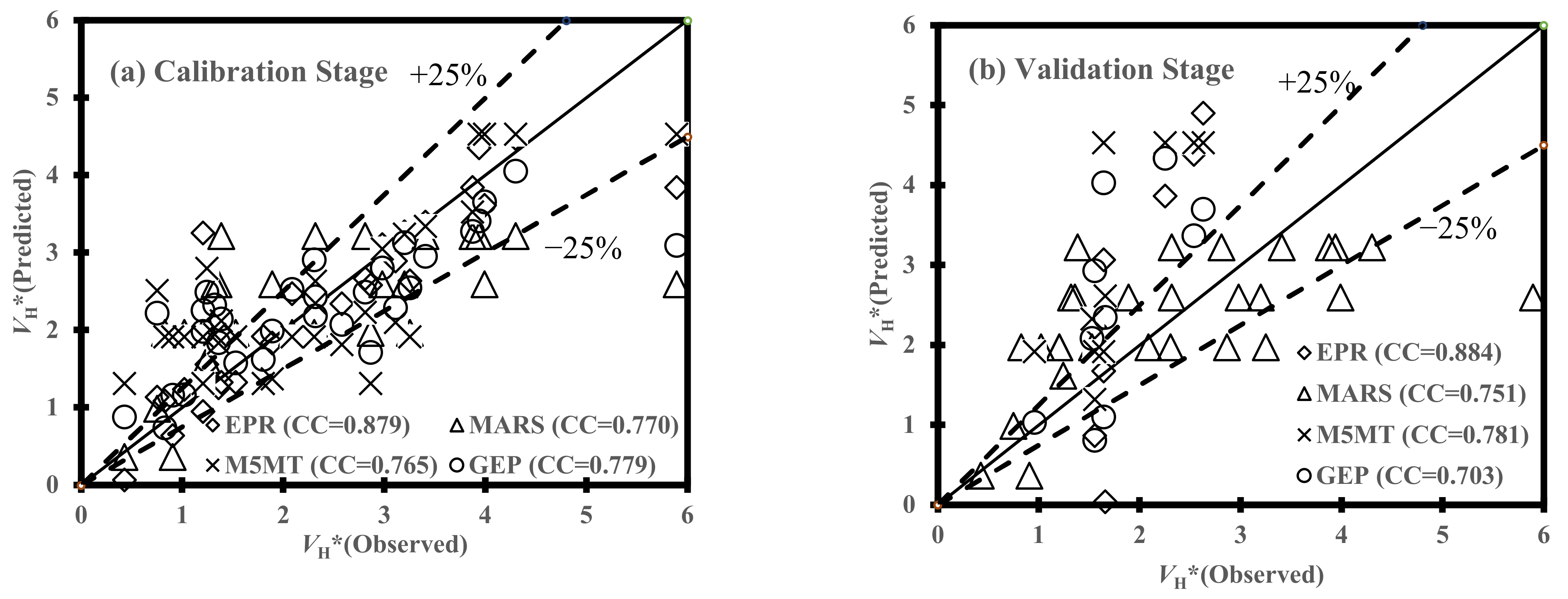
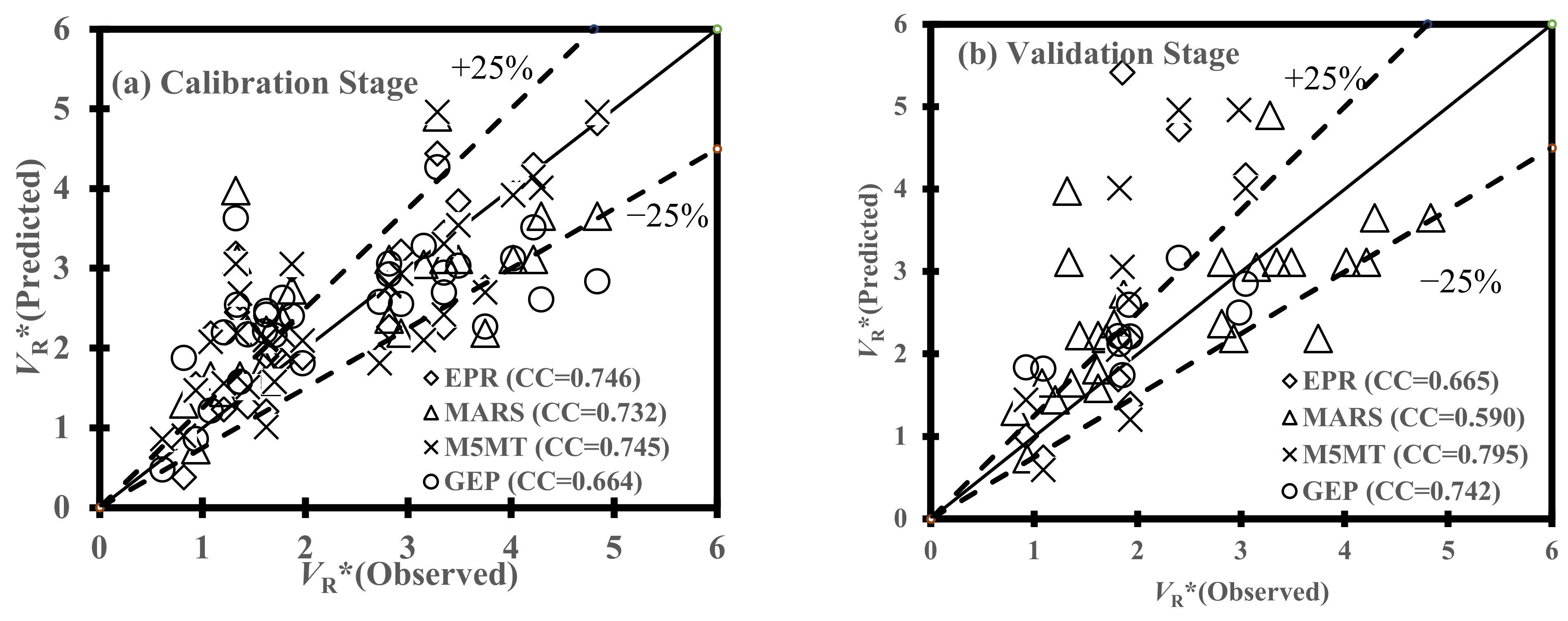
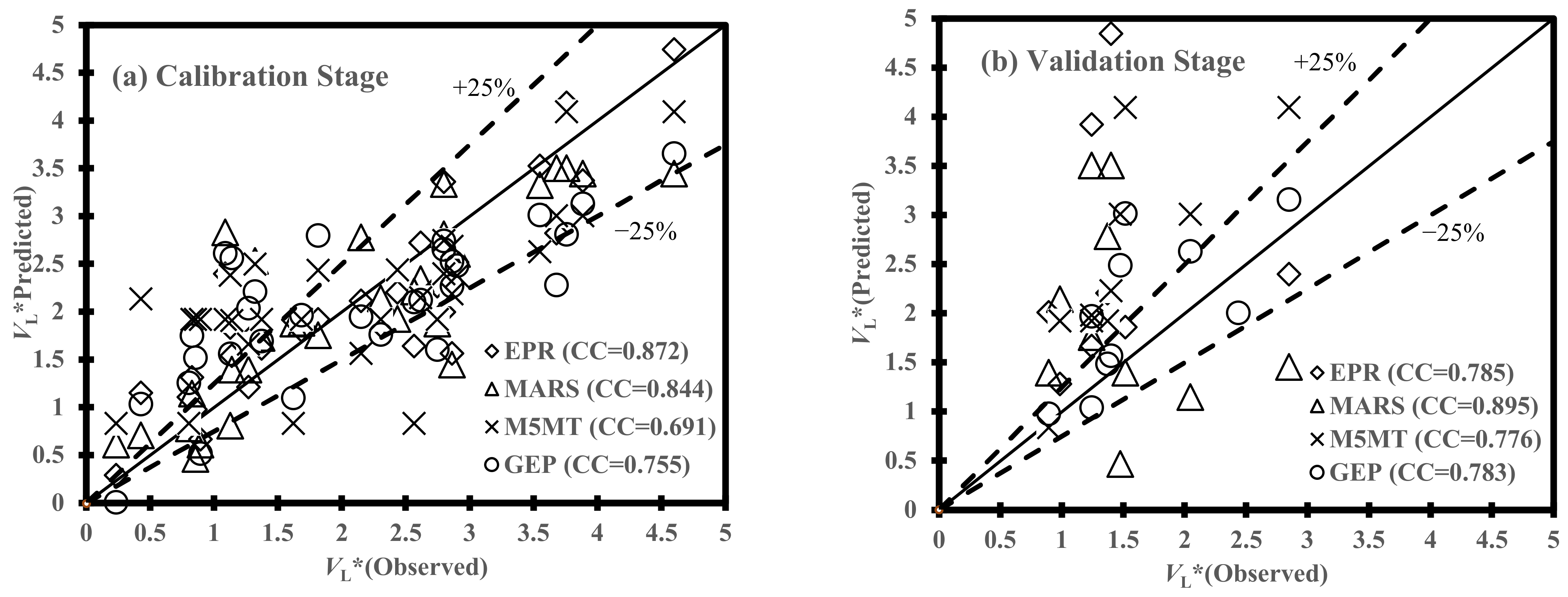
5.2. Statistical Performance of Soft Computing Techniques
5.3. Complexity of Soft Computing Techniques Performance
6. Effects of Velocity Ratio on the Scour Propagation Rates
7. Conclusions
- -
- The developments of new equations by seven combinations of dimensionless parameters showed that the present predictive techniques raised three chief merits: (i) providing mathematical expressions by EPR and GEP with complicated terms (as naturally found in the scour propagation around offshore pipelines) when fed by a limited number of scouring tests, (ii) on the contrary, equations by M5MT and MARS models reduced the complexity of the evaluation of scouring process by providing simpler regression equations, and (iii) selecting optimal combination of the effective dimensionless parameters (from θC, θW, e/D, KC, and m) played a key role in the prediction of the scour propagation rates;
- -
- From the calibration and validation phases, the performance of AI models indicated a reasonable degree of efficiency for the estimation of the scour propagation rates. More specifically, statistical measures demonstrated that Equations (20) and (21) given by the GEP model had the best performance in the estimation of VR* and VH*, respectively, whereas the MARS model [Equation (25)] indicated the most accurate efficiency for the evaluation of VL*. On the other hand, the sixth combination of effective parameters (i.e., m θC,(1 − m)θW, 1 − e/D, KC) provided the best results for the scour propagation rates in the right and left hands of pipelines (VR* and VL*) when the GEP and MARS models fed, respectively. In the case of VH*, the MARS model fed by the fifth combination of dimensionless parameters (i.e., F, θC, θW,m,e/D) demonstrated the best performance. Generally, it was inferred that the performance of AI models stood at the highest level of accuracy when θC, θW, and m were not converted to one dimensionless parameter [mθC + (1 − m)θW].
- -
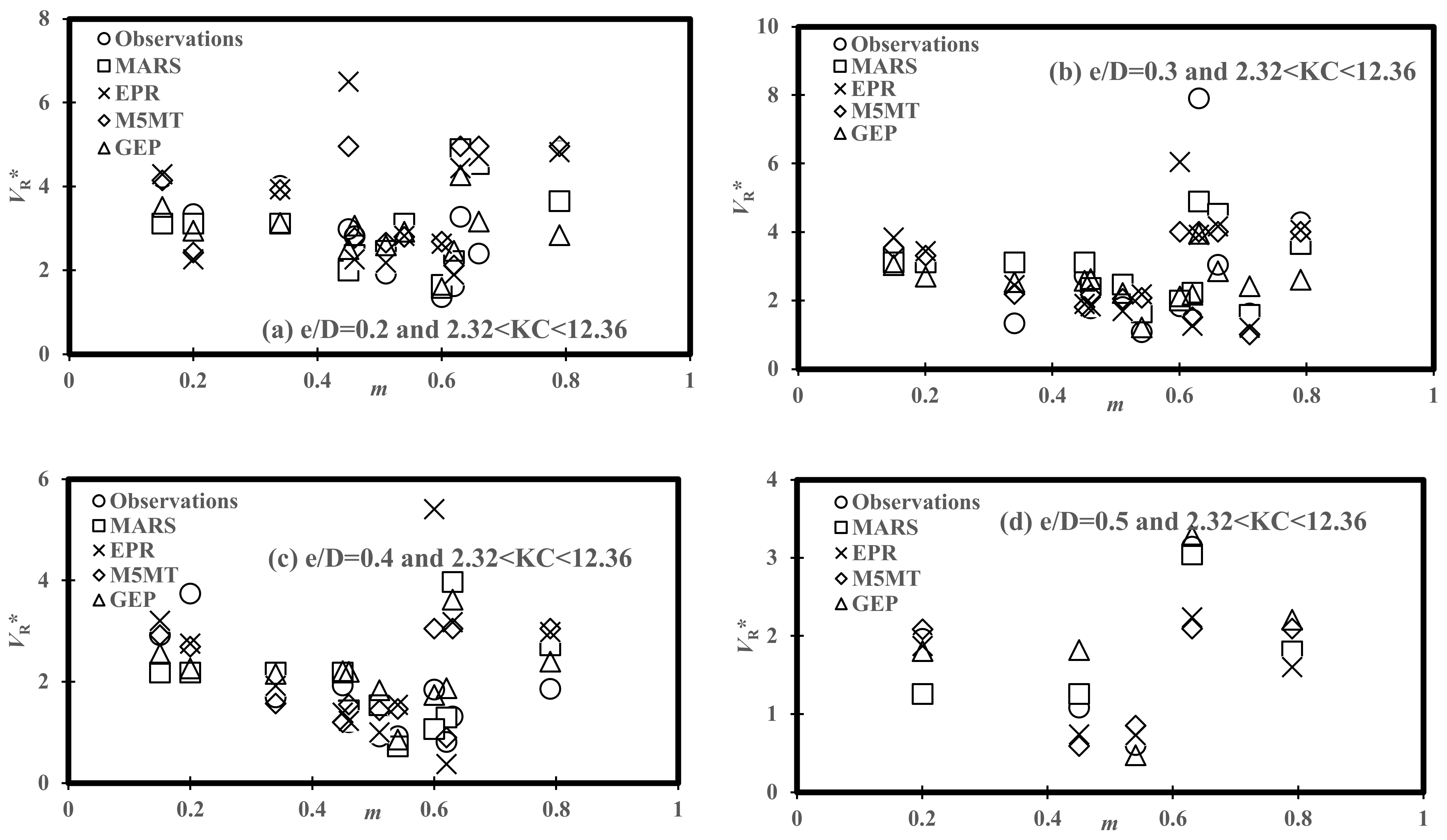
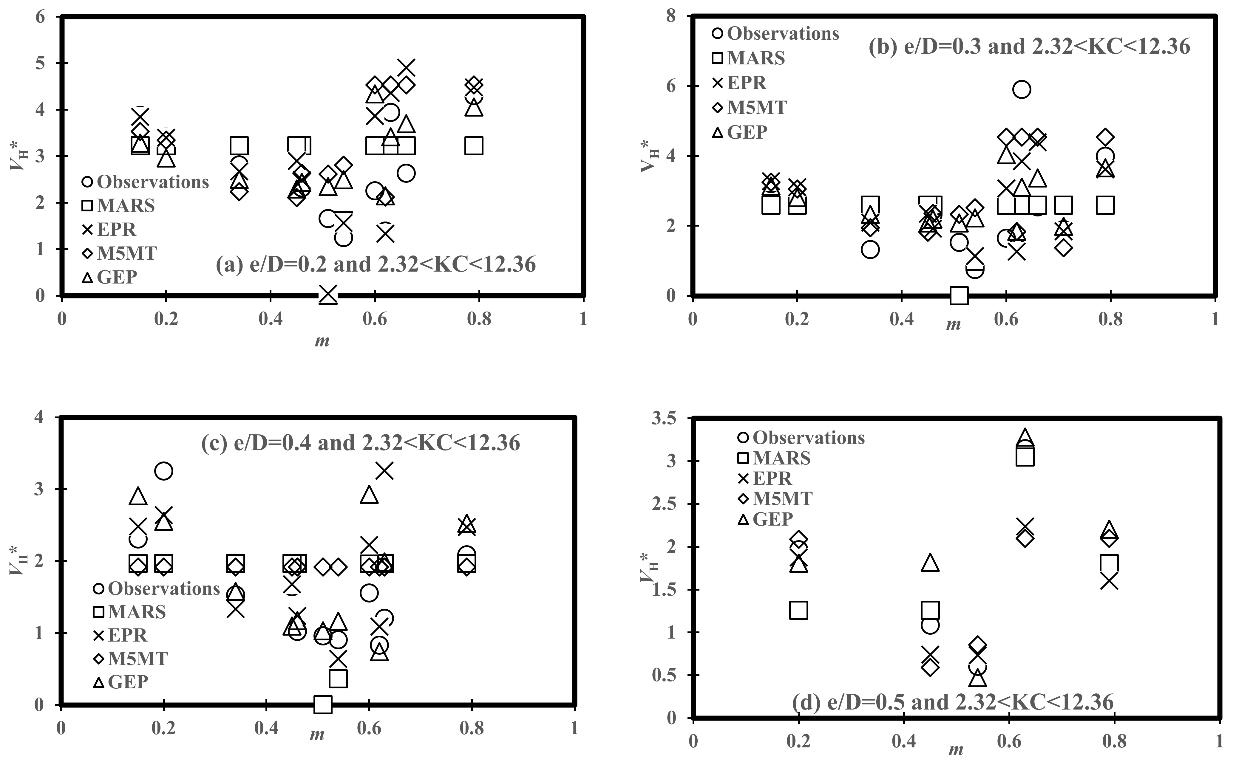
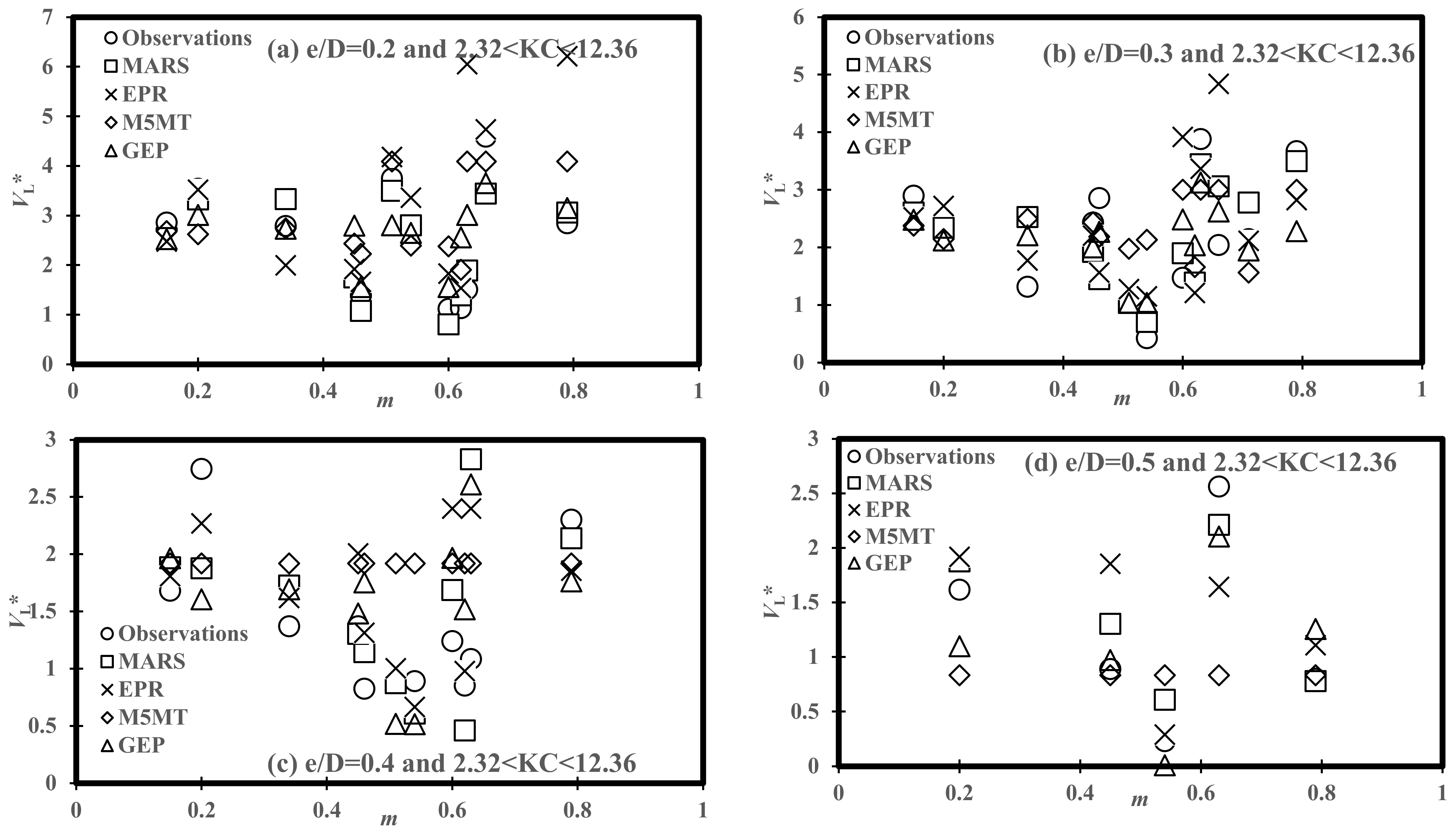
- The physical consistency of the predictive models’ results has been studied by analyzing scour propagation rates versus the ratio of pipeline embedment depth and pipeline diameter (e/D), the ratio of current velocity to orbital velocity (m), and Keulegan–Carpenter number (KC). From variations of the scour propagation patterns versus m, it was found that scour propagation rates followed a decreasing trend for m = 0.2–0.6 and all ranges of e/D and KC, then; increased up to m = 0.8.
- -
- The effects of complexity level on the performance of AI models for 3D scour propagation rates was investigated. The EPR model was developed by Set 6 for the VH* prediction with complex expressions in comparison with M5MT and Equation (24) (MARS). Multivariate linear equations by M5MT were simpler than those obtained expressions by EPR and GEP models. Additionally, the EPR model provided VR* prediction with simpler mathematical structures than that developed by the GEP model [Equation (21)]. The sixth combination of input parameters has been applied to acquire a mathematical expression-based GEP model with three genes, indicating the lowest level of efficiency in the calibration stage in comparison with AI techniques. On the contrary, the MARS model with four dimensionless inputs (i.e., m θC,(1 − m)θW, 1 − e/D, KC) and the second-order polynomial had better performance in the calibration phase than linear equations by M5MT. Furthermore, explicit equations given by MARS and EPR models have lower complexity for the VL* estimation in comparison with the GEP model.
Author Contributions
Funding
Institutional Review Board Statement
Informed Consent Statement
Data Availability Statement
Acknowledgments
Conflicts of Interest
References
- Cheng, L.; Yeow, K.; Zang, Z.; Li, F. 3D scour below pipelines under waves and combined waves and currents. Coast. Eng. 2014, 83, 137–149. [Google Scholar] [CrossRef] [Green Version]
- Cheng, L.; Yeow, K.; Zhang, Z.; Teng, B. Three-dimensional scour below offshore pipelines in steady currents. Coast. Eng. 2009, 56, 577–590. [Google Scholar] [CrossRef]
- Adegboye, M.A.; Fung, W.-K.; Karnik, A. Recent Advances in Pipeline Monitoring and Oil Leakage Detection Technologies: Principles and Approaches. Sensors 2019, 19, 2548. [Google Scholar] [CrossRef] [PubMed] [Green Version]
- Sumer, B.M.; Fredsoe, J. The Mechanics of Scour in the Marine Environment; World Scientific: Singapore, 2002. [Google Scholar]
- Sumer, B.M.; FredsØe, J. Scour below pipelines in waves. J. Waterway Port Coast. Ocean Eng. 1990, 116, 307–323. [Google Scholar] [CrossRef]
- Sumer, B.M.; Truelsen, C.; Sichmann, T.; Fredsøe, J. Onset of scour below pipelines and self-burial. Coast. Eng. 2001, 42, 313–335. [Google Scholar] [CrossRef]
- Bernetti, R.; Bruschi, R.; Valentini, V.; Venturi, M. Pipelines placed on erodible seabeds. In Proceedings of the 9th International Conference on Offshore Mechanics and Artic Engineering, ASME, Houston, TX, USA, 18–23 February 1990; Volume 5, pp. 155–164. [Google Scholar]
- Lucassen, R.J. Scour Underneath Submarine Pipelines. In MAT Rep. PL-42A, Marine Tech. Res.; TU Delft: Delft, The Netherlands, 1984. [Google Scholar]
- Sumer, B.M.; Fredsøe, J. Scour around pipelines in combined waves and current. In Proceedings of the 15th Conference on Offshore Mechanics Arctic Engineering, Florence, Italy, 16–20 June 1996; American Society of Mechanical Engineers: New York, NY, USA, 1996; Volume 5, pp. 595–602. [Google Scholar]
- Fredsae, J.; Sumer, B.M.; Arnskov, M.M. Time scale for wave/current scour below pipelines. Int. J. Offshore Polar Eng. 1992, 2, 13–17. [Google Scholar]
- Wu, Y.; Chiew, Y.-M. Three-dimensional scour at submarine pipelines. J. Hydraul. Eng. 2012, 138, 788–795. [Google Scholar] [CrossRef]
- Wu, Y.; Chiew, Y.-M. Mechanics of three-dimensional pipeline scour in unidirectional steady current. J. Pipeline Syst. Eng. 2013, 4, 3–10. [Google Scholar] [CrossRef]
- Najafzadeh, M.; Saberi-Movahed, F. GMDH-GEP to predict free span expansion rates below pipelines under waves. Mar. Georesources Geotechnol. 2019, 37, 375–392. [Google Scholar] [CrossRef]
- Ehteram, M.; Ahmed, A.N.; Ling, L.; Fai, C.M.; Latif, S.D.; Afan, H.A.; Banadkooki, F.B.; El Shafie, A. Pipeline scour rates prediction-based model utilizing a Multilayer Perceptron-Colliding Body algorithm. Water 2020, 12, 902. [Google Scholar] [CrossRef] [Green Version]
- Najafzadeh, M.; Oliveto, G. Exploring 3D wave-induced scouring patterns around subsea pipelines with Artificial Intelligence techniques. Appl. Sci. 2021, 11, 3792. [Google Scholar] [CrossRef]
- Najafzadeh, M.; Oliveto, G. Scour Propagation Rates around Offshore Pipelines Exposed to Currents by Applying Data-Driven Models. Water 2022, 14, 493. [Google Scholar] [CrossRef]
- Hansen, E.A.; Staub, C.; Fredsøe, J.; Sumer, B.M. Time-development of scour induced free spans of pipelines. In Proceedings of the 10th Conference on Offshore Mechanics and Arctic Engineering (OMAE), Stavanger, Norway, 23–28 June 1991. [Google Scholar]
- Soulsby, R. Dynamics of Marine Sands: A Manual for Practical Applications; Thomas Telford: London, UK, 1997. [Google Scholar]
- Ferreira, C. Gene expression programming: A new adaptive algorithm for solving problems. Complex Syst. 2001, 13, 87–129. [Google Scholar]
- Ferreira, C. Gene Expression Programming, 2nd ed.; Springer: Berlin/Heidelberg, Germany, 2006. [Google Scholar]
- Friedman, J.H. Multivariate adaptive regression splines. Ann. Statist. 1991, 19, 1–67. [Google Scholar] [CrossRef]
- Mokhtia, M.; Eftekhari, M.; Saberi-Movahed, F. Feature selection based on regularization of sparsity based regression models by hesitant fuzzy correlation. Appl. Soft Comput. 2020, 91, 106255. [Google Scholar] [CrossRef]
- Mokhtia, M.; Eftekhari, M.; Saberi-Movahed, F. Dual-manifold regularized regression models for feature selection based on hesitant fuzzy correlation. Knowl.-Based Syst. 2021, 229, 107308. [Google Scholar] [CrossRef]
- Quinlan, J.R. Learning with Continuous Classes. In Proceedings of the 5th Australian Joint Conference on Artificial Intelligence (AI ’92); World Scientific: Singapore, 1992; pp. 343–348. [Google Scholar]
- Granata, F.; de Marinis, G. Machine learning methods for wastewater hydraulics. Flow Meas. Instrum. 2017, 57, 1–9. [Google Scholar] [CrossRef]
- Granata, F.; Saroli, M.; de Marinis, G.; Gargano, R. Machine learning models for spring discharge forecasting. Geofluids 2018, 2018, 8328167. [Google Scholar] [CrossRef] [Green Version]
- Solomatine, D.P.; Xue, Y. M5 Model Trees and Neural Networks: Application to Flood Forecasting in the Upper Reach of the Huai River in China. J. Hydrol. Eng. 2004, 9, 491–501. [Google Scholar] [CrossRef]
- Di Nunno, F.; Alves Pereira, F.; de Marinis, G.; Di Felice, F.; Gargano, R.; Miozzi, M.; Granata, F. Deformation of Air Bubbles Near a Plunging Jet Using a Machine Learning Approach. Appl. Sci. 2020, 10, 3879. [Google Scholar] [CrossRef]
- Granata, F.; Di Nunno, F. Air Entrainment in Drop Shafts: A Novel Approach Based on Machine Learning Algorithms and Hybrid Models. Fluids 2022, 7, 20. [Google Scholar] [CrossRef]
- Etemad-Shahidi, A.; Yasa, R.; Kazeminezhad, M.H. Prediction of wave-induced scour depth under submarine pipelines using machine learning approach. Appl. Ocean Res. 2011, 33, 54–59. [Google Scholar] [CrossRef] [Green Version]
- Giustolisi, O.; Doglioni, A.; Savic, D.A.; Webb, B.W. A multi-model approach to analysis of environmental analysis. Environ. Modell. Softw. 2007, 22, 674–682. [Google Scholar] [CrossRef] [Green Version]
- Giustolisi, O.; Savic, D.A. Advances in data-driven analyses and modelling using EPR-MOGA. J. Hydroinf. 2009, 11, 225–236. [Google Scholar] [CrossRef]
- Laucelli, D.; Giustolisi, O. Scour depth modeling by a multi-objective evolutionary paradigm. Environ. Model. Softw. 2011, 26, 498–509. [Google Scholar] [CrossRef]
- Savic, D.A.; Giustolisi, O.; Berardi, L.; Shepherd, W.; Djordjevic, S.; Saul, A. Modelling sewer failure by evolutionary computing. Water Manag. 2006, 159, 111–118. [Google Scholar] [CrossRef]
- Berardi, L.; Giustolisi, O.; Kapelan, Z.; Savic, D.A. Development of pipe deterioration models for water distribution systems using EPR. J. Hydroinf. 2008, 10, 113–126. [Google Scholar] [CrossRef] [Green Version]


| Set No. | List of Input Variables |
|---|---|
| Set 1 | e/D,KC,m,θW,θC |
| Set 2 | 1 − e/D,KC, (1 − m)θW + mθC |
| Set 3 | 1 − e/D,F, θW, θC |
| Set 4 | 1 − e/D, F, (1 − m)θW + mθC |
| Set 5 | e/D, F,m,θW,θC |
| Set 6 | 1 − e/D,KC, (1 − m)θW,mθC |
| Set 7 | 1 − e/D,KC, [(1 − m)θW + mθC]5/3 |
| Parameters | Data Range | Average | Standard Deviation | Coefficient of Variation |
|---|---|---|---|---|
| T (s) | 1–2 | 1.536 | 0.419 | 0.273 |
| UW (m/s) | 0.11–0.34 | 0.261 | 0.074 | 0.284 |
| E (cm) | 0.5–2.5 | 1.57 | 0.586 | 0.3717 |
| u* (m/s) | 0.0036–0.0282 | 0.0171 | 0.00769 | 0.449 |
| UC (m/s) | 0.06–0.47 | 0.291 | 0.130 | 0.445 |
| VH (mm/s) | 0.33–4.55 | 1.669 | 0.893 | 0.535 |
| m | 0.15–0.79 | 0.505 | 0.187 | 0.371 |
| θW | 0.0278–0.1315 | 0.08057 | 0.03094 | 0.361 |
| θC | 0.00048–0.0297 | 0.01356 | 0.00908 | 0.669 |
| KC | 2.2–13.6 | 8.314 | 3.723 | 0.448 |
| e/D | 0.2–0.5 | 0.319 | 0.102 | 0.319 |
| VH* | 0.26–3.61 | 1.326 | 0.709 | 0.535 |
| VR* | 0.609–7.9023 | 2.411 | 1.371 | 1.634 |
| VL* | 0.233–4.59 | 1.952 | 1.036 | 0.6023 |
| Set No. | VH* | VR* | VL* | |||
|---|---|---|---|---|---|---|
| Calibration | Validation | Calibration | Validation | Calibration | Validation | |
| 1 | 0.5921 | 0.748 | 0.6482 | 0.8345 | 0.6115 | 0.4135 |
| 2 | 0.6739 | 0.5056 | 0.5175 | 0.5768 | 0.5692 | 0.6290 |
| 3 | 0.7481 | 0.6118 | 0.6160 | 0.7913 | 0.5090 | 0.6619 |
| 4 | 0.6151 | 0.8933 | 0.59359 | 0.8438 | 0.6587 | 0.7778 |
| 5 | 0.7796 | 0.7029 | 0.6755 | 0.6251 | 0.7823 | 0.7071 |
| 6 | 0.7185 | 0.8477 | 0.6645 | 0.7425 | 0.73617 | 0.6746 |
| 7 | 0.4607 | 0.4867 | 0.46055 | 0.6911 | 0.7552 | 0.7833 |
| Parameters | Description of Parameters | Setting of Parameters |
|---|---|---|
| P1 | Function set | +, −, ×, /, Power (x2), (1 − x), 1/x, Average (x1,x2), Atan (x), 3Rt, Ln, Min |
| P2 | Linking function | Addition |
| P3 | Mutation rate | 0.00138 |
| P4 | Inversion rate | 0.00546 |
| P5 | One-point and two-point recombination rates | 0.00277 |
| P6 | Gene recombination rate | 0.00277 |
| P7 | Permutation | 0.00546 |
| P8 | Maximum tree depth | VH* (6), VR* (5), VL* (4) |
| P9 | Number of gene | 3 |
| P10 | Number of chromosomes | 30 |
| P11 | Number of generation | VH* (1364), VR* (861), VL* (3916) |
| P12 | Best fitness value | VH* (557.26), VR* (466.89), VL* (578.77) |
| Set No. | VH* | VR* | VL* | |||
|---|---|---|---|---|---|---|
| Calibration | Validation | Calibration | Validation | Calibration | Validation | |
| 1 | 0.837 | 0.558 | 0.8113 | 0.4777 | 0.6361 | 0.44 |
| 2 | 0.7705 | 0.7513 | Nan | Nan | Nan | Nan |
| 3 | 0.8370 | 0.5586 | 0.3945 | 0.5965 | 0.6144 | 0.4405 |
| 4 | 0.6142 | 0.5622 | 0.3945 | 0.5965 | 0.7744 | 0.4408 |
| 5 | 0.7943 | 0.4148 | 0.7392 | 0.2263 | 0.6835 | 0.5542 |
| 6 | 0.7578 | 0.6955 | 0.7325 | 0.5903 | 0.8439 | 0.8949 |
| 7 | 0.4396 | 0.6438 | 0.8475 | 0.3638 | 0.6317 | 0.7374 |
| Basis Functions Used in the Prediction of VH* | |
|---|---|
| BF1 | max(0, 0.61751 − F) |
| BF2 | max(0, 0.11276 − (1 − m)θW − mθC) |
| BF3 | max(0, 0.73254 − (1 − e/D)) |
| BF4 | max(0, 0.7 − (1 − e/D)) × max(0, F − 0.30369) |
| Basis functions used in the prediction of VR* | |
| BF1 | max(0, mθC − 0.03862) |
| BF2 | max(0, mθC − 0.064886) |
| BF3 | max(0, 0.064886 − mθC) |
| BF4 | max(0, 6.3 − KC) |
| BF5 | max(0, 0.7 − (1 − e/D)) × max(0, 0.078754 − ((1 − m)θW)) |
| BF6 | max(0, (1 − e/D) − 0.6) × max(0, (1 − m)θW − 0.068215 ) |
| Basis functions used in the prediction of VL* | |
| BF1 | max(0, mθC − 0.03044) |
| BF2 | max(0, 0.7 − (1 − e/D)) |
| BF3 | max(0, 0.0478720 − (1 − m)θW) |
| BF4 | max(0, (1 − m)θW − 0.0478720)×max(0, mθC − 0.017761) |
| Set No. | VH* | VR* | VL* | |||
|---|---|---|---|---|---|---|
| Calibration | Validation | Calibration | Validation | Calibration | Validation | |
| 1 | 0.65 | 0.75 | 0.361 | 0.681 | 0.4866 | 0.6394 |
| 2 | 0.434 | 0.5962 | 0.361 | 0.680 | 0.4866 | 0.6394 |
| 3 | 0.756 | 0.775 | 0.361 | 0.680 | 0.486 | 0.639 |
| 4 | 0.4409 | 0.5960 | 0.7887 | 0.670 | 0.4866 | 0.6394 |
| 5 | 0.765 | 0.781 | 0.745 | 0.7956 | 0.6794 | 0.7740 |
| 6 | 0.753 | 0.774 | 0.723 | 0.820 | 0.6916 | 0.7760 |
| 7 | 0.4339 | 0.596 | 0.361 | 0.681 | 0.4944 | 0.6440 |
| Rules of M5MT#1 with Focusing on Pruning and Smoothing Phases |
|---|
| Rule: 1 IF e/D < = 0.35 θC < = 0.087 THEN VH* = −5.6911 × θW + 27.9909 × θC − 6.8389 × m−2.8633 × e/D + 6.0401 Rule: 2 IF e/D > 0.35 THEN VH* = −6.015 × e/D + 4.3233 Rule: 3 VH* = +4.5309 |
| Rules of M5MT#1 with Focusing on Pruning and Smoothing Phases |
|---|
| Rule: 1 IF θC < = 0.087 THEN VR*= −4.3517 × θW + 17.5692 × θC − 6.868 × m − 6.0857 × e/D + 7.0983 THEN VR*= −9.5347 × e/D + 6.8673 |
| Rules of M5MT#1 with Focusing on Pruning and Smoothing Phases |
|---|
| Rule: 1 IF 1 − e/D > 0.65 mθC < = 0.052 THEN VL* = 2.4945 × (1 − e/D) + 8.6366 × (1 − m)θW + 8.5379 × mθC − 0.6196 Rule: 2 VL*= −10.8666 × (1 − e/D) − 4.5984 |
| Set No. | VH* | VR* | VL* | |||
|---|---|---|---|---|---|---|
| Calibration | Validation | Calibration | Validation | Calibration | Validation | |
| 1 | 0.7780 | 0.4137 | 0.7413 | 0.6800 | 0.79173 | 0.2661 |
| 2 | 0.6512 | 0.8881 | 0.5898 | 0.8194 | 0.6771 | 0.7373 |
| 3 | 0.6887 | 0.6018 | 0.7219 | 0.6467 | 0.8788 | 0.3685 |
| 4 | 0.6382 | 0.7297 | 0.5323 | 0.8396 | 0.6921 | 0.7264 |
| 5 | 0.6887 | 0.6031 | 0.7458 | 0.6651 | 0.8725 | 0.7853 |
| 6 | 0.8794 | 0.8842 | 0.7432 | 0.6556 | 0.7378 | 0.6403 |
| 7 | 0.6258 | 0.5769 | 0.5800 | 0.8285 | 0.6956 | 0.6735 |
| Soft Computing Models | Calibration Stage | ||||
|---|---|---|---|---|---|
| CC | RMSE | MAPE | SI | DR | |
| MARS (Developed by Set 2) | 0.770 | 0.987 | 0.398 | 0.424 | 1.167 |
| EPR (Developed by Set 6) | 0.879 | 0.595 | 0.224 | 0.256 | 1.046 |
| M5MT (Developed by Set 5) | 0.765 | 0.817 | 0.474 | 0.348 | 1.286 |
| GEP (Developed by Set 5) | 0.779 | 0.801 | 0.348 | 0.344 | 1.183 |
| Soft Computing Models | Validation Stage | ||||
| CC | RMSE | MAPE | SI | DR | |
| MARS (Developed by Set 2) | 0.751 | 0.929 | 0.498 | 0.516 | 0.897 |
| EPR (Developed by Set 6) | 0.884 | 1.509 | 0.796 | 0.832 | 0.927 |
| M5MT (Developed by Set 5) | 0.781 | 1.543 | 0.692 | 0.529 | 1.661 |
| GEP (Developed by Set 5) | 0.703 | 1.239 | 0.565 | 0.538 | 1.403 |
| Soft Computing Models | Calibration Stage | ||||
|---|---|---|---|---|---|
| CC | RMSE | MAPE | SI | DR | |
| MARS (Developed by Set 6) | 0.732 | 1.041 | 0.388 | 0.408 | 1.111 |
| EPR (Developed by Set 5) | 0.746 | 1.003 | 0.308 | 0.393 | 1.120 |
| M5MT (Developed by Set 5) | 0.745 | 1.006 | 0.312 | 0.394 | 1.163 |
| GEP (Developed by Set 6) | 0.664 | 1.142 | 0.373 | 0.447 | 1.174 |
| Soft Computing Models | Validation Stage | ||||
| CC | RMSE | MAPE | SI | DR | |
| MARS (Developed by Set 6) | 0.590 | 0.981 | 0.384 | 0.446 | 1.632 |
| EPR (Developed by Set 5) | 0.665 | 2.236 | 0.764 | 0.878 | 1.234 |
| M5MT (Developed by Set 5) | 0.795 | 1.388 | 0.581 | 0.527 | 1.415 |
| GEP (Developed by Set 6) | 0.742 | 1.142 | 0.315 | 0.223 | 1.259 |
| Soft Computing Models | Calibration Stage | ||||
|---|---|---|---|---|---|
| CC | RMSE | MAPE | SI | DR | |
| MARS (Developed by Set 6) | 0.844 | 0.602 | 0.314 | 0.286 | 1.108 |
| EPR (Developed by Set 5) | 0.872 | 0.544 | 0.290 | 0.259 | 1.129 |
| M5MT (Developed by Set 6) | 0.691 | 0.807 | 0.598 | 0.383 | 1.374 |
| GEP (Developed by Set 7) | 0.755 | 0.739 | 0.447 | 0.352 | 1.144 |
| Soft Computing Models | Validation Stage | ||||
| CC | RMSE | MAPE | SI | DR | |
| MARS (Developed by Set 6) | 0.895 | 0.440 | 0.248 | 0.253 | 1.139 |
| EPR (Developed by Set 5) | 0.785 | 2.203 | 0.991 | 0.991 | 1.991 |
| M5MT (Developed by Set 6) | 0.776 | 1.197 | 0.679 | 0.439 | 1.666 |
| GEP (Developed by Set 7) | 0.783 | 0.674 | 0.358 | 0.369 | 1.231 |
| Soft Computing Models | Variation of VH* vs. m for 2.32 < KC < 12.36 | |||
|---|---|---|---|---|
| e/D = 0.2 | e/D = 0.3 | e/D = 0.4 | e/D = 0.5 | |
| MARS | 0.943 | 1.251 | 0.696 | 0.563 |
| EPR | 0.947 | 1.038 | 0.812 | 0.390 |
| M5MT | 1.105 | 1.229 | 0.741 | 0.835 |
| GEP | 0.902 | 1.187 | 0.426 | 0.803 |
| Soft Computing Models | Variation of VR* vs. m for 2.32 < KC < 12.36 | |||
| e/D = 0.2 | e/D = 0.3 | e/D = 0.4 | e/D = 0.5 | |
| MARS | 1.029 | 1.141 | 1.061 | 0.495 |
| EPR | 1.366 | 1.721 | 1.326 | 0.439 |
| M5MT | 1.182 | 1.361 | 0.862 | 0.577 |
| GEP | 0.842 | 1.323 | 1.008 | 0.439 |
| Soft Computing Models | Variation of VL* vs. m for 2.32 < KC < 12.36 | |||
| e/D = 0.2 | e/D = 0.3 | e/D = 0.4 | e/D = 0.5 | |
| MARS | 0.437 | 0.671 | 0.642 | 0.318 |
| EPR | 1.685 | 1.157 | 0.623 | 0.626 |
| M5MT | 1.035 | 0.910 | 0.792 | 0.891 |
| GEP | 0.805 | 0.716 | 0.756 | 0.386 |
Publisher’s Note: MDPI stays neutral with regard to jurisdictional claims in published maps and institutional affiliations. |
© 2022 by the authors. Licensee MDPI, Basel, Switzerland. This article is an open access article distributed under the terms and conditions of the Creative Commons Attribution (CC BY) license (https://creativecommons.org/licenses/by/4.0/).
Share and Cite
Najafzadeh, M.; Oliveto, G.; Saberi-Movahed, F. Estimation of Scour Propagation Rates around Pipelines While Considering Simultaneous Effects of Waves and Currents Conditions. Water 2022, 14, 1589. https://doi.org/10.3390/w14101589
Najafzadeh M, Oliveto G, Saberi-Movahed F. Estimation of Scour Propagation Rates around Pipelines While Considering Simultaneous Effects of Waves and Currents Conditions. Water. 2022; 14(10):1589. https://doi.org/10.3390/w14101589
Chicago/Turabian StyleNajafzadeh, Mohammad, Giuseppe Oliveto, and Farshad Saberi-Movahed. 2022. "Estimation of Scour Propagation Rates around Pipelines While Considering Simultaneous Effects of Waves and Currents Conditions" Water 14, no. 10: 1589. https://doi.org/10.3390/w14101589
APA StyleNajafzadeh, M., Oliveto, G., & Saberi-Movahed, F. (2022). Estimation of Scour Propagation Rates around Pipelines While Considering Simultaneous Effects of Waves and Currents Conditions. Water, 14(10), 1589. https://doi.org/10.3390/w14101589