
Flood Forecasting via the Ensemble Kalman Filter Method Using Merged Satellite and Measured Soil Moisture Data


1
Key Laboratory of Groundwater Conservation of MWR, China University of Geosciences (Beijing), Beijing 100083, China
2
School of Water Resources & Environment, China University of Geosciences (Beijing), Beijing 100083, China
3
Key Laboratory of Simulation and Regulation of Water Cycle in River Basin, China Institute of Water Resources and Hydropower Research, Beijing 100038, China
4
Huairou District Scientific and Technical Committee, Beijing 101400, China
*
Author to whom correspondence should be addressed.
Water 2022, 14(10), 1555; https://doi.org/10.3390/w14101555
Submission received: 18 April 2022
/
Revised: 28 April 2022
/
Accepted: 9 May 2022
/
Published: 12 May 2022
(This article belongs to the Special Issue Water and Soil Resources Management in Agricultural Areas)
Abstract
:Flood monitoring in the Chaohe River Basin is crucial for the timely and accurate forecasting of flood flow. Hydrological models used for the simulation of hydrological processes are affected by soil moisture (SM) data and uncertain model parameters. Hence, in this study, measured satellite-based SM data obtained from different spatial scales were merged, and the model state and parameters were updated in real time via the data assimilation method named ensemble Kalman filter. Four different assimilation settings were used for the forecasting of different floods at three hydrological stations in the Chaohe River Basin: flood forecasting without data assimilation (NA case), assimilation of runoff data (AF case), assimilation of runoff and satellite-based soil moisture data (AFWR case), and assimilation of runoff and merged soil moisture data (AFWM case). Compared with NA, the relative error (RE) of small, medium, and large floods decreased from 0.53 to 0.23, 0.35 to 0.16, and 0.34 to 0.12 in the AF case, respectively, indicating that the runoff prediction was significantly improved by the assimilation of runoff data. In the AFWR and AFWM cases, the REs of the small, medium, and large floods also decreased, indicating that the soil moisture data play important roles in the assimilation of medium and small floods. To study the factors affecting the assimilation, the changes in the parameter mean and variance and the number of set samples were analyzed. Our results have important implications for the prediction of different levels of floods and related assimilation processes.
1. Introduction
Hydrological models are used for the simulation of various hydrological processes over an extended period of time [1,2,3]. However, the uncertainty of the model parameters and input data, such as soil moisture (SM) [4] data, leads to inaccurate simulation results [5]. The higher the accuracy of the model parameters, the greater the fit between the simulation results and real data. During runoff generation, SM regulates the magnitude of the flood with respect to the precipitation input via the partition of precipitation into runoff [6,7]. Wood [8] used the Kalman filter (KF) to recursively estimate the response function of the rainfall runoff system, analyzed the short-term structure and parameter changes using a hydrological prediction model, and achieved good results. However, the KF is only suitable for linear systems, not for complex nonlinear systems, and the adjoint mode calculation is very large. Therefore, an extended Kalman filter (EKF) [9] was developed, but it requires a tangent linear model and the final estimate is suboptimal. In the mid-1990s, the idea of the ensemble Kalman filter (EnKF) [10] emerged. Whitaker and Hamill [11] proposed an EnKF without disturbance observation and proved the advantages of the assimilation effect of this method. As the EnKF method is based on set statistics, the tangent and adjoint modes do not have to be calculated—wherein computation and time are saved—and the modularity can easily be programmed and modified. Simultaneously, various uncertainties are considered and observation data are introduced to update and correct state variables in real time, thus improving the prediction accuracy. Therefore, this method has become popular in data assimilation research.
Floods occur due to natural factors, including precipitation, insufficient volume in banks or rivers, and riverbed deposition [12]. Therefore, it is very important to predict the flood flow and duration in time and accurately in order to prevent a disaster caused by flooding [13]. The aim of this study was to couple the hydrological model and EnKF to improve the accuracy of flood forecasting. Generally, the parameters of the applied hydrological model are certain, but the underlying surface conditions of the actual watershed often change (e.g., land use) due to climate change and frequent human activities. These changes will alter the physical characteristics of the watershed (i.e., runoff process and river routing). The parameters of the applied hydrological model are not static and will dynamically change with the environment. The model must also be adapted to the parameters, which change with the variables with time. Therefore, it is necessary to simultaneously assimilate the estimated parameters and variables. The model has been applied to hydrological forecasting. Moradkhani et al. [14] firstly studied the assimilation of the parameters and variables of a conceptual precipitation–runoff hydrological model by using the EnKF algorithm and proved that the synchronous estimation of parameters and variables reduces the uncertainty and improves the forecasting accuracy. In the same year, it was also confirmed that the assimilation process of the EnKF synchronous estimation method can be used to detect time-varying parameters and minimize the short-term deviation. It has been reported that the disturbance amplitude affects the accuracy of the set size based on the adjustment of the super-parameter value [15]. Xie and Zhang [16] used the EnKF state variable expansion method to synchronously assimilate parameters and variables as joint variables and proved that this synchronous estimation method reduces the deviation of the parameters and variables. To further study the parameter sensitivity of assimilation, Xie and Zhang [17] used the EnKF algorithm to synchronously estimate the parameters and variables of the Zhanghe River Basin in China using a distributed hydrological model, classified the parameters based on the parameter sensitivity, and then predicted and updated them. They confirmed the improvement in the forecasting accuracy of the hydrological model. Lü et al. [18] used the EnKF to synchronously estimate and calculate the variables and sensitivity parameters of the Xin’anjiang precipitation runoff model. The comparison of the results obtained from assimilating only the parameters or only the variables showed that the runoff simulation results were better when both parameters and variables were assimilated. Shi. [19] tested the capability of the EnKF to simultaneously estimate multiple parameters of a hydrologic model using multivariate field observations. The results showed that the EnKF provides reliable model parameter estimates. Khaki et al. [20] used data assimilation to improve a hydrological model, and then compared the results with the state estimation and reported that the combination of simultaneous assimilation and parameter estimation greatly improves the model prediction. Therefore, the EnKF algorithm was used to solve the problem of parameter uncertainty and improve the prediction accuracy in this study.
For short-term flood forecasting, precipitation and SM data can be measured using meteorological and rural gas stations. As important input driving data of hydrological models, their accuracies play important roles in the results of flood forecasts [21]. Satellite technology can now be used to obtain a wide range of SM with high accuracy, thus providing more basic data for model operations [22]. However, satellite data are occasionally affected by climate and data cannot be captured under cloud cover. Therefore, in this study, the SM data measured on the ground were merged with satellite data to improve the comprehensiveness and accuracy of the data and further improve the model prediction.
The supplementation of SM data also improves the accuracy of flood forecasting. Thus, it is of great significance to introduce runoff and SM data for multi-source data assimilation. Lee [23] confirmed that the use of the EnKF algorithm to assimilate in situ SM data based on the assimilation of runoff significantly improves the runoff and SM prediction. Dumedah and Coulibaly [24] also concluded that the assimilation of SM data has the potential to improve the runoff accuracy. Samuel [25] reported that the assimilation effect is poor when only the runoff and soil water content are assimilated with the EnKF algorithm, whereas the best effect was achieved by assimilating both the runoff and soil water content. Liu [26] studied the upper reaches of the Huaihe River by coupling the EnKF and Swat models, synchronously estimated the variables and parameters, and investigated the effects of surface SM data on the assimilation. The results proved that adding SM data improves both the effective SM and the runoff estimation.
2. Materials and Methods
2.1. Study Area
The map of the Chaohe River Basin, including the digital elevation model (DEM), basin boundary, and locations of hydrological and precipitation stations, is shown in Figure 1. The river basin is located in the Miyun District of Beijing, China. The river originates in Fengning County, Chengde City, Hebei Province, and flows into the Miyun Reservoir in the south. It is an important branch of the Haihe River. The regulation and storage capacity of the Choate River Basin changed in the 1980s due to social and economic activities and the construction of water conservancy facilities, and the natural runoff sequence has lost consistency. Therefore, accurate flood forecasting is crucial for the Chaohe River Basin. The basin is located between 40°19′–41°38′ N and 116°7′–117°35′ E, covering an area of 6277.5 km2. The annual average runoff is 200 million m3. The Chaohe River Basin is mainly mountainous and hilly, with a warm, temperate, monsoon, continental, semi-humid, and semi-arid climate, and rainfall is mainly concentrated from June to September. The annual average temperature ranges from 9 to 10 °C. The annual average precipitation is 502 mm and the annual runoff distribution is uneven. Rainfall is abundant in summer and autumn, whereas less rainfall occurs in spring and winter. The flood season is June–October, accounting for 66% of the year [27]. The Chaohe River Basin contains three hydrological and 15 precipitation stations. From upstream to downstream, the hydrological stations are the Dage, Gubeikou, and Xiahui stations. The control areas of the Dage, Gubeikou, and Xiahui stations are 1898, 4484, and 5128 km2, respectively.
2.2. Data
Due to the lack of SM data in recent years, precipitation, evaporation, runoff, and SM data from 2000 to 2005 were used in this study.
2.2.1. Precipitation and Runoff Data
The Chaohe River Basin in the Miyun area of Beijing was selected as the study area. Basic data regarding this basin include daily precipitation, daily runoff, and daily evaporation data from 2000 to 2005. The daily precipitation data were obtained from 15 rain gauges in the basin. The daily runoff data were recorded at three hydrological stations. Evaporation information was derived from daily pan evaporation data. The data were used for the parameter calibration and multisource data assimilation.
2.2.2. Soil Moisture Data
The SM directly affects the surface runoff and evapotranspiration data of the watershed; therefore, assimilated observations of the soil water capacity can significantly improve the estimation of the SM, runoff, and evapotranspiration, reducing the uncertainty in hydrological model predictions [28]. The satellite soil data in this study are based on the daily SM dataset of the European Space Agency (ESA) Climate Change Initiative (CCI) SM combination product. The CCI project is an important part of the basic climate parameter monitoring project of the ESA. Active and passive microwave remote sensing SM data are combined, forming a complete and unified global SM dataset (ESA CCI SM) [29]. Some satellite-based SM are missing and supplemented by interpolation. The measured SM data, which contain ten-day datasets of the crop growth and development and the farmland SM, were obtained from the China Agrometeorological Data Station. The soil relative humidity values were measured at multiple depths. However, only the soil relative humidity values observed at a depth of 10 cm were used for consistency with remote sensing data.
2.3. Improved Xin’anjiang Model
Based on the climatic characteristics and geographical conditions of the Chaohe River Basin, the improved Xin’anjiang model [30] (four water sources, super-infiltration, and full storage) was used in this study. The calculation of runoff yield adopts the combination of full storage runoff yield and super-infiltration runoff yield. When calculating river basin routing, different water sources use different routing methods. Surface water uses the dimensionless unit hydrograph method, and soil water and groundwater use the linear reservoir method. After the improvement, the model contained 21 variable parameters. The symbols, physical meanings, and upper and lower limits of parameters are shown in Table 1. The particle swarm optimization algorithm [31], with high precision and fast convergence, was used for the parameter calibration in this study. The global sensitivity analysis method LH-OAT [32,33] was used to analyze the sensitivity of the 21 model parameters. The analysis results are shown in Figure 2. Four parameters, the IMP, SM, K, and B, are extremely sensitive. The SM and B were selected as updated parameters in the data assimilation method.
3. Methods
3.1. Data Merging
Satellite and measured SM data are inconsistent due to systematic errors. The cumulative distribution function (CDF) [34] method was adopted to achieve a better match between the two groups of data. The CDF can be used to describe a random variable X, which is the integral of the probability density function—that is, the probability P that a random variable is lower than or equal to a certain value. Based on CDF matching technology, the measured SM data are used to correct the satellite SM data. Thus, the two data groups have the same value range and cumulative probability distribution value and the overall deviation is corrected. The CDF matching technique is based on piecewise linear matching. The adjusted CCI SM and SM measured at the station satisfy the following expression:
where fCCI (x) and fmea (x1) represent the cumulative distribution function of the CCI SM and site SM, respectively, and X is the SM of unadjusted CCI products.
Taking the Dage station as an example, the measured and CCI satellite SM values from 2000 to 2005 were known and the CDF was adjusted as follows. First, the CDF curves of the two groups of data were drawn and divided into 12 segments, with the y-axis representing the percentage of the CDF—that is, 0, 5, 10, 20, 30, 40, 50, 60, 70, 80, 90, 95, and 100%. The CDF curves of the satellite and measured SM data are shown in Figure 3a,b, respectively. Second, the relationship between the satellite and measured SM data was plotted and the piecewise linear regression curve was obtained, as shown in Figure 3c. Thereby, the linear regression equation corresponding to each segment was obtained. Finally, the obtained linear regression equation was used to adjust the CDF and three groups of CDF curves were obtained—that is, satellite, measured, and merged SM CDF curves—as shown in Figure 3d.
3.2. Ensemble Kalman Filter (EnKF)
The EnKF [35] is a data assimilation technique that originated from the integration of the Kalman filter theory and Monte Carlo estimation. The goal of this sequential data assimilation approach is to update the model predictions by the optimal merging of the observations. The basic idea is to estimate the covariance between state and observation variables based on the results of the prediction set. The set average of the prediction state can be used as the best estimate and the sample covariance can be used as the approximation of the prediction error covariance. Based on continuous forward filtering, the analysis variables are updated using the observation data and covariance. The updated sample average of the analysis variable can be used as the best estimate of the variable.
The EnKF algorithm includes two processes—model state prediction and updating state variables with observed data [36,37]:
where and represent the state vector predicted by the model of the ith member of the set at time t + 1 and the state vector assimilated and updated at time t, respectively, f(.) is the model operator, is the model parameter vector of the assimilation update, is the model error term, is the error term of boundary conditions, and is the model’s external force field.
To simultaneously estimate variables and parameters, it is necessary to change the state vector in Equation (2) to include the parameters of the model:
- Observation data update
The state variables were filtered and updated using the observation data:
where represents the observed data, which are generally obtained after adding Gaussian perturbation; is an observation operator whose function can map the extended state vector predicted by the model into the observation space; and is Kalman gain, which is also known as the weight matrix and can be expressed as follows:
where is the covariance matrix of the observation data error. As the observation data were known, this was directly calculated with the equation, which is mainly used to quantify the uncertainty of observation data. The parameter is the prediction error covariance matrix, which expresses the correlation between observed variables and model parameters. This correlation was used for the simultaneous update of the dynamic variables and parameters without observation after adding the observation data. The specific expression is as follows:
3.3. Data Assimilation Setup
Four different assimilation settings were used to monitor the performance of multivariate data assimilation for flood events at three hydrological stations in the Chaohe River Basin. The measured daily precipitation, daily evaporation data, satellite SM data, and merged SM data from 2000 to 2005 were utilized to analyze the multivariate data assimilation. The flood level was divided into small, medium, and large floods according to the return period or frequency. Small and medium floods were selected for Dage Station and three floods of different grades were selected for the Gubeikou and Xiahui stations. Four different assimilation settings were used: non-assimilation value of the runoff without observation data (NA), single variate assimilation with runoff only (AF), multivariate assimilation with runoff and remote sensing SM data (AFWR), and multivariate assimilation with runoff and corrected SM data (AFWM).
The two-parameter variable Xin’anjiang model was used for the assimilation in this study. The two sensitivity parameters, SM (average free water storage capacity of the basin, mm) and B (soil storage capacity curve index), as well as the state variables S (average free water storage capacity of the basin, mm) and Q (simulated flow at the outlet of the basin, m3/s), which change with time, and the SM data W0 (1) (upper SM data, mm) were used as multi-source data. When only the runoff is assimilated, the expression of the state variable is X = (S, Q, SM, B)T and the observational operator is H = (0, 1, 0, 0)T. After adding the SM data W0 (1) of multi-source data, the state variable can be expressed as X = (S, Q, W0(1), SM, B)T and the observational operator is H = (0, 1, 1, 0, 0)T. The distribution of the variables and parameters satisfies the Gaussian distribution. In addition, this assimilation experiment considered the uncertainty of the model itself and that of observation data. Both the model and observation errors obey a Gaussian distribution, and Gaussian white noise was used as the mean value of zero. The standard deviation, expressed as the scaling factor [38], was set to N (0, 0.12) and N (0, 0.12). The initial number of data assimilation sets was 200.
4. Results and Discussion
The simulation effect of the improved Xin’anjiang model can be tested with the Nash–Sutcliffe efficiency coefficient (NSE). The NSE ranges from −∞ to 1. The closer NSE is to 1, the better is the simulation effect. The closer NSE is to 0, the closer are the simulation results to the average of the measured values, indicating that the simulation results are overall credible but the simulation error is large. If the NSE is much lower than zero, the error is large and the model is not credible. The perfect NSE value is 1. The specific calculation equation is as follows:
where is the observation value at time t, is the flow simulation value at time t, and is the mean of the observation streamflow sequence.
The improved runoff was obtained by the application of the improved Xin’anjiang model to daily precipitation and daily evaporation data. Taking the Xiahui Hydrological Station as an example, the flood levels were divided based on the return period or frequency. The NSE values were 0.67, 0.48, and 0.3, respectively. The results indicated that the simulation effect of the improved Xin’anjiang model was optimal.
4.1. Data Merging
Figure 4 compares the SM data after merging with the previous two types of SM data. Most of the satellite SM data before adjustment were lower than the SM data measured at the agricultural gas station, and the merged SM increased after the measured SM adjustment, implying that data merging yields data closer to the measured SM and improves the authenticity of the data. To compare the errors before and after adjustment, the average AE, RE, and RMSE values before and after adjustment are shown in Table 2. The error of the merged SM was significantly lower than that of the satellite SM data. The average AE, RE, and RMSE values decreased by 1.6%, 6.7%, and 0.41%, respectively, indicating that the merged soil data had higher quality than the original data. Therefore, the accuracy of the SM data of the Dage Hydrological Station improved after the CDF adjustment.
4.2. Data Assimilation
4.2.1. Small Flood
Figure 5 shows the variation in the flood runoff of small floods for the measurement and four assimilation settings. Among the three hydrological stations, the runoff of AF was closer to the measured runoff than that of NA, indicating that the assimilation effect was better than that of NA. The multi-source assimilation with runoff and SM data was closer to the measured runoff than that of AF. The AFWM was the closest to the measured runoff value, indicating that the multi-source assimilation effect was better and the merged SM data had the best effect.
The average error values of the four assimilation settings are shown in Table 3. At the Dage Hydrological Station, the average AE and RE values of AF decreased by 50.6% and 14.9%, respectively, compared with NA. The AE of AF was the lowest, but the multi-source assimilation effect of the runoff and SM data on the RE was better and AFWM was better than AFWR. Compared with runoff and satellite data, the AE and RE of the added runoff and merged SM data decreased by 4.8% and 4.8%, respectively. At the Gubeikou Hydrological Station, the average AE and RE values of AF decreased by 196% and 28.4%, respectively, compared with NA. The multi-source assimilation effect including runoff and SM data was better. The AE and RE values of AFWR decreased by 5.3% and 7.5%, respectively, and the AE and RE values of AFWM decreased by –1.3% and 5.8%, respectively. At the Xiahui Hydrological Station, the average AE and RE values of AF decreased by 28.1% and 6.8%, respectively, compared with NA. The RE of AFWR decreased by 13% compared with AF, and the AE of AFWM decreased by 3.9% compared with AFWR.
To understand the RE of the assimilation effect under different conditions, the RE value was plotted. Figure 6 shows the RE values under the four assimilation settings for the three stations, indicating that the assimilation improved the prediction accuracy and that the addition of runoff and merged SM data yielded the best effect.
4.2.2. Medium Flood
Figure 7 shows the variation in the flood runoff associated with medium floods for the measurement and four assimilation settings. Figure 7a shows that the runoff of AF at the Dage Hydrological Station was closer to the measured runoff value than NA, indicating that the assimilation had a significant effect. Compared with AF, the value obtained from multi-source assimilation including runoff and SM data was closer to the measured runoff value, and the merged data were closer to the measured value than the satellite SM data, indicating that the effect of merged SM data was better. Figure 7b shows that the runoff of AF at the Gubeikou Hydrological Station was closer to the measured runoff value than that of NA, indicating that the effect of assimilation was better than that of NA and the multi-source assimilation including runoff and SM data yielded a value closer to the measured runoff compared with AF. The AFWM value was the closest to the measured runoff value, indicating that the multi-source assimilation effect was better and the merged SM data had the best effect. Figure 7c shows that the runoff of AF at Xiahui Hydrological Station was closer to the measured flow value than NA, indicating that the effect of the assimilation was better than that without assimilation. However, compared with AF, the multi-source assimilation including runoff and SM data was not close to the measured runoff value.
The average error values of the four assimilation settings are shown in Table 4. At the Dage Hydrological Station, the average AE and RE values of AF decreased by 72.7% and 37.3%, respectively, compared with NA. The effect of adding multi-source soil data was better than AF, and the AE and RE values of AFWR decreased by 6.6% and 1.6%, respectively, compared with AF. The AFWM was better than AFWR. Compared with AFWR, the AE and RE values of AFWM decreased by 3.5% and 0.7%, respectively. At the Gubeikou Hydrological Station, the average RE values of AF decreased by 4.3%, compared with NA, and the AE of AF was lower than the error value obtained after adding SM data. Compared with AEWR, the AE and RE values of AFWM were reduced by 10.5% and 1.6%, respectively. At the Xiahui Hydrological Station, the average AE and RE values of AF decreased by 116% and 8.8%, respectively, compared with NA. The error of AF was lower than that after adding SM data. Overall, the effect of AF was better than that of adding SM data. The average AE and RE values of AF decreased by 153% and 18.5%, respectively, compared with AFWM. The merged data were better than the satellite data, and the AE of AFWM was reduced by 7.3% compared with that of the AFWR.
Figure 8 shows the RE values for medium floods for the four assimilation settings. It also shows that the assimilation improved the prediction accuracy and the effect of AFWM was better than that of AFWR.
4.2.3. Large Flood
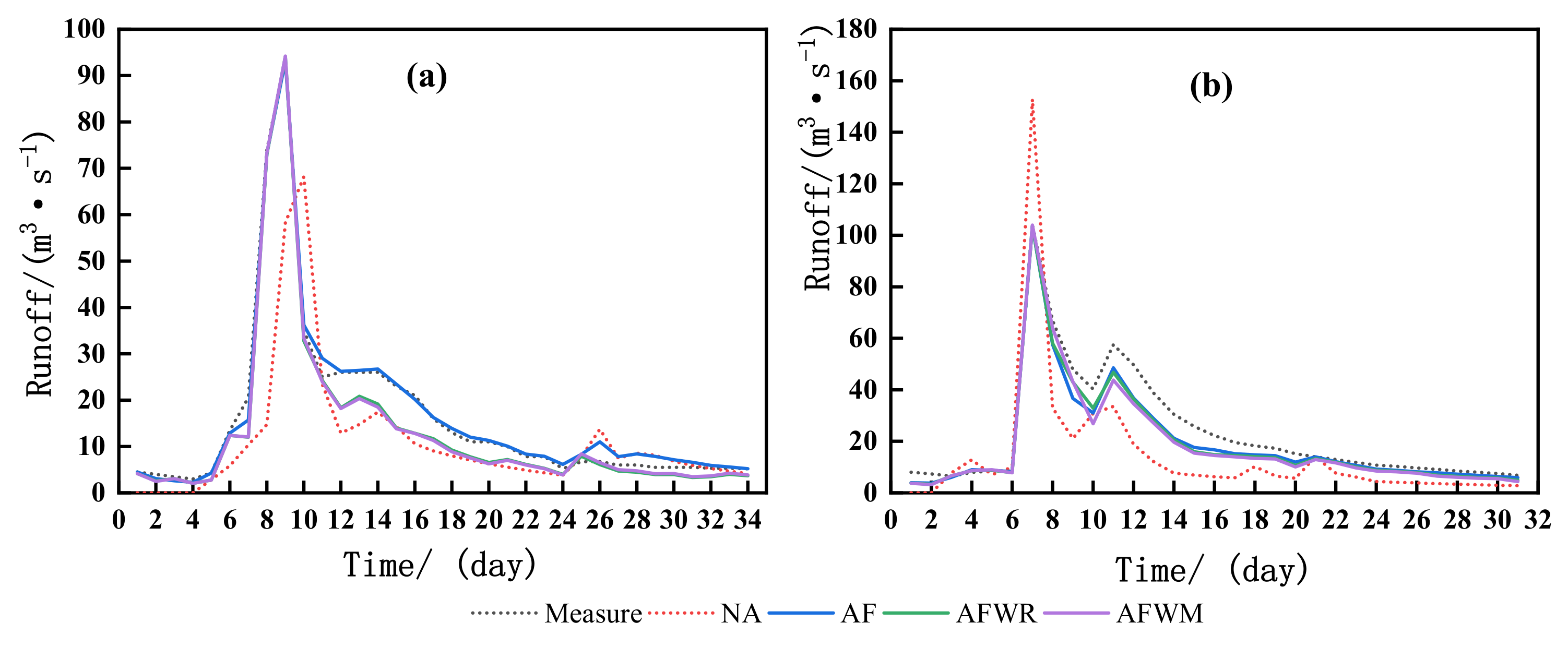
Due to the lack of large flood data recorded at the hydrological stations, the assimilation under the large flood level only included the Gubeikou and Xiahui stations. The variation in the flood runoff of large floods for the measurement and four assimilation settings is shown in Figure 9. Figure 9a shows that the runoff of AF at the Gubeikou Hydrological Station was closer to the measured runoff value than NA, but the multi-source assimilation including runoff and SM data was not close to the measured runoff value. The merged data were closer to the measured value than satellite SM data, indicating that the effect of the assimilation was better than that without assimilation, and the effect of merged SM data was better than that of satellite data. The results obtained for the Xiahui Hydrological Station are shown in Figure 9b.
The average error values of the four assimilation settings are shown in Table 5. At the Gubeikou Hydrological Station, the average RE value of AF decreased by 18.4% compared with NA. The RE value of AF was lower than that of SM data. Overall, the effect of assimilating only the runoff was better than that of SM data. The AE and RE values of AEWM decreased by 18.1% and 0.6%, respectively, compared with AEWR. At the Xiahui Hydrological Station, the average RE value of AF was 28.5% lower than that of NA and the average AE and RE values of AF were lower than those of the runoff with added SM data. For example, the average AE and RE values of AF were 29.9% and 3.5% lower than those of AFWR, respectively.
Figure 10 shows the RE values for large floods for the four assimilation settings. It also shows that the assimilation improved the prediction accuracy, but the multi-source assimilation effect of adding runoff and SM data was not as good as that of AF.
With respect to the evaluation of the assimilation effects of floods at different hydrological stations, Figure 11 shows that the RE of the simulation was notably reduced after the assimilation with measured data, indicating that the prediction effect of AF was better than that of NA. After the assimilation with soil data and runoff, the RE was worse than that obtained after assimilating only the runoff, indicating that the assimilation effect was less affected by SM data. Based on the trends of the RE values observed at different hydrological stations, the assimilation effect obtained for the Dage station was better than that of the Gubeikou and Xiahui stations—that is, the assimilation accuracy of the upstream hydrological station was higher than that of the midstream and downstream stations. This may be due to the gradual accumulation of errors during the data measurement at downstream hydrological stations, resulting in a larger deviation of the measured values and a worse assimilation effect.
With respect to the assimilation effect of different levels of field floods, the prediction effect of AF was better than that of NA, as shown in Figure 12. For large and medium floods, the runoff increased with the increase in the average precipitation, as shown in Figure 12a,b. Compared with the SM data, the runoff had a notable effect on the assimilation. Therefore, compared with AF, the effect became worse after adding SM data. For small floods, the average precipitation was equivalent to the soil water capacity, as shown in Figure 12c. The soil water capacity had a significant effect on the assimilation in the early stage. Therefore, the assimilation effect after adding SM multivariate data was better than that of AF, and AFWM was better than AFWR. Overall, the assimilation effect of small floods was better than that of medium and large floods, indicating that SM data are more useful for small floods and that it is more meaningful to predict small floods in the Chaohe River Basin.
Many factors affect the assimilation process. In this section, we discuss the factors affecting the assimilation based on the mean value, variance of parameters, and number of aggregate samples. Two large floods at Gubeikou Station for which a better effect was obtained by assimilating only the runoff were selected for this analysis. Based on the parameter optimization calculation, the optimal reference values of the parameters SM and B and the state variable S were 17.94 mm, 0.3, and 2 mm, respectively. The parameter SM was selected for further research. Based on the assumption that the distributions of the variables and parameters satisfied the Gaussian distribution, we used the following assimilation settings: SM~N (15, 52), B~N (0.2, 0.12), and S~N (5, 22).
The variance of the distribution of parameter SM was kept constant and the mean value was gradually changed. Therefore, the mean value gradually approached the initial true value (17.94 mm): 10, 12, 15, and 17 mm. The absolute error variation of the assimilation under different mean values is shown in Figure 13. When the mean value gradually increased from 10 to 17 mm and approached the initial true value of 17.94 mm, the AE between the final assimilated and measured runoff value continuously decreased. The error value was the lowest when the mean value was 17 mm and the average AE value of 17 mm was 155% lower than that of 10 mm. As the average value of the parameter gradually approached the true value of the parameter, the obtained parameter value was in the range of the true value. Therefore, it was possible to quickly obtain the optimal estimate during the assimilation and the assimilation efficiency improved. However, in the actual simulation, the true values of the parameters are unknown and must be calculated by formula derivation or relevant empirical models, which is the key direction of future research.
Similar to studying the effect of the mean value, the mean value of the distribution of parameter SM was kept constant and the variance was gradually changed: 52, 82, 102, and 202. The AE variation of the assimilation under different variance values is shown in Figure 14. With the increase in the variance, the AEs of the corresponding assimilated runoff and measured runoff values decreased first and then increased. The error value was the lowest when the variance was 102, and the AE with a variance of 102 was 7.6% lower than the average AE with a variance of 52. The AE with a variance of 102 was 7.7% lower than the average AE with a variance of 202. Therefore, if the variance of the assimilation parameters increased, the assimilation effect became better, because a larger variance reflects an enlarged extraction range, the true value could be easily covered, and the assimilation efficiency was improved. However, a larger variance setting results in a too wide range. In addition, the convergence time of the assimilation parameters will also increase, which is not conducive to the assimilation effect. Therefore, choosing an appropriate variance will improve the accuracy of the assimilation.
The number of sets was set to 50, 100, 200, and 250, whereas other conditions remained unchanged. The AE variation of the assimilation under different sample numbers is shown in Figure 15. With the increase in the number of sets, the AE value gradually decreased. When the number of sets was 50, the AE value was the largest and the assimilation effect was the worst. The AE value reached the minimum value when the number of sets was 200, which was very close to the value when the number of sets was 250. The average AE value at a number of sets of 200 was 133% lower than that of a number of sets of 50. Although the increase in the number of sets can accurately describe the distribution of the variables and parameters and the error value can be accurately calculated, the assimilation calculation time will increase when the number of sets increases. Therefore, the balance between the assimilation accuracy and calculation efficiency must be considered in the calculation process.
5. Conclusions
The aims of this study were to monitor the effect of the multivariate assimilation of floods in the Chaohe River Basin, improve the accuracy of the model simulation, timely and accurately forecast the flood flow, and prevent flood disasters. The EnKF was used for different assimilations of runoff and SM data.
The results of the analysis of the different flood levels indicated that the effect of the assimilation of multivariate runoff and SM data was better than that of AF for small floods in the basin. However, for medium and large floods, the assimilation effect of AF was better than that of multivariate data. Based on the RE values obtained at different hydrological stations, the assimilation effect of the Dage station was better than that of the Gubeikou and Xiahui stations. Overall, the assimilation effect differed for different levels of floods at different locations. The assimilation effect of small floods was better than that of medium and large floods. The assimilation accuracy obtained at upstream hydrological stations was higher than that obtained at stations in the midstream and lower reaches.
The analysis of four different assimilation conditions of flood events of different grades at different hydrological stations indicated that the prediction effect of the assimilation based on measured data was better than that of AF and the assimilation effect of merged SM data was better than that of satellite SM data.
Based on the analysis of various factors affecting the assimilation process, the effects of the mean, variance of the assimilation parameters, and number of sets on the assimilation results were determined. A mean parameter value close to the optimal value, appropriate increase in the variance, and moderate number of sets increase the accuracy of the runoff assimilation.
Furthermore, based on the combination of multivariate assimilation with the parameter estimation of runoff and SM data, good flood forecasts can be obtained. Therefore, it is important to estimate the model parameters during the data assimilation to improve the predictions. In general, based on the evaluation of the assimilation performance, multivariate data assimilation of the model parameters and variable estimation significantly improve the model simulation. In addition, with respect to the correlation between rain and floods in the north, the effect of the SM capacity can be clarified, laying a foundation for the prediction of short-term floods in the Chaohe River Basin.
However, due to the lack of SM data, it is impossible to make future predictions. The method should be tested in various basins with different hydroclimatic conditions to further evaluate its effect on the simulation. In addition, observed evapotranspiration should also be added to multi-source assimilation in the future, which would be more conducive to parameter estimation. Moreover, more uncertain parameters and corresponding error settings can be added to the EnKF method in the study.
Author Contributions
C.Z.: Methodology, Writing—Original draft preparation, Formal analysis, Validation, Visualization, Software; S.C.: Methodology, Investigation, Formal analysis, Validation, Software; J.T.: Supervision, Conceptualization, Methodology, Formal analysis, Resources, Data curation, Writing—Reviewing and Editing, Project administration, Funding acquisition; W.L.: Methodology, Investigation, Resources, Funding acquisition; P.Z.: Conceptualization, Methodology, Visualization, Formal analysis. All authors have read and agreed to the published version of the manuscript.
Funding
This work was partly supported by the National Natural Science Foundation of China (Grant 42072271), the National Key Research and Development Program of China (Grant 2021YFC3000205) and Key R&D Program of the China Huaneng Group Co., Ltd. (HNKJ20-H26).
Institutional Review Board Statement
Not applicable.
Informed Consent Statement
Informed consent was obtained from all subjects involved in the study. Written informed consent has been obtained from the patient(s) to publish this paper.
Data Availability Statement
The datasets generated and/or analyzed during the current study are not publicly available due to further dissertation writing but are available from the corresponding author on reasonable request.
Conflicts of Interest
The authors declare no conflict of interest.
Abbreviations
| NA | non-assimilation |
| AF | assimilation of runoff data |
| AFWR | assimilation of runoff and satellite-based soil moisture data |
| AFWM | assimilation of runoff and merged soil moisture data |
| RE | relative error |
| SM | soil moisture |
| KF | Kalman filter |
| EKF | extended Kalman filter |
| EnKF | ensemble Kalman filter |
| DEM | digital elevation model |
| ESA | European Space Agency |
| CCI | Climate Change Initiative |
| CDF | cumulative distribution function |
| NSE | Nash–Sutcliffe efficiency coefficient |
| AE | absolute error |
| RMSE | root-mean-square error |
References
- Bahrami, A.; Goïta, K.; Magagi, R.; Davison, B.; Razavi, S.; Elshamy, M.; Princz, D. Data assimilation of satellite-based terrestrial water storage changes into a hydrology land-surface model. J. Hydrol. 2020, 597, 125744. [Google Scholar] [CrossRef]
- Liu, Y.; Gupta, H.V. Uncertainty in hydrologic modeling: Toward an integrated data assimilation framework. Water Resour. Res. 2007, 43, W07401. [Google Scholar] [CrossRef]
- Abbott, M.B.; Refsgaard, J.C. Construction, calibration and validation of hydrological models. In Distributed Hydrological Modelling; Springer: Dordrecht, The Netherlands, 1990; pp. 41–54. [Google Scholar] [CrossRef]
- Alvarez-Garreton, C.; Ryu, D.; Western, A.W.; Su, C.H.; Crow, W.T.; Robertson, D.E.; Leahy, C. Improving operational flood ensemble prediction by the assimilation of satellite soil moisture: Comparison between lumped and semi-distributed schemes. Hydrol. Earth Syst. Sci. 2015, 19, 1659–1676. [Google Scholar] [CrossRef] [Green Version]
- Samuel, J.; Rousseau, A.N.; Abbasnezhadi, K.; Savary, S. Development and evaluation of a hydrologic data-assimilation scheme for short-range flow and inflow forecasts in a data-sparse high-latitude region using a distributed model and ensemble Kalman filtering. Adv. Water Resour. 2019, 130, 198–220. [Google Scholar] [CrossRef]
- Zhu, Q.; Wang, Y.; Luo, Y. Improvement of multi-layer soil moisture prediction using support vector machines and ensemble Kalman filter coupled with remote sensing soil moisture datasets over an agriculture dominant basin in China. Hydrol. Process. 2021, 35, e14154. [Google Scholar] [CrossRef]
- Azimi, S.; Dariane, A.B.; Modanesi, S.; Bauer-Marschallinger, B.; Bindish, R.; Wagner, W.; Massari, C. Understanding the benefit of Sentinel 1 and SMAP—Era satellite soil moisture retrievals for flood forecasting in small basins: Effect of revisit time and the spatial resolution. J. Hydrol. 2019, 581, 124367. [Google Scholar] [CrossRef]
- Wood, E.F.; Andras, S. An Adaptive Algorithm for Analyzing Short-Term Structural and Parameter Changes in Hydrologic Prediction Models. Water Resour. Res. 1978, 14, 577–581. [Google Scholar] [CrossRef]
- Aubert, D.; Loumagne, C.; Oudin, L. Sequential assimilation of soil moisture and streamflow data in a conceptual rainfall–runoff model. J. Hydrol. 2003, 280, 145–161. [Google Scholar] [CrossRef]
- Evensen, G. Sequential data assimilation with a nonlinear quasi-geostrophic model using Monte Carlo methods to forecast error statistics. J. Geophys. Res. Atmos. 1994, 99, 10143–10162. [Google Scholar] [CrossRef]
- Whitaker, J.S.; Hamill, T.M. Ensemble Data Assimilation without Perturbed Observations. Mon. Weather Rev. 2002, 130, 1913–1924. [Google Scholar] [CrossRef]
- Mehta, D.J.; Yadav, S.M. Hydrodynamic Simulation of River Ambica for Riverbed Assessment: A Case Study of Navsari Region. Lect. Notes Civ. Eng. 2020, 39, 127–140. [Google Scholar] [CrossRef]
- Wu, C.L.; Chau, K.W. Prediction of rainfall time series using modular soft computing methods. Eng. Appl. Artif. Intell. 2013, 26, 997–1007. [Google Scholar] [CrossRef] [Green Version]
- Moradkhani, H.; Sorooshian, S.; Gupta, H.V.; Houser, P.R. Dual state–parameter estimation of hydrological models using ensemble Kalman filter. Adv. Water Resour. 2005, 28, 135–147. [Google Scholar] [CrossRef] [Green Version]
- Moradkhani, H.; Hsu, K.L.; Gupta, H.; Sorooshian, S. Uncertainty assessment of hydrologic model states and parameters: Sequential data assimilation using the particle filter. Water Resour. Res. 2005, 41, 237–246. [Google Scholar] [CrossRef] [Green Version]
- Xie, X.H.; Zhang, D.X. Data assimilation for distributed hydrological catchment modeling via ensemble Kalman filter. Adv. Water Resour. 2010, 33, 678–690. [Google Scholar] [CrossRef]
- Xie, X.H.; Zhang, D.X. A partitioned update scheme for state-parameter estimation of distributed hydrologic models based on the ensemble Kalman filter. Water Resour. Res. 2013, 49, 7350–7365. [Google Scholar] [CrossRef]
- Lü, H.S.; Hou, T.; Horton, R.; Zhu, Y.H.; Chen, X.; Jia, Y.W.; Wang, W.; Fu, X.L. The streamflow estimation using the Xinanjiang rainfall runoff model and dual state-parameter estimation method. J. Hydrol. 2013, 480, 102–114. [Google Scholar] [CrossRef]
- Shi, Y.; Davis, K.J.; Zhang, F.; Duffy, C.J.; Yu, X. Parameter estimation of a physically-based land surface hydrologic model using an ensemble Kalman filter: A multivariate real-data experiment. Adv. Water Resour. 2015, 83, 421–427. [Google Scholar] [CrossRef] [Green Version]
- Khaki, M.; Hendricks Franssen, H.J.; Han, S.C. Multi-mission satellite remote sensing data for improving land hydrological models via data assimilation. Sci. Rep. 2020, 10, 18791. [Google Scholar] [CrossRef]
- Kampf, S.K.; Burges, S.J. Parameter estimation for a physics-based distributed hydrologic model using measured outflow fluxes and internal moisture states. Water Resour. Res. 2007, 43, 55–60. [Google Scholar] [CrossRef]
- Pan, M.; Wood, E.F.; Wójcik, R.; McCabe, M.F. Estimation of regional terrestrial water cycle using multi-sensor remote sensing observations and data assimilation. Remote Sens. Environ. 2008, 112, 1282–1294. [Google Scholar] [CrossRef]
- Lee, H.; Seo, D.J.; Koren, V. Assimilation of streamflow and in situ soil moisture data into operational distributed hydrologic models: Effects of uncertainties in the data and initial model soil moisture states. Adv. Water Resour. 2011, 34, 1597–1615. [Google Scholar] [CrossRef]
- Dumedah, G.; Coulibaly, P. Evolutionary assimilation of streamflow in distributed hydrologic modeling using in-situ soil moisture data. Adv. Water Resour. 2013, 53, 231–241. [Google Scholar] [CrossRef]
- Samuel, J.; Coulibaly, P.; Dumedah, G.; Moradkhan, H. Assessing model state and forecasts variation in hydrologic data assimilation. J. Hydrol. 2014, 513, 127–141. [Google Scholar] [CrossRef]
- Liu, Y.; Wang, W.; Hu, Y. Investigating the impact of surface soil moisture assimilation on state and parameter estimation in SWAT model based on the ensemble Kalman filter in upper Huai River basin. J. Hydrol. Hydromech. 2017, 65, 123–133. [Google Scholar] [CrossRef] [Green Version]
- Zhang, L.; Wang, G.L. Analysis on Error Distributions of Input Data and Output Data of Flood Forecasting Model and Its Correlation. J. China Hydrol. 2022, 42, 23–28. [Google Scholar] [CrossRef]
- Entekhabi, D.; Nakamura, H.; Njoku, E.G. Solving the inverse problem for soil moisture and temperature profiles by sequential assimilation of multifrequency remotely sensed observations. IEEE Trans. Geosci. Remote Sens. 1994, 32, 438–448. [Google Scholar] [CrossRef]
- Wagner, W.; Dorigo, W.; De Jeu, R.; Fernandez, D.; Benveniste, J.; Haas, E.; Ertl, M. Fusion of active and passive microwave observations to create an essential climate variable data record on soil moisture. In Proceedings of the ISPRS Annals of Photogrammetry, Remote Sensing and Spatial Information Sciences, Melbourne, Australia, 25 August–1 September 2012; pp. 315–321. [Google Scholar] [CrossRef]
- Li, Y.K.; Mao, F.; Li, M.Y.; Li, Y.G.; Peng, Y.X. Design flood revision method based on improved Xin’anjiang model—Taking Chaohe River Basin as an example. China Flood Drought Manag. 2021, 31, 49–54. [Google Scholar] [CrossRef]
- Eberhart, R.C.; Kennedy, J. A new optimizer using particle swarm theory. In Proceedings of the IEEE MHS’95—Sixth International Symposium on Micro Machine and Human Science, Nagoya, Japan, 4–6 October 1995; pp. 39–43. [Google Scholar] [CrossRef]
- Shi, Y.; Eberhart, R. A modified particle swarm optimizer. In Proceedings of the 1998 IEEE International Conference on Evolutionary Computation Proceedings, IEEE World Congress on Computational Intelligence (Cat. No.98TH8360), Anchorage, AK, USA, 4–9 May 1998; pp. 69–73. [Google Scholar] [CrossRef]
- Griensven, A.V.; Meixner, T.; Grunwald, S.; Bishop, T.; Diluzio, M.; Srinivasan, R. A global sensitivity analysis tool for the parameters of multi-variable catchment models. J. Hydrol. 2006, 324, 10–23. [Google Scholar] [CrossRef]
- Evensen, G. The ensemble Kalman filter: Theoretical formulation and practical implementation. Ocean. Dyn. 2003, 53, 343–367. [Google Scholar] [CrossRef]
- Kalman, R.E. A New Approach to Linear Filtering and Predietion Problems. Trans. ASME-J. Basic Eng. 1960, 82, 35–45. [Google Scholar] [CrossRef] [Green Version]
- Burgers, G.; Van Leeuwen, P.J.; Evensen, G. Analysis Scheme in the Ensemble Kalman Filter. Mon. Weather Rev. 1998, 126, 1719–1724. [Google Scholar] [CrossRef]
- Reichle, R.H.; Mclaughlin, D.B.; Entekhabi, D. Hydrologic Data assimilation with the ensemble Kalman filter. Mon. Weather Rev. 2000, 130, 103–114. [Google Scholar] [CrossRef] [Green Version]
- Xie, X.H.; Meng, S.; Liang, S.; Yao, Y. Improving streamflow predictions at ungauged locations with real-time updating: Application of an EnKF-based state-parameter estimation strategy. Hydrol. Earth Syst. Sci. 2014, 18, 13441–13473. [Google Scholar] [CrossRef] [Green Version]
Figure 1.
Map of the Chaohe River Basin including the digital elevation model (DEM), basin boundary, and locations of hydrological and precipitation stations.
Figure 1.
Map of the Chaohe River Basin including the digital elevation model (DEM), basin boundary, and locations of hydrological and precipitation stations.

Figure 2.
Scatter plot obtained from the sensitivity analysis.

Figure 3.
CDF curve for the (a) measured soil moisture; (b) satellite soil moisture; (c) piecewise linear regression; and (d) comparison before and after CDF adjustment.
Figure 3.
CDF curve for the (a) measured soil moisture; (b) satellite soil moisture; (c) piecewise linear regression; and (d) comparison before and after CDF adjustment.

Figure 4.
Time series curve of the soil moisture before and after adjustment.

Figure 5.
Variation in the flood runoff for small floods for the measurement and four assimilation settings for the three stations: (a) Dage; (b) Gubeikou; (c) Xiahui.
Figure 5.
Variation in the flood runoff for small floods for the measurement and four assimilation settings for the three stations: (a) Dage; (b) Gubeikou; (c) Xiahui.

Figure 6.
The RE values under the four assimilation settings for small floods for the three stations: (a) Dage; (b) Gubeikou; (c) Xiahui.
Figure 6.
The RE values under the four assimilation settings for small floods for the three stations: (a) Dage; (b) Gubeikou; (c) Xiahui.

Figure 7.
Variation in the flood runoff for medium floods for the measurement and four assimilation settings for the three stations: (a) Dage; (b) Gubeikou; (c) Xiahui.
Figure 7.
Variation in the flood runoff for medium floods for the measurement and four assimilation settings for the three stations: (a) Dage; (b) Gubeikou; (c) Xiahui.

Figure 8.
RE values under the four assimilation settings for medium floods for the three stations: (a) Dage; (b) Gubeikou; (c) Xiahui.
Figure 8.
RE values under the four assimilation settings for medium floods for the three stations: (a) Dage; (b) Gubeikou; (c) Xiahui.

Figure 9.
Variation in the flood runoff of large floods for the measurement and four assimilation settings for two stations: (a) Gubeikou; (b) Xiahui.
Figure 9.
Variation in the flood runoff of large floods for the measurement and four assimilation settings for two stations: (a) Gubeikou; (b) Xiahui.

Figure 10.
RE values under the four assimilation settings for medium floods for the two stations: (a) Gubeikou; (b) Xiahui.
Figure 10.
RE values under the four assimilation settings for medium floods for the two stations: (a) Gubeikou; (b) Xiahui.

Figure 11.
RE of four assimilation settings at different hydrological stations: (a) Dage; (b) Gubeikou; and (c) Xiahui.
Figure 11.
RE of four assimilation settings at different hydrological stations: (a) Dage; (b) Gubeikou; and (c) Xiahui.

Figure 12.
RE of the four assimilation settings for different flood levels: (a) large flood; (b) medium flood; and (c) small flood.
Figure 12.
RE of the four assimilation settings for different flood levels: (a) large flood; (b) medium flood; and (c) small flood.

Figure 13.
Absolute error variation of the assimilation with different mean values.

Figure 14.
Absolute error variation of the assimilation under different variance values.

Figure 15.
Absolute error variation of the assimilation under different numbers of sets.


Table 1.
Model parameters and associated ranges.
| Number | Parameter | Meaning | Lowe | Bound |
|---|---|---|---|---|
| 1 | C | Ratio of potential evapotranspiration | 0 | 0.3 |
| 2 | IMP | Ratio of the impervious area to the total area | 0.02 | 0.7 |
| 3 | WUM | Tension water capacity of the upper layer | 5 | 100 |
| 4 | WLM | Tension water capacity of the lower layer | 40 | 200 |
| 5 | WDM | Tension water capacity of the deeper layer | 5 | 100 |
| 6 | B | Exponent of the distribution of the tension water capacity | 0.1 | 0.3 |
| 7 | SM | Free water capacity | 5 | 100 |
| 8 | EX | Exponent of distribution of free water capacity | 0.5 | 2 |
| 9 | KG | Outflow coefficient of free water storage to groundwater | 0.05 | 0.65 |
| 10 | KSS | Outflow coefficient of free water storage to interflow | 0.65 | 0.8 |
| 11 | KKSS | Recession constant of interflow storage | 0.05 | 0.95 |
| 12 | KKGF | Recession constant of fast groundwater | 0 | 1 |
| 13 | KKGS | Recession constant of slow groundwater | 0 | 1 |
| 14 | KD | Division value of groundwater | 0 | 1 |
| 15 | K | Ratio of pan evaporation | 0 | 1 |
| 16 | UH(1) | First coefficient of unit graph | 0 | 1 |
| 17 | UH(2) | Second coefficient of unit graph | 0 | 1 |
| 18 | UH(3) | Third coefficient of unit graph | 0 | 1 |
| 19 | Fm | Maximum infiltration rate | 0 | 10 |
| 20 | N1 | Empirical coefficient of infiltration curve | 0 | 1 |
| 21 | FC | Stable infiltration rate | 0 | 1 |
Table 2.
Average values of the absolute error (AE), relative error (RE), and root-mean-square error (RMSE) before and after CDF adjustment.
Table 2.
Average values of the absolute error (AE), relative error (RE), and root-mean-square error (RMSE) before and after CDF adjustment.
| AE | RE | RMSE | |
|---|---|---|---|
| Before adjustment | −0.0186 | –0.0793 | 0.0391 |
| After adjustment | −0.0031 | 0.0126 | 0.0350 |
Table 3.
Average error values of the four assimilation settings for the three stations.
| Station | Average Error | NA | AF | AFWR | AFWM |
|---|---|---|---|---|---|
| Dage | AE | −0.524 | −0.018 | −0.193 | −0.145 |
| RE | −0.292 | 0.143 | −0.021 | 0.011 | |
| Gubeikou | AE | −2.438 | −0.47 | −0.417 | −0.43 |
| RE | −0.449 | 0.165 | −0.09 | 0.032 | |
| Xiahui | AE | −0.483 | −0.202 | −0.312 | −0.273 |
| RE | 0.317 | 0.249 | 0.119 | 0.136 |
Table 4.
Average error values of the four assimilation settings for the three stations.
| Station | Average Error | NA | AF | AFWR | AFWM |
|---|---|---|---|---|---|
| Dage | AE | −1.213 | 0.486 | −0.42 | −0.385 |
| RE | −0.559 | 0.186 | −0.17 | −0.163 | |
| Gubeikou | AE | 0.347 | –1.043 | −1.359 | −1.254 |
| RE | 0.172 | −0.129 | −0.17 | −0.154 | |
| Xiahui | AE | −3.313 | −2.145 | −3.752 | −3.679 |
| RE | −0.201 | −0.113 | −0.298 | −0.298 |
Table 5.
Average error values of the four assimilation settings for the two stations.
| Station | Average Error | NA | AF | AFWR | AFWM |
|---|---|---|---|---|---|
| Gubeikou | AE | −4.928 | 0.51 | −0.912 | −0.731 |
| RE | −0.254 | 0.07 | −0.232 | −0.226 | |
| Xiahui | AE | −8.551 | −3.817 | −4.116 | −4.547 |
| RE | −0.453 | −0.168 | −0.203 | −0.227 |
Publisher’s Note: MDPI stays neutral with regard to jurisdictional claims in published maps and institutional affiliations. |
© 2022 by the authors. Licensee MDPI, Basel, Switzerland. This article is an open access article distributed under the terms and conditions of the Creative Commons Attribution (CC BY) license (https://creativecommons.org/licenses/by/4.0/).
Share and Cite
MDPI and ACS Style
Zhang, C.; Cai, S.; Tong, J.; Liao, W.; Zhang, P. Flood Forecasting via the Ensemble Kalman Filter Method Using Merged Satellite and Measured Soil Moisture Data. Water 2022, 14, 1555. https://doi.org/10.3390/w14101555
AMA Style
Zhang C, Cai S, Tong J, Liao W, Zhang P. Flood Forecasting via the Ensemble Kalman Filter Method Using Merged Satellite and Measured Soil Moisture Data. Water. 2022; 14(10):1555. https://doi.org/10.3390/w14101555
Chicago/Turabian StyleZhang, Chen, Siyu Cai, Juxiu Tong, Weihong Liao, and Pingping Zhang. 2022. "Flood Forecasting via the Ensemble Kalman Filter Method Using Merged Satellite and Measured Soil Moisture Data" Water 14, no. 10: 1555. https://doi.org/10.3390/w14101555
Note that from the first issue of 2016, this journal uses article numbers instead of page numbers. See further details here.