Article

Characterization of Trophic Structure of Fish Assemblages in the East and South Seas of Korea Based on C and N Stable Isotope Ratios

1
Fisheries Resources Research Center, National Institute of Fisheries Science, Tongyeong 53064, Korea
2
Department of Marine Bioscience, Gangneung-Wonju National University, Gangneung 25457, Korea
3
Dokdo Fisheries Research Center, National Institute of Fisheries Science, Pohang 37709, Korea
4
Distant Water Fisheries Resources Division, National Institute of Fisheries Science, Busan 46083, Korea
*
Author to whom correspondence should be addressed.
Water 2022, 14(1), 58; https://doi.org/10.3390/w14010058
Submission received: 18 November 2021 / Revised: 19 December 2021 / Accepted: 26 December 2021 / Published: 28 December 2021
(This article belongs to the Special Issue Application of Stable Isotopes in Marine Ecosystems)

Abstract

:
The aim of this study was to assess seasonal variation in the food-web structure of fish assemblages in the East (two sites) and the South (one site) Seas of Korea, and to compare the isotopic niche areas between the regions. To do this, we analyzed the community structures and the δ13C and δ15N values for fish assemblages, and their potential food sources collected during May and October 2020. There were spatial differences in the diversity and dominant species of fish assemblages between the two seas. The fish assemblages in the South Sea had relatively wide ranges of δ13C and δ15N (−22.4‰ to −15.3‰ and 7.4‰ to 13.8‰, respectively) compared to those (−22.1‰ to −18.0‰ and 9.8‰ to 13.6‰, respectively) in the East Sea. The δ13C and δ15N values of suspended particulate organic matter, zooplankton, and fish assemblages differed significantly among sites and between seasons (PERMANOVA, p < 0.05, in all cases). Moreover, isotopic niche indices were relatively higher in the South Sea compared to those in the East Sea. Such differences in food-web characteristics among sites are likely due to the specific environmental effects (especially, major currents) on the differences in the species compositions and, therefore, their trophic relationships. Overall, these results allow for a deeper understanding of the changing trophic diversity and community structure of fish assemblages resulting from climate variability.

1. Introduction

Coastal zones that extend to the margins of continental shelves are complex ecosystems in which biotic and abiotic factors are generally characterized by strong spatial and seasonal heterogeneity, and variability. These result in the organization of the community structure of aquatic assemblages [1,2]. These areas are among the most productive systems, and play an important role in sustaining high secondary production and biodiversity [3]. However, a variety of natural and anthropogenic disturbances, such as climate change, eutrophication, overfishing, and industrial and urban discharges may lead to changes in the number and biomass of marine organisms. Such occurrences can also change the distribution of marine organisms with trophic interactions between organisms as mediators between biodiversity and ecosystem functioning [4,5]. Characterizing the spatial and temporal variability of trophic networks related to several ecological processes of bottom-up or top-down effects, and predator–prey relationships, is essential to improving our understanding of ecosystem functioning [6,7]. Furthermore, the alteration of trophic interactions due to changes in community patterns has a significant effect on the structure and functioning of food webs [8,9]. Thus, knowledge of comprehensive trophic information by the assessment of trophic interactions between coexisting organisms, their nutrition, and their spatial and temporal changes is needed for the sustainable management of marine ecosystems.
Fishes are ecologically important consumers in marine ecosystems, and information about their dietary sources and trophic interactions is crucial for predicting the top-down consequences of many potential anthropogenic drivers [8,10]. Several studies have consistently emphasized the need for information on changed food-web structures through trophic cascades related to changes in community structure and the replacement, depletion, and addition of specific fish species [7,11,12]. Local fish population abundance and species compositions are being increasingly influenced by changes in ambient environmental conditions, as well as food densities, competitors, and predators [13,14]. In particular, climate change phenomena due to ocean warming can directly or indirectly influence fish abundance and composition through spatial and temporal shifts in the habitats and feeding strategies of component species, and their trophic interactions [15].
Traditionally, stomach content observation has been used as a common tool for evaluating the dietary composition of fish species and trophic-based structures in marine ecosystems [13,16]. Despite the standard practice for describing fish trophic ecology, this method requires a large number of organisms to characterize the dietary composition and may be biased toward their more recently consumed prey [17]. Recent applications to overcome this bias have used stable isotope analysis, based on actual assimilated diets over longer periods, to elucidate the trophic relationships and functioning of animals, and the food-web structure in marine ecosystems [18,19,20]. This technique relies on the assumption that the stable carbon and nitrogen isotope compositions of a consumer species reflect those of its diet with the well-known isotopic fractionations (within approximately 1‰ for δ13C and 2–4‰ for δ15N) between them [21,22,23,24]. The δ13C and δ15N values provide information on the origin of assimilated dietary sources for consumers and their trophic positions, respectively [25]. Furthermore, this analysis provides an insightful tool for identifying the spatial and temporal variability in the trophic ecology of fish species, and the trophic structure of fish assemblages, through isotopic monitoring in coastal ecosystems [7,9,12].
The South and East Seas of Korea are a part of the East Asian Marginal Seas, included in the western North Pacific, which are among the most productive fisheries in the world [26]. The South Sea shows regional characteristics of diverse marine environments and ecosystems that are mostly influenced by the Tsushima Warm Current (TWC), a branch of the Kuroshio Current. Conversely, the East Sea has two major currents of the TWC from south to north and the Liman Cold Current (LCC) from north to south, which are generally separated by a subpolar front. Thus, there are considerable environmental differences in the oceanographic and geographical features between the two regions [26,27]. Moreover, because the spatial and temporal responses of marine ecosystems to environmental gradients can vary regionally due to differences in major currents, it is very important to understand the properties of these systems through comparisons with the dynamics of the fish food-web structures.
In the present study, we assessed and compared the spatial and temporal variability in the trophic structure of fish assemblages in the East Sea and South Sea of Korea. We hypothesized that differences in environmental conditions due to contrasting major currents would affect the trophic characteristics (i.e., trophic relationship and isotopic diversity) of fish assemblages. We accomplished this by analyzing the composition of fish assemblages, and their carbon and nitrogen isotope ratios, in the two seas during the two seasons (pre- and post-monsoon periods).

2. Materials and Methods
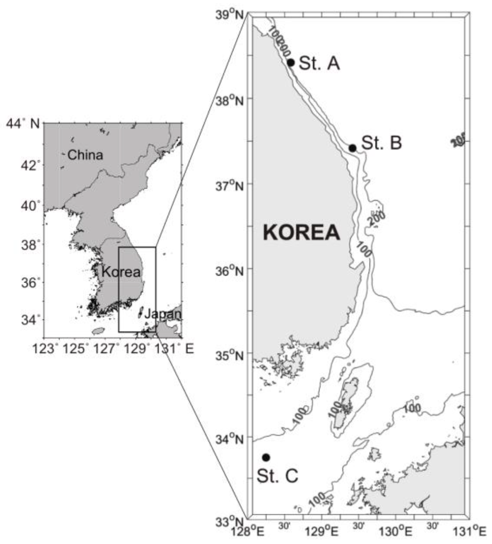
2.1. Study Sites

Sampling was performed at two eastern (St. A and St. B) coastal regions and one southern (St. C) coastal region of the Korean Peninsula (Figure 1) during May (pre-monsoon) and October (post-monsoon) 2020. Each sampling area had low tidal amplitude (less than 30 cm) and water depth ranging from approximately 100 m to 170 m. In the East Sea sampling areas, the vertical structure of the current generally shows a two-layer system with a branch of the TWC (East Korean Warm Current) in the upper layer and a branch of the LCC (North Korean Cold Current) in the deeper layer [28]. Conversely, the South Sea is a region of diverse marine environments with a branch of the TWC flowing through the sampling area into the East Sea [26]. The environmental conditions of the sampling sites are listed in Table 1. During both seasons, the surface layer water temperatures in the South Sea were relatively high (20.3 °C in May and 24.7 °C in October) compared to those in the East Sea (14.9–15.3 °C in May and 16.2–16.5 °C in October). Similarly, the bottom layer water temperature was highest (24.5 °C at St. C) in October and lowest (1.0 °C at St. B) in May. The salinities of the surface water ranged from 32.4 (St. B) to 34.5 (St. A) in May and from 32.6 (St. B) to 33.8 (St. C) in October, while those of the bottom water were relatively constant (34.0 in St. A and B and 34.4 to 34.5 in St. C). Chlorophyll a (Chl a) concentrations of the surface layers varied between 0.7 μg/L (St. B) and 1.4 μg/L (St. A) in May, and between 0.3 μg/L (St. A) and 0.7 μg/L (St. B) in October.

2.2. Sample Collection and Processing

Field surveys were performed on board the R/V Tamgu 22 at the three sites during two cruises in May and October 2020. Temperature and salinity data were obtained using a CTD (SBE 911 Plus, Seabird Electronics Inc., Bellevue, WA, USA). To collect chl a and suspended particulate organic matter (SPOM), seawater samples (approximately 20 L) were collected from the subsurface layers on each sampling occasion. Subsequently, the water samples were pre-filtered through a 200 μm mesh sieve to remove zooplankton and large particles. The pre-filtered samples were re-filtered on pre-combusted (450 °C for 4 h) Whatman GF/F glass fiber filters, using a vacuum pump, which were then frozen in a deep freezer (−20 °C) for later processing. In the laboratory, the chl a from the filter samples was extracted with 90% acetone overnight in darkness and sonicated for 5 min. After the extraction, the Chl a concentrations were determined using a fluorometer (Model 10 AU 005; Turner Designs, San Jose, CA, USA). The filtered samples for stable isotope analysis were acidified by fuming overnight over 1 N HCl to remove inorganic carbonates, oven-dried at 50 °C for 24 h, and then kept frozen at −20 °C until isotope analysis.
Samples of dominant zooplankton groups, copepods, and euphausiids as isotopic base line were collected by obliquely towing a Bongo net (60 cm mouth diameter, 200 and 330 μm mesh), equipped with a flowmeter, at a depth of 100 m [12]. Partial zooplankton samples were preserved in 90% ethanol for taxonomic identification and the remainder were frozen at −20 °C. Following transport to the laboratory, copepods and euphausiids were identified under a dissecting microscope.
All fish specimens were collected using a bottom trawl, which had a 6-seam net constructed of 120 mm (stretched) polyethylene mesh in the main body of the net, an 80 mm mesh in the intermediate part of the net, and a 60 mm mesh in the cod end with a 20 mm cod-end liner. The trawl was spread using a Jet 2 type; it had 5.14 m2 quadrangle doors and weighed 1990 kg. The fishing depth ranges averaged from 107.7 m to 167.1 m. All collected samples were sorted and identified to the species level, then their total lengths and weights were measured to the nearest 0.1 cm and 0.1 g, respectively. For isotope analysis, only the white muscle tissue of fish was used and was separated from the anterior dorsal regions using a knife. Squid and octopus muscle tissues were carefully dissected from the anterior mantle. All animal samples were freeze-dried, pulverized into a fine powder using a ball mill (MM200; Retsch GmbH, Haan, Germany), and then kept frozen (−20 °C) until isotope analysis.

2.3. Stable Isotope Analyses

Powdered zooplankton and fish samples (0.5–1.0 mg) were transferred to tin combustion capsules, and filter samples were wrapped in tin disks. All sealed samples were combusted at 1020 °C in a CNSOH elemental analyzer (EA Isolink, Bremen, Germany) and the resultant gases were analyzed using a linked continuous-flow isotope ratio mass spectrometer (CF-IRMS; DELTA V PLUS, Bremen, Germany). The stable isotope ratios are expressed in δ notation relative to conventional standard reference materials (Vienna Pee Dee Belemnite for carbon and atmospheric N2 for nitrogen), as follows: δ X   ( ) = [ ( R s a m p l e R s t a n d a r d ) 1 ] × 10 3 , where X is 13C or 15N and R is 13C/12C or 15N/14N. To calibrate the system, international standards for sucrose (ANU C12H22O11; NIST, Gaithersburg, MD, USA) and ammonium sulfate ([NH4]2SO4; NIST) were used as reference standards. The analytical precision based on 20 replicates of urea was within 0.15‰ and 0.18‰ for δ13C and δ15N, respectively.
The differences in the lipid content among fish samples can result in bias in the interpretation of their δ13C values [29]. Thus, we used a lipid correction method proposed by [30], in which the mass C:N ratios from the elemental fractions of fish tissues were assessed to determine whether the values were greater than 3.5, which may have indicated potential lipid bias. For C:N ratios greater than 3.5, lipid correction was performed as follows: δ 13 C n o r m a l i z e d = δ 13 C u n t r e a t e d 3.32 + 0.99 × C : N   ( r a t i o s ) , where δ 13 C u n t r e a t e d and δ 13 C n o r m a l i z e d are the measured and lipid-normalized values of the sample, respectively.
The trophic position (TP) of fish was calculated using the equation: T P i = ( δ 15 N i δ 15 N b a s e l i n e ) / Δ 15 N + 2 , where δ15Ni represents the mean δ15N of the fish species, δ15Nbaseline is the mean δ15N of the food-web baseline, δ 15 N is the enrichment factor (3.4‰; [24]) in δ15N per TP, and 2 represents the baseline TP. The mean δ15N value of calanoid copepods at each sampling site was used as the trophic baseline.

2.4. Data Analyses

Prior to statistical analyses, all data were tested for normality and homogeneity of variance using the Shapiro–Wilk procedure and Levene’s test, respectively, using IBM SPSS software (ver. 21.0, IBM Corp., Armonk, NY, USA). One-way analysis of variance (ANOVA), followed by Tukey’s honest significant difference (HSD) multiple comparison post hoc test were used to distinguish significant differences in the δ13C and δ15N values of fish species among sampling sites and seasons. Significant differences in both the isotopic values of SPOM, zooplankton, and fish consumers among sampling sites and seasons were tested using a permutational multivariate analysis of variance (PERMANOVA). A PERMANOVA design was performed on two factors: seasons (fixed with two levels of May and October) and sites (fixed with three levels of Sites A, B, and C). The PERMANOVA test was conducted using PRIMER version 6 (PRIMER-e, Auckland, New Zealand), with the PERMANOVA + PRIMER add-on [31].
Isotopic niche parameters (total area; TA; and sample size-corrected standard ellipse area, SEAc) of fish assemblages were used to compare the trophic structure and trophic diversity among sampling sites and between seasons. This was done using the Stable Isotope Bayesian Ellipses in R (SIBER) package within R software (version 4.1.1; R Core Team). The TA values were assessed by a convex hull area encompassed by the points of all species in a δ13C–δ15N bi-plot space, providing a measure of the total amount of isotopic niche space of consumers [32]. The SEAc values were calculated as a quantification of the isotopic δspace to avoid problems because of small sample sizes [33].

3. Results

3.1. Community Structure of Fish Assemblages

The species number and abundance (individuals/km2) of fish assemblages varied among the three sampling sites and between the two seasons, ranging from 12 (St. B in May) to 47 (St. C in May) and from 8996 (St. A in May) to 61051 (St. A in October), respectively (Table 2 and Supplementary Table S1). At St. A and St. B of the East Sea during the two seasons, Glyptocephalus stelleri and Gadus macrocephalus generally dominated the fish assemblages, accounting for 75% and 71% of all individuals, respectively. In contrast, Dentex tumifrons, Trachurus japonicus, and Zeus faber at St. C of the South Sea were the most dominant species during the two seasons, accounting for 73% of all individuals. Univariate ecological indices of richness (R), evenness (J), and diversity (H′) varied widely among the three sampling sites and between the two seasons, ranging from 1.08 (St. B in May) to 4.72 (St. C in May), 0.44 (St. A in October) to 0.80 (St. A in May), and 1.31 (St. A in October) to 2.12 (St. C in May), respectively (Table 2).

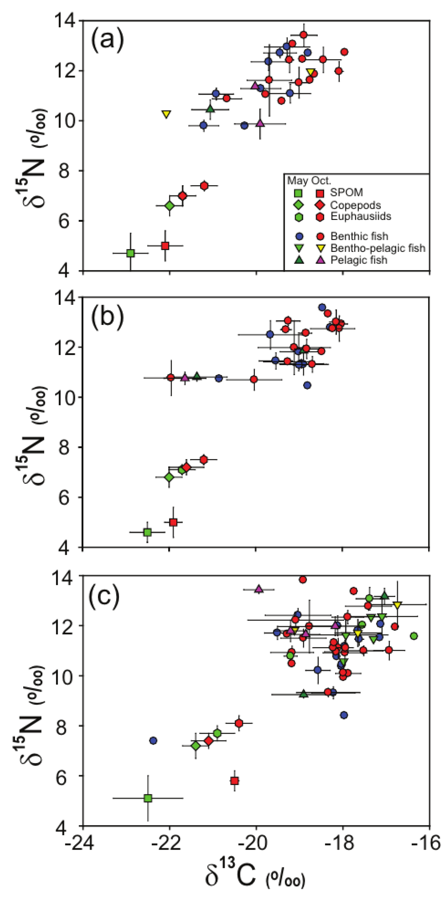
3.2. Stable Isotope Values of SPOM and Zooplankton

The δ13C and δ15N values of SPOM differed significantly among the sampling sites (PERMANOVA, pseudo-F 2, 29 = 7.18, p = 0.004) and between seasons (pseudo-F 1, 29 = 15.70, p = 0.001), ranging from −22.9 ± 0.3‰ (St. A in May) to −20.5 ± 0.1‰ (St. C in October) and from 4.6 ± 0.4‰ (St. B in May) to 5.8 ± 0.3‰ (St. C in October), respectively (Table 3). Similarly, significant differences in the isotopic values of zooplankton (both calanoid copepods and euphausiids) were observed among the sampling sites (pseudo-F 2, 23 = 5.47, p = 0.012; pseudo-F 2, 23 = 15.25, p = 0.001) and between seasons (pseudo-F 1, 23 = 5.42, p = 0.029 and pseudo-F 1, 23 = 14.33, p = 0.001), showing the lowest δ13C at St. A in May and the highest at St. C in October for all cases. These overall mean δ13C and δ15N values varied between −22.0 ± 0.3‰ and −21.1 ± 0.4‰, and between 6.6 ± 0.4‰ to 7.4 ± 0.3‰ for copepods, and between −21.7 ± 0.3‰ and −20.4 ± 0.3‰ from 7.0 ± 0.4‰ to 8.1 ± 0.3‰ for euphausiids, respectively.

3.3. Stable Isotope Values of Fish Assemblages

The δ13C and δ15N values of fish assemblages varied significantly between seasons (pseudo-F 1, 252 = 5.41, p = 0.010) and among sites (pseudo-F 2, 252 = 18.98, p = 0.001), whereas no significant effect of the interaction term of season × site (pseudo-F 2, 252 = 1.57, p = 0.200) (Figure 2 and Table 4 and Table 5) was observed. Additionally, the isotope values for fish consumers at the two sites within the East Sea significantly differed between seasons (pseudo-F 1, 129 = 5.06, p = 0.027) and sites (pseudo-F 1, 129 = 5.46, p = 0.017). No significant effect of the interaction term (site × season; pseudo-F 1, 129 = 1.54, p = 0.196) was found in this case. The overall mean δ13C values of fish consumers in May were significantly different among the three sites (Tukey’s HSD test, F2, 90 = 32.23, p < 0.01; −21.2 ± 0.3‰ to −18.8‰, −21.4 ± 0.7‰ to −18.3‰, and −22.4‰ to −17.0 ± 0.2‰ at St. A, B, and C, respectively). In October, the δ13C values were relatively higher at the C site (−19.9 ± 0.4‰ to −15.3‰) than at St. A and B (Tukey’s HSD test, F2, 161 = 23.91, p < 0.01; −22.1‰ to −18.0‰ and −22.0 ± 0.6‰ compared to −18.0 ± 0.1‰, respectively). Similar ranges of δ15N values were observed among the three sites in May (Tukey’s HSD test, F2, 90 = 1.01, p = 0.371; 9.8 ± 0.1‰ to 12.9 ± 0.4‰, 10.5‰ to 13.6‰, and 7.4‰ to 13.2 ± 0.3‰ at St. A, B, and C, respectively) and October (Tukey’s HSD test, F2, 161 = 0.95, p = 0.389; 9.9 ± 0.6‰ to 13.4 ± 0.4‰, 10.7 ± 0.4‰ to 13.3‰, and 9.3 ± 0.2‰ to 13.8‰ at St. A, B, and C, respectively).

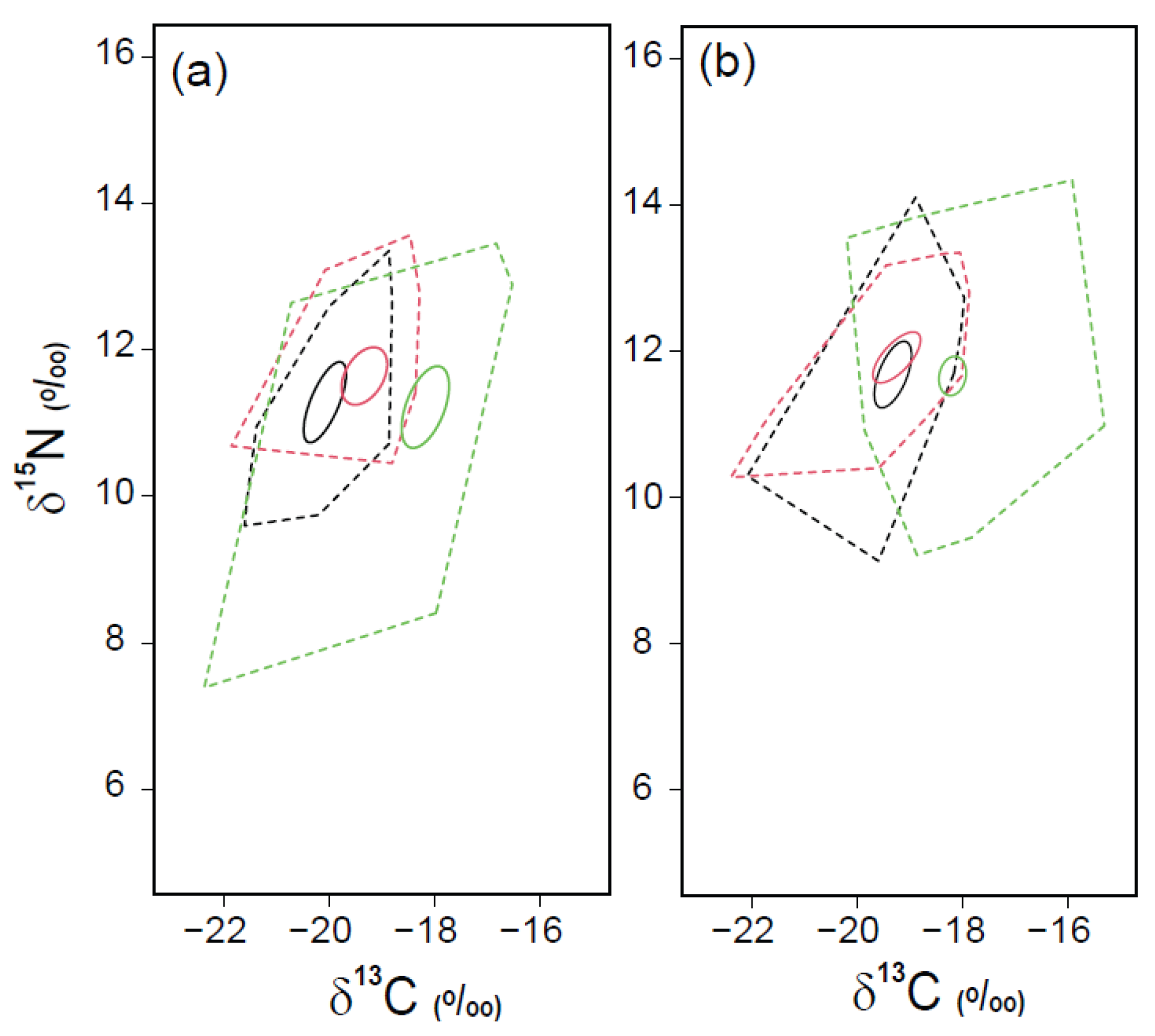
3.4. Trophic Positions and Isotopic Niche Areas of Fish Assemblages

We calculated the TP value of each fish consumer based on the mean δ15N value of calanoid copepods at each site in each season (Table 4 and Table 5). In May, fish consumer TPs differed significantly among the three sites (Tukey’s HSD test, F2, 90 = 4.31, p = 0.016), ranging from 2.94 to 3.87, 3.08 to 3.99, and 2.05 to 3.76 at St. A, B, and C, respectively. In contrast, no significant differences were observed in the TP values among the three sites in October (Tukey’s HSD test, F2, 162 = 1.22, p = 0.297), which ranged from 2.84 to 3.89, 3.03 to 3.80, and 2.63 to 3.95 at St. A, B, and C, respectively.
The isotopic niche areas (‰2) of fish assemblages at the three sites in the two seasons were estimated using the TA and SEAc values (Figure 3). In both seasons, the TA and SEAc values were relatively higher at the St. C (21.20 and 4.53 in May, and 17.92 and 3.03 in October, respectively) compared to those at St. A (6.13 and 2.35 in May, and 9.89 and 2.50 in October, respectively) and St. B (6.99 and 2.12 in May, and 7.54 and 2.56 in October, respectively).

4. Discussion

The present study demonstrated the spatial and temporal variations in the trophic structure of fish assemblages in the East and South Seas of Korea by comparing their carbon and nitrogen stable isotope ratios and species compositions over two seasons. Our major results showed that the isotopic ratios of fish assemblages, with the food-web base and dietary items, were spatially and seasonally variable. This reflects the regional-specific effects of oceanographic and geographical characteristics on the differences in the species composition and trophic structure between the two seas. Particularly, the presence of specific fish consumers due to differences in species composition may lead to spatial and seasonal variations in trophic structure resulting from changes in trophic niche indices. Information on the trophic dynamics of marine ecosystems under different environmental conditions can allow for a deeper understanding of climate-related changes in trophic diversity and community structure.
The fish communities in the East Sea and South Sea are generally known to have considerable differences in species composition and abundance, due to different environmental conditions [26]. In the present study, the total composition and abundance of fish species collected from the sampling sites during the two seasons were similar to those previously reported in the East and South Seas of Korea [34,35,36,37]. In particular, clearly distinct dominant species between the two seas are among the most common characteristics of fisheries resources in Korean coastal waters, as reported in many studies [34,38,39,40]. The relatively high diversity of fish species in the South Sea (47 and 36 species recorded in May and October, respectively) compared to those in the East Sea (12–16 and 19 species recorded in May and October, respectively) may be related to the unique environmental conditions created by complex interactions caused by the TWC input from the south and nutrient-enriched freshwater from major river systems of Seomjin, Nam, and Nakdong River (Moon et al., 2015). Similarly, fish communities in the East Sea are mostly comprised of resident and/or demersal fishes, such as the families Pleuronectidae and Cottidae, suggesting that certain biological characteristics occur only in the eastern coastal waters of the Korean Peninsula rather than in the South Sea [35,39].
Physical environmental changes may result in major temporal differences in the species composition and abundance of fish assemblages. The fish assemblages in the southern and eastern coastal waters of the Korean Peninsula may be substantially impacted by oceanographic conditions (e.g., seawater temperature and the thermal structure of the water mass) due to changes in the Kuroshio Current [27]. In fact, [36] reported that the alteration in the oceanographic boundary of a thermal front could influence fish composition in mid-eastern coastal waters, related to the change in distribution of migratory pelagic species. Furthermore, the differences in seawater temperatures between the two seas may be the main factor causing the distinct species composition and abundance of fish assemblages. Because the range of seawater temperatures can directly or indirectly influence the life cycles (e.g., growth, reproduction, physiology, and behavior) of fish species, their spatial and seasonal variability may control the dynamics in fish communities and geographical inhabiting ranges [41,42]. Thus, the spatial and seasonal variations in the composition and abundance of fish assemblages may be a feature of fish communities in Korean coastal waters, resulting from environmental changes in physical and trophic conditions affected by regional differences.
In the present study, despite the significant differences in the δ13C and δ15N of SPOM, little spatial and seasonal variations in the isotopic values were found in both cases (0.4–1.6‰ and 0.5–0.8‰, respectively). Spatial and seasonal variations in the δ13C and δ15N of SPOM may be influenced by changes in physical/chemical (e.g., water temperature and availability of dissolved inorganic carbon and nitrogen) and biological factors (e.g., phytoplankton taxonomic groups and their growth rates) under ambient environmental conditions [43,44,45]. Nevertheless, the δ13C and δ15N values of SPOM were consistent with previously reported ranges (−24 to −18‰ for δ13C and 2 to 10‰ for δ15N) of general marine phytoplankton in coastal waters of the Korean Peninsula and other temperate regions [12,22,46]. The isotopic results suggest that organic matter derived from phytoplankton may be the most important source of the SPOM pool in both seas. In this respect, despite the statistical isotopic differences for zooplankton, their δ13C and δ15N values showed very similar patterns in spatial and seasonal variability (0.5–0.8‰ and 0.4–0.6 for copepods, and 0.8 and 0.6–0.7 for euphausiids, respectively) with those of SPOM as a food-web baseline. Overall, our results suggest that the temporal isotopic trends of the trophic base line and lower trophic levels showed similar variability among the sampling sites during the two seasons.
Dual isotope plots for all sites in both seasons showed a notable pattern of increasing δ13C and δ15N values of fish species with increasing TPs due to the isotopic enrichment per trophic level. Regardless of sampling site, most fish species showed a continuum of δ13C and δ15N ranges along the TPs from the isotopic points of SPOM and zooplankton, suggesting that the trophic pathways may link phytoplankton-derived organic matter to fish assemblages. Additionally, based on the feeding zones classified by pelagic and benthic life patterns, demersal fishes generally exhibited higher δ13C and δ15N values than pelagic fishes. This result is consistent with those of several previous studies on greater 13C- and 15N-enrichments in benthic pathways than in pelagic pathways, suggesting the differentiation between benthic and pelagic food webs [12,47,48]. Indeed, such enriched ranges for δ13C and δ15N in fish species may be closely associated with the behavioral features of pelagic and benthic feeding strategies, and prey items along the trophic continuum, respectively. In terms of fish species trophic ecology, larger-sized individuals as predators or piscivores may generally tend to feed on large prey items, and thus are at the top of the δ13C–15N dual isotope plot. In contrast, smaller fish species may feed mostly on invertebrates as preferred prey items compared to other fish individuals, reflecting their lower δ15N values. This size-dependent feeding pattern related to fish ecology of the present study is likely responsible for the position of fish species in the dual isotope plot, which reflects a general isotopic trend in common marine fish [47,49].
Most fish species have a common characteristic of opportunistic feeding behavior, which is mainly influenced by ambient food availability [50]. In this regard, the spatial and seasonal patterns in the trophic structure of fish assemblages may be closely associated with the status of environmental conditions, which may lead to a dynamic utilization of available resources and diversity of prey items [51]. Furthermore, the specific food-web structure may be organized by a variety of trophic pathways involving many component species within the community. Above all, because pelagic and migrating fish species may respond sensitively to ambient environmental conditions, the dynamics of pelagic trophic structures in coastal ecosystems can be clearly influenced by spatial and seasonal changes in species composition [12]. Therefore, the principal distinctions in the trophic structures of fish assemblages between the East Sea and the South Sea may be mainly induced by the differences in environmental factors, implying distinct prey availability for fish associated with the different oceanographic conditions discussed above.
Spatial and seasonal variability in the ecological and trophic niches of consumer species have been investigated using the isotopic niche parameters of TA and SEAc, allowing for the identification of intra- and interspecific competition for prey items, and spatiotemporal shifts in food-web structure [12,32,52]. The ranges of isotopic niche areas are important for estimating the diversity of trophic pathways within a complicated ecosystem [52]. In our study, during both seasons, the TA and SEAc of fish assemblages in the South Sea exhibited wider ranges than those in the East Sea. Such spatial differences in the isotopic niche areas may mostly result from the different environmental conditions and/or species compositions that can alter the trophic relationships within the community [53,54]. Our results also suggest that the spatial differences in the TA and SEAc may be associated with the regional distinction in the fish community interacting with different environmental conditions. In general, regional environmental differences, due to longitudinal and latitudinal changes in physical and chemical factors, are likely to alter the community components from low trophic organisms to top predators, and may therefore reflect the regional isotopic variation in the different prey–consumer relationships [54,55]. As a result, the site differences in the isotopic niche parameters are likely due to differences in the species composition of fish assemblages adapting to ambient environmental conditions with different levels of food availability.
In conclusion, our isotopic investigation of fish assemblages showed spatial differences in the food-web structure and species composition between the East and South Seas of the Korean Peninsula, implying the occurrence of different environmental conditions. Additionally, the isotopic niche indices were relatively higher in the South Sea compared to those in the East Sea, suggesting the distinction of trophic diversity of fish assemblages, coupled with the relative differences in abundance and population size of component species. Overall, our isotopic evidence implies that spatial and temporal variations in fish communities in response to changing environmental conditions (especially changing of major currents and ocean warming) can alter the trophic relationships among species and the food-web structure. Further long-term studies considering top-down and bottom-up trophic processes, based on community compositions of fish assemblages and their stable isotope ratios, are needed to better understand the functioning of coastal ecosystems under global climate change.

Supplementary Materials

The following supporting information can be downloaded at: https://www.mdpi.com/article/10.3390/w14010058/s1, Table S1: Abundance (Individuals/km2) and biomass (kg/km2) of fish assemblages collected at the St. A, St. B, and St. C during May and October 2020.

Author Contributions

D.S. and H.J.P. designed the experiments and drafted the manuscript; D.S., K.H., D.N.K., S.-J.L., and S.K. designed field collection and analyzed faunal assemblages; T.H.P. and C.-I.L. performed the statistical analyses; D.S. and H.J.P. wrote the main manuscript text; H.J.P. supervised all processes; All authors analyzed the data and reviewed the manuscript. All authors have read and agreed to the published version of the manuscript.

Funding

This research was supported by the National Institute of Fisheries Science, Korea (R2021027) and the National Research Foundation of Korea (NRF- 2021R1A2C1012537), Ministry of Science and ICT, Korea.

Data Availability Statement

The data presented in this study are available on request from the corresponding author.

Acknowledgments

We would like to thank the captain and crews of the R/V Tamgu 22 for field observation and sampling of fish assemblages.

Conflicts of Interest

The authors declare no conflict of interest.

References

  1. McLusky, D.S.; Elliott, M. The Estuarine Ecosystem: Ecology Threats and Management; Oxford University Press: New York, NY, USA, 2004; p. 214. [Google Scholar]
  2. Akin, S.; Winemiller, K.O.; Gelwick, F.P. Seasonal and spatial variations in fish and macrocrustacean assemblage structure in Mad Island Marsh estuary, Texas. Estuar. Coast. Shelf Sci. 2003, 57, 269–282. [Google Scholar] [CrossRef]
  3. Costanza, R.; d’Arge, R.; de Groot, R.; Farber, S.; Grasso, M.; Hannon, B.; Naeem, S.; Limburg, K.; Paruelo, J.; O’Neill, R.V.; et al. The value of the world’s ecosystem services and natural capital. Nature 1997, 387, 253–260. [Google Scholar] [CrossRef]
  4. Dunson, W.A.; Travis, J. The role of abiotic factors in community organization. Am. Nat. 1991, 138, 1067–1091. [Google Scholar] [CrossRef]
  5. Thompson, R.M.; Brose, U.; Dunne, J.A.; Hall, R.O., Jr.; Hladyz, S.; Kitching, R.L.; Martinez, N.D.; Rantala, H.; Romanuk, T.N.; Stouffer, D.B.; et al. Food webs: Reconciling the structure and function of biodiversity. Trends Ecol. Evol. 2012, 27, 689–697. [Google Scholar] [CrossRef] [Green Version]
  6. McMeans, B.C.; McCann, K.S.; Humphries, M.; Rooney, N.; Fisk, A.T. Food web structure in temporally-forced ecosystems. Trends Ecol. Evol. 2015, 30, 662–672. [Google Scholar] [CrossRef] [PubMed]
  7. Willis, T.V.; Wilson, K.A.; Johnson, B.J. Diets and stable isotope derived food web structure of fishes from the inshore Gulf of Maine. Estuar. Coast. 2017, 40, 889–904. [Google Scholar] [CrossRef]
  8. Johnson, C.R.; Seinen, I. Selection for restraint in competitive ability in spatial competition systems. Proc. R. Soc. Lond. B Biol. Sci. 2002, 269, 655–663. [Google Scholar] [CrossRef] [PubMed] [Green Version]
  9. Timmerman, C.-A.; Giraldo, C.; Cresson, P.; Ernande, B.; Travers-Trolet, M.; Rouquette, M.; Denamiel, M.; Lefebvre, S. Plasticity of trophic interactions in fish assemblages results in temporal stability of benthic-pelagic couplings. Mar. Environ. Res. 2021, 170, 105412. [Google Scholar] [CrossRef]
  10. Garrison, L.P.; Link, J.S. Dietary guild structure of the fish community in the Northeast United States continental shelf ecosystem. Mar. Ecol. Prog. Ser. 2000, 202, 231–240. [Google Scholar] [CrossRef]
  11. Pace, M.L.; Cole, J.J.; Carpenter, S.R.; Kitchell, J.F. Trophic cascades revealed in diverse ecosystems. Trends Ecol. Evol. 1999, 14, 483–488. [Google Scholar] [CrossRef]
  12. Park, T.H.; Lee, C.I.; Kang, C.K.; Kwak, J.H.; Lee, S.H.; Park, H.J. Seasonal variation in food web structure and fish community composition in the East/Japan sea. Estuar. Coast. 2020, 43, 615–629. [Google Scholar] [CrossRef]
  13. Pasquaud, S.; Elie, P.; Jeantet, C.; Billy, I.; Martinez, P.; Girardin, M. A preliminary investigation of the fish food web in the Gironde estuary France, using dietary and stable isotope analyses. Estuar. Coast. Shelf Sci. 2008, 78, 267–279. [Google Scholar] [CrossRef]
  14. Last, P.R.; White, W.T.; Gledhill, D.C.; Hobday, A.J.; Brown, R.; Edgar, G.J.; Pecl, G. Long-term shifts in abundance and distribution of a temperate fish fauna: A response to climate change and fishing practices. Glob. Ecol. Biogeogr. 2011, 20, 58–72. [Google Scholar] [CrossRef]
  15. Cury, P.; Shin, Y.J.; Planque, B.; Durant, J.; Fromentin, J.M.; Kramer-Schadt, S.; Stenseth, N.; Travers, M.; Grimm, V. Ecosystem oceanography for global change in fisheries. Trends Ecol. Evol. 2008, 23, 338–346. [Google Scholar] [CrossRef]
  16. Baker, R.; Fujiwara, M.; Minello, T.J. Juvenile growth and mortality effects on white shrimp Litopenaeus setiferus population dynamics in the northern Gulf of Mexico. Fish. Res. 2014, 155, 74–82. [Google Scholar] [CrossRef]
  17. Hertz, E.; Robinson, J.P.; Trudel, M.; Mazumder, A.; Baum, J.K. Estimation of predator-prey mass ratios using stable isotopes: Sources of errors. Mar. Ecol. Prog. Ser. 2014, 516, 1–6. [Google Scholar] [CrossRef] [Green Version]
  18. Michener, R.H.; Schell, D.M. Stable isotope ratios as tracers in marine aquatic food webs. In Stable Isotopes in Ecology and Environmental Science; Lajtha, K., Michener, R.H., Eds.; Blackwell Scientific: Oxford, UK, 1994; pp. 138–157. [Google Scholar]
  19. Boecklen, W.J.; Yarnes, C.T.; Cook, B.A.; James, A.C. On the use of stable isotopes in trophic ecology. Annu. Rev. Ecol. Syst. 2011, 42, 411–440. [Google Scholar] [CrossRef] [Green Version]
  20. Layman, C.A.; Araujo, M.S.; Boucek, R.; Hammerschlag-Peyer, C.M.; Harrison, E.; Jud, Z.R.; Post, D.M. Applying stable isotopes to examine food-web structure: An overview of analytical tools. Biol. Rev. 2012, 87, 545–562. [Google Scholar] [CrossRef]
  21. DeNiro, M.J.; Epstein, S. Influence of diet on the distribution of carbon isotopes in animals. Geochim. Cosmochim. Acta 1978, 42, 495–506. [Google Scholar] [CrossRef]
  22. Fry, B.; Sherr, E.B. δ13C measurements as indicators of carbon flow in marine and freshwater ecosystems. Contrib. Mar. Sci. 1984, 27, 13–47. [Google Scholar]
  23. Vander Zanden, M.J.; Rasmussen, J.B. Variation in 15N and 13C trophic fractionation: Implications for aquatic food web studies. Limnol. Oceanogr. 2001, 46, 2061–2066. [Google Scholar] [CrossRef]
  24. Post, D.M. Using stable isotopes to estimate trophic position: Models, methods, and assumptions. Ecology 2002, 83, 703–718. [Google Scholar] [CrossRef]
  25. Peterson, B.J.; Fry, B. Stable isotopes in ecosystem studies. Annu. Rev. Ecol. Syst. 1987, 18, 293–320. [Google Scholar] [CrossRef]
  26. Jung, H.K.; Rahman, S.M.; Kang, C.-K.; Park, S.-Y.; Lee, S.H.; Park, H.J.; Kim, H.-W.; Lee, C.I. The influence of climate regime shifts on the marine environment and ecosystems in the East Asian Marginal Seas and their mechanisms. Deep. Res. Part II Top. Stud. Oceanogr. 2017, 143, 110–120. [Google Scholar] [CrossRef]
  27. Tian, Y.; Kidokoro, H.; Watanabe, T. Long-term changes in the fish community structure from the Tsushima warm current region of the Japan/East Sea with an emphasis on the impacts of fishing and climate regime shift over the last four decades. Prog. Oceanogr. 2006, 68, 217–237. [Google Scholar] [CrossRef]
  28. Lee, J.C. Water mass distribution and currents in the vicinity of the Hupo Bank in summer 2010. Korean J. Fish. Aquat. Sci. 2016, 49, 61–73. [Google Scholar]
  29. Sweeting, C.J.; Polunin, N.V.C.; Jennings, S. Effects of chemical lipid extraction and arithmetic lipid correction on stable isotope ratios of fish tissues. Rapid Commun. Mass Spectrom. 2006, 20, 595–601. [Google Scholar] [CrossRef]
  30. Post, D.M.; Layman, C.A.; Arrington, D.A.; Takimoto, G.; Quattrochi, J.; Montaña, C.G. Getting to the fat of the matter: Models, methods and assumptions for dealing with lipids in stable isotope analyses. Oecologia 2007, 152, 179–189. [Google Scholar] [CrossRef]
  31. Anderson, M.J.; Clarke, K.R.; Gorley, R.N. PERMANOVA+ for Primer: Guide to Software and Statistical Methods; University of Auckland and PRIMER-E Ltd.: Plymouth, UK, 2008. [Google Scholar]
  32. Layman, C.A.; Arrington, D.A.; Montaña, C.G.; Post, D.M. Can stable isotope ratios provide for community-wide measures of trophic structure? Ecology 2007, 88, 42–48. [Google Scholar] [CrossRef]
  33. Jackson, A.L.; Inger, R.; Parnell, A.C.; Bearhop, S. Comparing isotopic niche widths among and within communities: SIBER–Stable Isotope Bayesian Ellipses in R. J. Anim. Ecol. 2011, 80, 595–602. [Google Scholar] [CrossRef]
  34. Han, K.H. Fish fauna in the south sea of Korea. In Current and Preservarion of Korean Fishes; Ichthyol Soc Korea Symp: Seoul, Korea, 2003; pp. 37–76. [Google Scholar]
  35. Choi, K.H.; Han, M.H.; Kang, C.K.; Park, J.M.; Choi, J.H.; Park, J.H.; Lee, C.I. Seasonal variations in species composition of fish assemblage collected by trammel net in coastal waters of the East Sea. J. Korean Soc. Fish. Ocean. Technol. 2012, 48, 415–427. [Google Scholar] [CrossRef] [Green Version]
  36. Kang, J.H.; Kim, Y.G.; Park, J.Y.; Kim, J.K.; Ryu, J.H.; Kang, C.B.; Park, J.H. Comparison of Fish Species Composition Collected by Set Net at Hupo in Gyeong-Sang-Buk-Do, and Jangho in Gang-Won-Do, Korea. Korean J. Fish. Aquat. Sci. 2014, 47, 424–430. [Google Scholar]
  37. Moon, D.Y.; Jeong, H.G.; Myoung, J.-G.; Choi, J.H.; Kwun, H.J.; Back, J.W.; Hong, S.Y.; Kim, S.Y. Fish Species Collected by the Fish Collection Project from the Southern Sea of Korea during 2010–2012. Korean J. Fish. Aquat. Sci. 2015, 48, 507–528. [Google Scholar]
  38. Lee, T.W. Seasonal variation in species composition of demersal fish in the coastal water off Uljin and Hupo in the East Sea of Korea in 2002. Korean J. Ichthyol. 2011, 23, 187–197. [Google Scholar]
  39. Sohn, M.H.; Park, J.H.; Yoon, B.S.; Choi, Y.M.; Kim, J.K. Species composition and community structure of demersal fish caught by a danish seine fishery in the coastal waters of the middle and southern East Sea, Korea. Korean J. Fish. Aquat. Sci. 2015, 48, 529–541. [Google Scholar]
  40. Song, S.H.; Jeong, J.M.; Lee, S.H.; Kim, D.H. Species composition and community structure of fish by shrimp beam trawl between Sacheon Bay and coastal waters off Namhae, Korea. J. Korean Soc. Fish. Technol. 2019, 55, 217–232. [Google Scholar] [CrossRef]
  41. Stephens, J.S.; Hose, J.E.; Love, M.S. Fish assemblages as indicators of environmental change in nearshore environments. In Marine Organisms as Indicators; Springer: New York, NY, USA, 1988. [Google Scholar]
  42. Pankhurst, N.W.; Munday, P.L. Effects of climate change on fish reproduction and early life history stages. Mar. Freshw. Res. 2011, 62, 1015–1026. [Google Scholar] [CrossRef] [Green Version]
  43. Cifuentes, L.A.; Sharp, J.H.; Fogel, M.L. Stable carbon and nitrogen isotope biogeochemistry in the Delaware Estuary. Limnol. Oceanogr. 1988, 33, 1102–1115. [Google Scholar] [CrossRef]
  44. Goering, J.; Alexander, B.; Haubenstock, N. Seasonal variability of stable carbon and nitrogen isotope ratios of organisms in a N. Pacific bay. Estuar. Coast Shelf. Sci. 1990, 30, 239–260. [Google Scholar] [CrossRef]
  45. Fry, B. 13C/12C fractionation by marine diatoms. Mar. Ecol. Prog. Ser. 1996, 134, 283–294. [Google Scholar] [CrossRef] [Green Version]
  46. Kang, C.K.; Choy, E.J.; Hur, Y.B.; Myeong, J.I. Isotopic evidence of particle size-dependent food partitioning in cocultured sea squirt Halocynthia roretzi and Pacific oyster Crassostrea gigas. Aquat. Biol. 2009, 6, 289–302. [Google Scholar] [CrossRef] [Green Version]
  47. Davenport, S.R.; Bax, N.J. A trophic study of a marine ecosystem off southeastern Australia using stable isotopes of carbon and nitrogen. Can. J. Fish. Aquat. Sci. 2002, 59, 514–530. [Google Scholar] [CrossRef]
  48. Boyle, M.D.; Ebert, D.A.; Cailliet, G.M. Stable isotope analysis of a deep-sea benthic-fish assemblage: Evidence of an enriched benthic food web. J. Fish Biol. 2012, 80, 1485–1507. [Google Scholar] [CrossRef] [PubMed]
  49. Galván, D.E.; Sweeting, C.J.; Reid, W.D.K. Power of stable isotope techniques to detect size-based feeding in marine fishes. Mar. Ecol. Prog. Ser. 2010, 407, 271–278. [Google Scholar] [CrossRef] [Green Version]
  50. Elliott, M.; Whitfield, A.K.; Potter, I.C.; Blaber, S.J.; Cyrus, D.P.; Nordlie, F.G.; Harrison, T.D. The guild approach to categorizing estuarine fish assemblages: A global review. Fish Fish. 2007, 8, 241–268. [Google Scholar] [CrossRef]
  51. Gay, M.; Bao, M.; MacKenzie, K.; Pascual, S.; Buchmann, K.; Bourgau, O.; Levsen, A. Infection levels and species diversity of ascaridoid nematodes in Atlantic cod, Gadus morhua, are correlated with geographic area and fish size. Fish. Res. 2017, 202, 90–102. [Google Scholar] [CrossRef]
  52. Rigolet, C.; Thiébaut, É.; Brind’Amour, A.; Dubois, S.F. Investigating isotopic functional indices to reveal changes in the structure and functioning of benthic communities. Funct. Ecol. 2015, 29, 1350–1360. [Google Scholar] [CrossRef] [Green Version]
  53. Cherel, Y.; Hobson, K.A.; Guinet, C.; Vanpe, C. Stable isotopes document seasonal changes in trophic niches and winter foraging individual specialization in diving predators from the Southern Ocean. J. Anim. Ecol. 2007, 76, 826–836. [Google Scholar] [CrossRef] [PubMed]
  54. Włodarska-Kowalczuk, M.; Aune, M.; Michel, L.N.; Zaborska, A.; Legeżyńska, J. Is the trophic diversity of marine benthic consumers decoupled from taxonomic and functional trait diversity? Isotopic niches of Arctic communities. Limnol. Oceanogr. 2019, 64, 2140–2151. [Google Scholar] [CrossRef] [Green Version]
  55. Kingsbury, K.M.; Gillanders, B.M.; Booth, D.J.; Nagelkerken, I. Trophic niche segregation allows range-extending coral reef fishes to co-exist with temperate species under climate change. Glob. Chang. Biol. 2020, 26, 721–733. [Google Scholar] [CrossRef] [PubMed]
Figure 1. Map of the sampling area in the East Sea (St. A and St. B) and the South Sea (St. C). Field circles indicate the sampling site collected for suspended particulate organic matter (SPOM) and consumers (zooplankton and fish).
Water 14 00058 g001
Figure 2. Dual isotope plots of δ13C and δ15N values of zooplankton and fish consumers and their potential food sources (suspended particulate organic matter, SPOM) at the sampling sites ((a), St. A; (b), St. B; (c), St. C) in May and October. Values are presented as mean δ13C and δ15N (‰ ± 1 SD).
Water 14 00058 g002
Figure 3. The isotopic niche areas (‰2) of fish assemblages collected at the sampling sites (black lines, St. A; red lines, St. B; green lines, St. C) in May (a) and October (b) estimated as total area (TA, dotted line) and standard ellipse area (SEAc, solid line).
Water 14 00058 g003
Table 1. The surface and bottom environmental conditions (water temperature, salinity, and chlorophyll a) in the East Sea (St. A and St. B) and the South Sea (St. C) of Korea during May and October 2020.
MonthWater Temperature (°C)SalinityChl a (µg/L)
SurfaceBottomSurfaceBottomSurface
MayOctoberMayOctoberMayOctoberMayOctoberMayOctober
St. A15.316.23.015.734.532.734.034.01.40.3
St. B14.916.51.016.632.432.634.034.00.70.7
St. C20.324.714.824.533.933.834.534.41.00.6
Table 2. The species number and abundance (individuals/km2) and univariate ecological indices (richness, R; evenness, J; diversity, H′) of fish assemblages collected at the St. A, St. B, and St. C during May and October 2020.
Species NameMay October
St. ASt. BSt. CSt. ASt. BSt. C
Total species number161247191936
Total individuals899527,90617,06761,05313,71540,800
Richness (R)1.651.084.721.631.893.30
Evenness (J)0.800.560.700.440.570.45
Diversity (H′)2.211.402.691.311.671.62
Table 3. δ13C and δ15N values of organic matter (SPOM, suspended particulate organic matter) and zooplankton (calanoid copepods and euphausiids) collected during May and October 2020 in the East Sea (St. A and St. B) and the South Sea (St. C). PERMANOVA test of δ13C and δ15N values for each potential food source between seasons and among sampling sites. Bold-face font indicates significance at p < 0.05. Data represent mean ± 1 SD.
Potential Food Source May October
δ13C δ15N δ13C δ15N
nMeanSDMeanSDnMeanSDMeanSD
St. A
SPOM5−22.90.44.70.85−22.10.45.00.6
Copepods4−22.00.36.60.44−21.70.37.00.4
Euphausiids4−21.70.37.00.44−21.20.37.40.2
St. B
SPOM5−22.50.44.60.45−21.90.25.00.6
Copepods4−22.00.36.80.44−21.60.47.20.3
Euphausiids4−21.70.37.10.24−21.20.37.50.2
St. C
SPOM5−22.50.85.10.95−20.50.15.80.4
Copepods4−21.40.37.20.54−21.10.47.40.3
Euphausiids4−20.90.47.70.34−20.40.38.10.3
PERMANOVA testSeasonSiteInteraction
pseudo-Fppseudo-Fppseudo-Fp
SPOM15.700.0017.180.0041.310.311
Copepods5.420.0295.470.0120.210.896
Euphausiids14.320.00115.250.001Negative
Table 4. δ13C and δ15N values and trophic position (TP) of fish consumers collected at the St. A, St. B, and St. C during May 2020. Lower case codes indicate feeding modes (b, benthic feeder; bp, benthopelagic feeder; p, pelagic feeder). The lipid-correction was applied for the δ13C of marked species (*). Data represent mean ± 1 SD.
Species NameSt. ASt. BSt. C
nδ13Cδ15NTPnδ13Cδ15NTPnδ13Cδ15NTP
MeanS.D.MeanS.D.MeanS.D.MeanS.D.MeanS.D.MeanS.D.
Fish
Ammodytes personatus (b)3 −20.3 0.1 9.8 0.0 2.9
Anisarchus macrops (b) 2 −19.5 0.4 11.4 0.3 3.4
Arctoscopus japonicus (b) 1 −20.8 10.7 3.2
Banjos banjos (b) 1 −17.1 11.5 3.3
Caragoides equula (b) 3 −19.5 0.3 11.7 0.3 3.3
Chelidoperca hirundinacea (b) 1 −18.0 10.4 2.9
Clupea pallasii (p) *3 −21.1 0.4 10.4 0.4 3.1
Coelorhynchus longissimus (bp) 1 −18.0 10.6 3.0
Conger myriaster (b) * 3 −19.0 0.8 12.4 0.3 3.5
Dasycottus setiger (b) 3 −19.0 0.4 11.8 0.8 3.5
Foetorepus altivelis (b) 1 −18.0 8.4 2.4
Gadus macrocephalus (b)2 −19.7 0.4 12.4 0.3 3.7 4 −19.7 0.7 12.5 0.6 3.7
Glyptocephalus stelleri (b) 3 −19.2 0.5 11.1 0.4 3.3 3 −18.9 0.5 11.3 0.2 3.3
Halieutaea stellata (b) 1 −17.1 12.1 3.4
Hemilepidotus gilberti (b)1 −18.8 12.7 3.8 1 −18.5 13.6 4.0
Hemitripterus villosus (b)3 −19.4 0.4 12.7 0.2 3.8
Hippoglossoides dubius (b)3 −19.9 0.5 11.3 0.1 3.4 3 −18.9 0.5 11.3 0.4 3.3
Hoplichthys giberti (b) 2 −18.2 0.5 9.3 0.2 2.6
Icelus cataphractus (b) 3 −19.0 0.1 11.3 0.2 3.3
Laeops kitaharae (b) 1 −22.4 7.4 2.1
Lepidotrigla microptera (b) 1 −18.0 11.2 3.2
Limanda schrencki (b) 1 −18.0 10.5 3.0
Malakichthys wakiyae (p) 3 −18.9 0.7 9.2 0.1 2.6
Pagrus major (b) 2 −18.1 0.1 12.0 0.4 3.4
Pampus argenteus (bp) 1 −17.3 11.5 3.3
Plectranthias kelloggi azumanus (b) 1 −18.1 10.8 3.0
Pleurogrammus azonus (b) *3 −21.2 0.3 9.8 0.2 2.9
Podothecus thompsoni (b) 1 −18.3 12.8 3.8
Psenopsis anomala (bp) 2 −17.9 1.0 11.6 0.8 3.3
Pseudorhombus cinnamoneus (b) 3 −18.6 0.3 10.2 0.5 2.9
Pseudorhombus pentophthalmus (b) 2 −17.6 0.1 11.5 0.2 3.3
Scorpaenodes littoralis (b) 1 −17.7 11.8 3.4
Sebastes owstoni (b) *3 −20.9 0.4 11.1 0.2 3.3 1 −18.8 10.5 3.1
Sphyraena pinguis (p) 4 −17.0 0.2 13.2 0.3 3.8
Taurocottus bergi (b)3 −19.3 0.5 12.9 0.4 3.9
Zenopsis nebulosa (bp) 2 −17.1 0.8 12.4 0.7 3.5
Zeus faber (bp) 2 −17.4 0.4 12.4 0.1 3.5
Cephalopod
Euprymna morsei (bp) 1 −18.9 11.9 3.5
Watasenia scintillans (p) 2 −21.4 0.7 10.8 0.2 3.2
Table 5. δ13C and δ15N values and trophic position (TP) of fish consumers collected at the St. A, St. B, and St. C during October 2020. Lower case codes indicate feeding modes (b, benthic feeder; bp, benthopelagic feeder; p, pelagic feeder). The lipid-correction was applied for the δ13C of marked species (*). Data represent mean ± 1 SD.
Species NameSt. ASt. BSt. C
nδ13Cδ15NTPnδ13Cδ15NTPnδ13Cδ15NTP
MeanS.D.MeanS.D.MeanS.D.MeanS.D.MeanS.D.MeanS.D.
Fish
Allolepis hollandi (b) 2 −18.8 0.1 12.6 0.0 3.6
Anoplagonus occidentalis (b)1 −19.8 11.1 3.2
Argentina kagoshimae (b) 6 −18.9 0.5 11.5 0.4 3.3
Ascoldia variegata (b)2 −18.9 0.3 13.4 0.4 3.9
Aulopus japonicus (b) 2 −18.2 0.3 11.0 0.0 3.1
Beringraja pulchra (b) 1 −16.4 11.6 3.3
Caragoides equula (b) 4 −18.8 0.7 12.0 1.0 3.4
Chelidonichthys spinosus (b) 1 −15.3 11.0 3.1
Chelidoperca hirundinacea (b) 2 −18.1 0.0 11.1 0.4 3.2
Clupea pallasii (p) *1 −20.0 11.4 3.3 4 −21.6 0.5 10.8 0.3 3.0
Conger myriaster (b) * 2 −19.1 1.1 12.2 0.3 3.5
Cookeolus japonicus (b) 1 −19.2 10.5 3.0
Cottiusculus gonez (b)1 −19.4 10.8 3.1 2 −19.3 0.6 11.4 0.0 3.2
Dentex tumifrons (b) 6 −17.9 0.4 12.3 0.3 3.5
Echelus uropterus (b) 1 −16.8 11.9 3.4
Enophrys diceraus (b)1−18.0 12.7 3.7
Eopsetta grigorjewi (b) 2 −17.5 0.4 11.0 0.2 3.1
Foetorepus altivelis (b) 2 −18.3 0.7 9.3 0.2 2.6
Gadus macrocephalus (b)5 −19.7 0.5 11.6 1.4 3.4 5 −19.1 0.8 12.0 1.1 3.4
Gymnocanthus herzensteini (b) *2 −18.1 0.1 12.0 0.4 3.5 2 −18.1 12.7 0.5 3.6
Hippoglossoides dubius (b) 6 −18.7 0.4 11.3 0.3 3.2
Hoplichthys giberti (b) 2 −17.9 0.3 10.1 0.0 2.8
Hoplobrotula armata (b) 1 −17.5 12.0 3.4
Hypsagonus quadricornis (b)1 −18.9 12.5 3.6
Icelus cataphractus (b) 6 −18.8 0.3 11.9 0.4 3.4
Leiognathus nuchalis (b) 2 −19.9 0.3 13.4 0.2 3.8
Lepidotrigla microptera (b) 4 −18.2 0.5 11.1 0.2 3.2
Leptagonus leptorhynchus (b)3 −18.5 0.4 12.4 0.5 3.6 2 −18.0 0.1 12.9 0.0 3.7
Liparis tessellatus (b) 2 −20.0 0.6 10.7 0.4 3.0
Lophius litulon (b) 4−17.40.512.80.23.6
Lycodes nakamurae (b) 2 −19.3 0.1 12.7 0.1 3.6
Maurolicus muelleri (b) 2 −22.0 0.6 10.8 0.7 3.0
Monocentris japonica (b) 1 −17.7 13.4 3.8
Petroschmidtia toyamensis (b) 2 −18.2 0.5 12.7 0.1 3.6
Plectranthias kelloggi azumanus (b) 1−18.0 9.9 2.8
Podothecus thompsoni (b)4 −19.2 0.1 12.4 0.5 3.6 2 −18.1 0.1 13.0 0.5 3.7
Psenopsis anomala (b) 1 −19.1 11.8 3.4
Repomucenus ornatipinnis (b) 1 −17.9 11.1 3.1
Saurida undosquamis (b) 1 −18.9 13.8 3.9
Sebastes owstoni (b) *2 −20.7 0.3 10.9 0.1 3.1
Sebastiscus marmoratus (b) 2 −16.9 0.4 11.0 0.4 3.1
Stichaeus grigorjewi (b) 2 −19.2 0.3 13.0 0.2 3.7
Synagrops philippinensis (b) 4 −19.2 0.5 10.9 0.3 3.1
Synodus macrops (b) 2 −18.2 0.1 11.3 0.0 3.2
Taurocottus bergi (bp)1 −19.2 13.1 3.8 1 −18.3 13.3 3.8
Thamnaconus modestus (b) 2 −17.4 0.3 13.1 0.5 3.7
Trachurus japonicus (p) * 4 −19.2 0.4 11.8 0.4 3.4
Triglops jordani (b)1 −18.7 11.9 3.4 1 −18.5 11.8 3.4
Upeneus japonicus (b) 3 −18.4 0.9 11.2 0.6 3.2
Zenopsis nebulosa (bp) 2 −17.7 0.5 11.7 0.5 3.3
Zeus faber (bp) 6 −16.7 0.7 12.8 0.9 3.7
Cephalopod
Berryteuthis magister (bp)1 −22.1 10.3 3.0
Enteroctopus dofleini (b) *4 −19.0 0.2 11.5 0.6 3.3
Euprymna morsei (bp)1 −18.7 12.0 3.5
Loligo bleekeri (p) 3 −19.2 0.2 10.8 0.1 3.1
Loligo beka (p) 4 −18.2 0.7 12.0 0.4 3.4
Loligo japonica (p) 2 −18.9 0.3 11.6 0.1 3.3
Octopus longispadiceus (b)1 −18.8 11.6 3.4
Sepia esculenta (b) 2 −18.0 0.0 10.1 0.1 2.9
Todarodes pacificus (p)4 −19.9 0.6 9.9 0.6 2.8
Publisher’s Note: MDPI stays neutral with regard to jurisdictional claims in published maps and institutional affiliations.

