Evaluation of CYGNSS Observations for Flood Detection and Mapping during Sistan and Baluchestan Torrential Rain in 2020


Abstract
1. Introduction
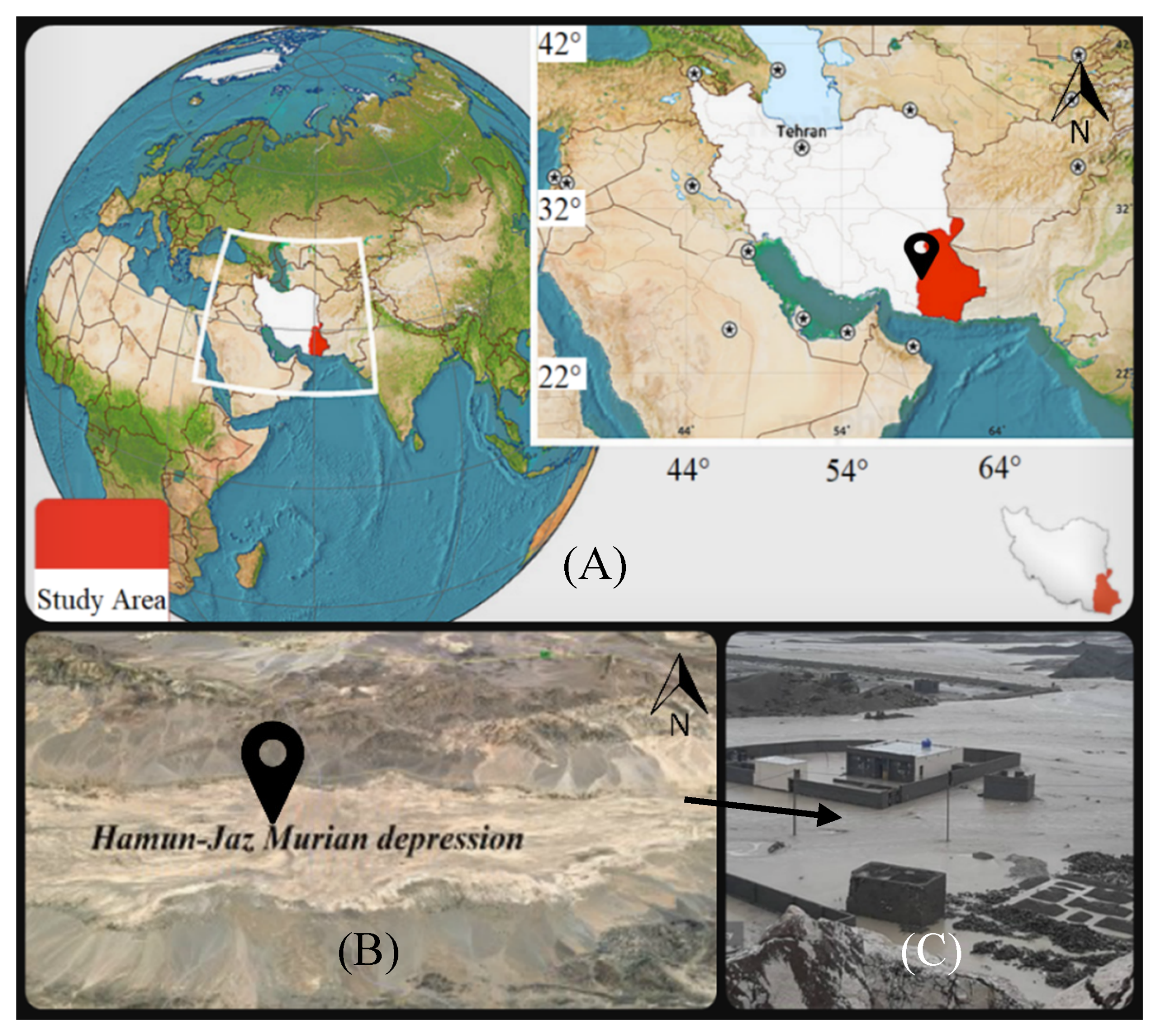
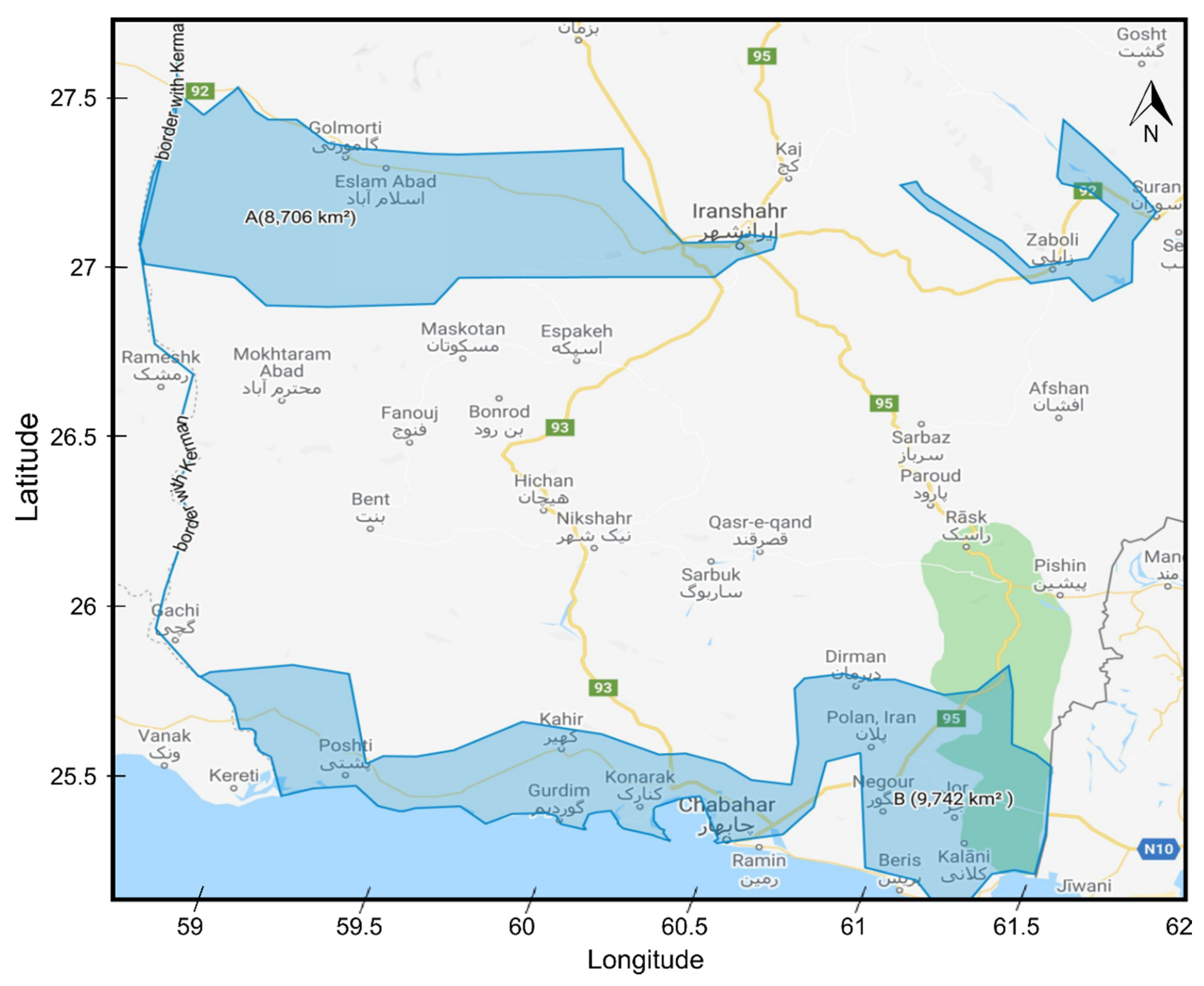
2. Study Area
3. Data Set Description
3.1. CYGNSS data
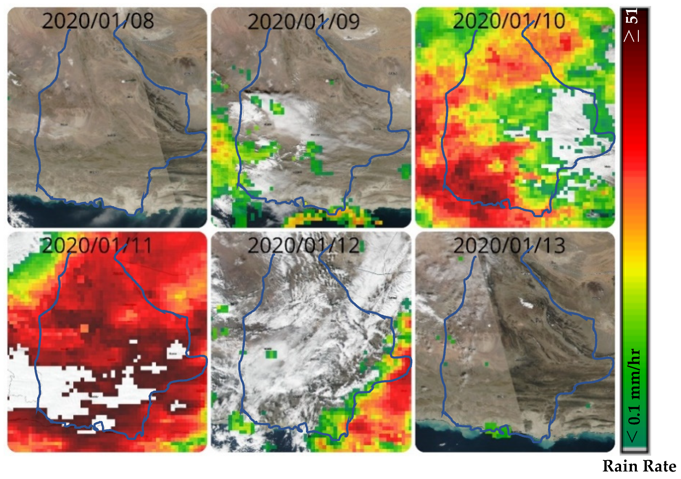
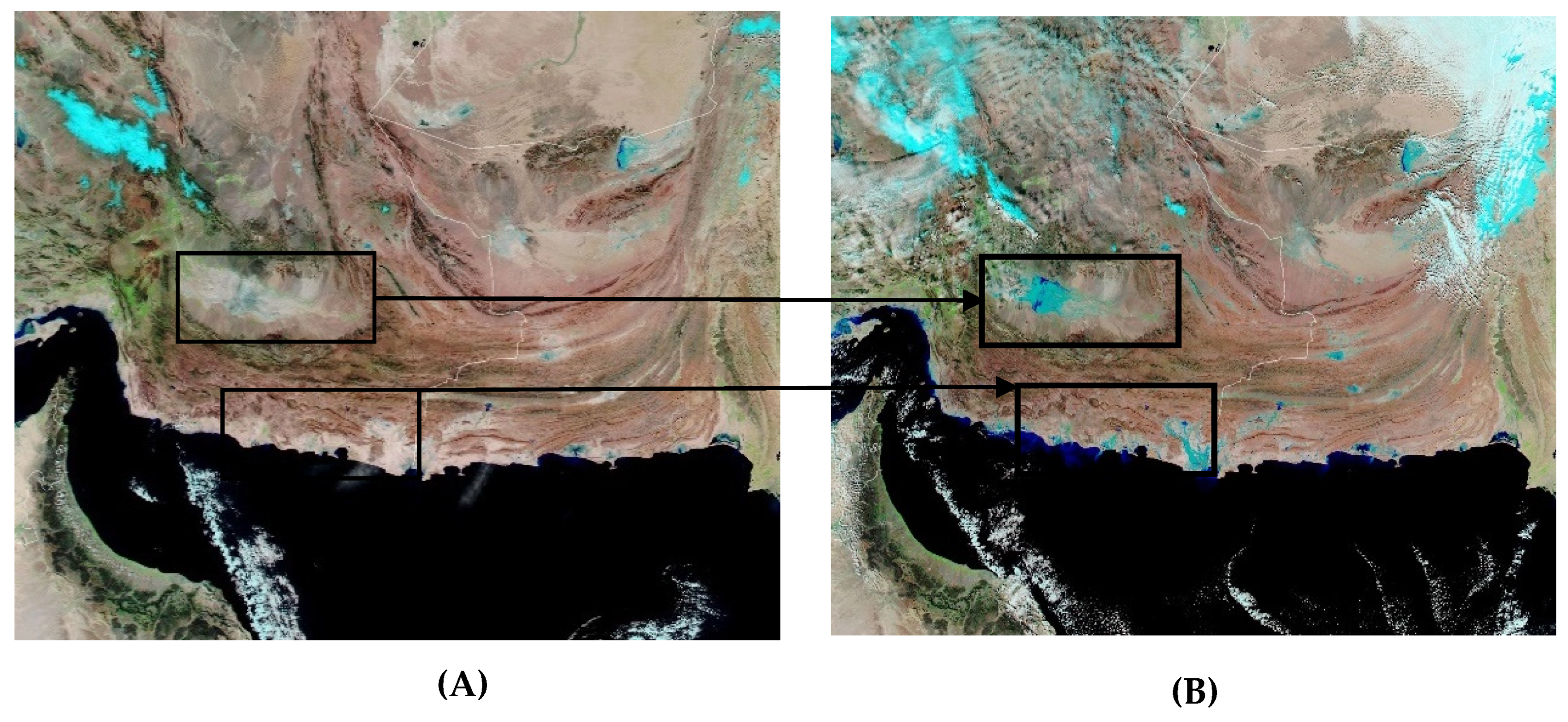
3.2. Satellite Image
4. Method and Discussion
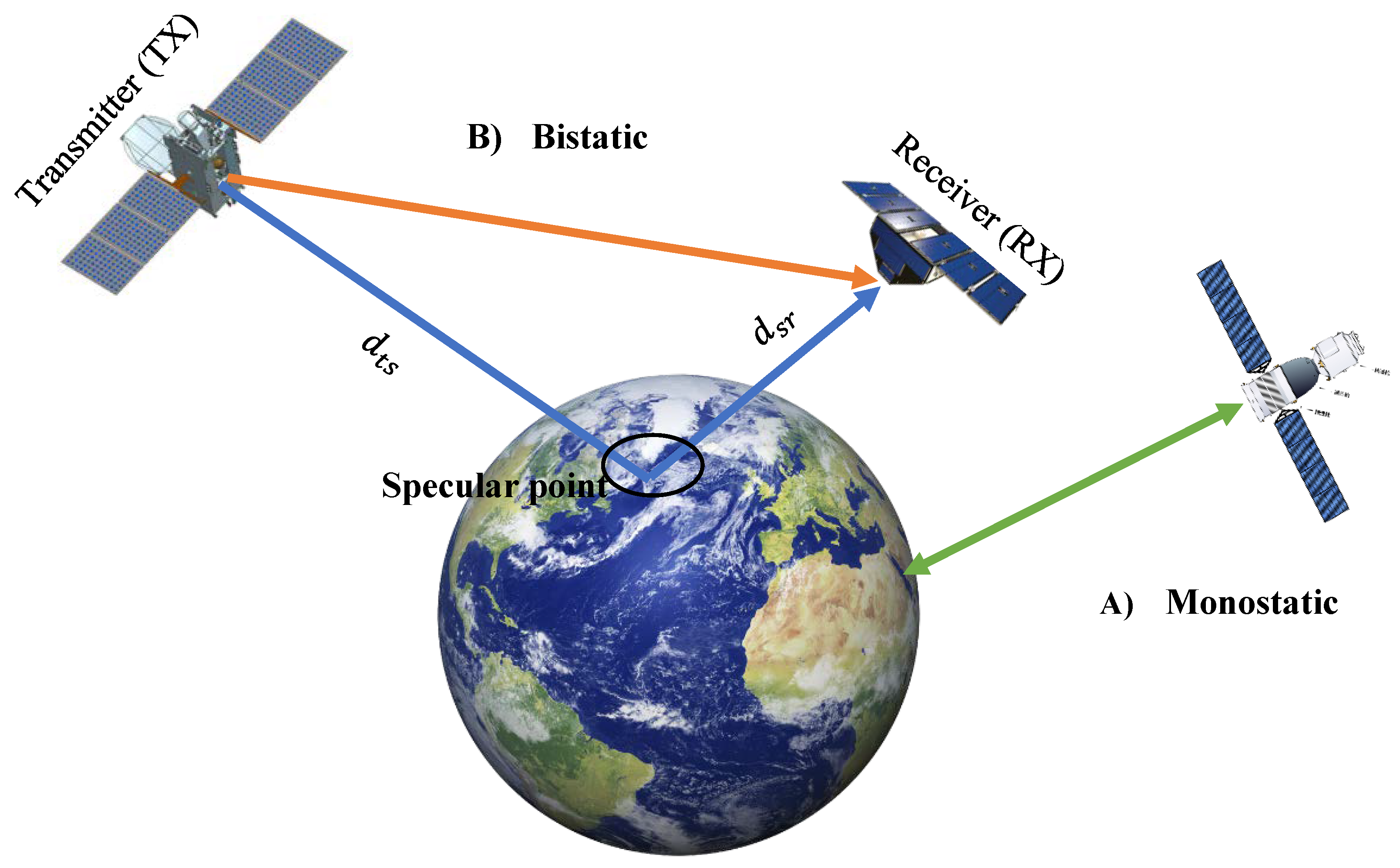
4.1. The Bistatic Radar Equations
- -
- ddm_snr ( with being the maximum value in a single DDM bin and is the average raw noise counts per-bin
- -
- gps_tx_power_db_w ()
- -
- gps_ant_gain_db_i ()
- -
- sp_rx_gain ()
- -
- rx_to_sp_range ()
- -
- tx_to_sp_range ()
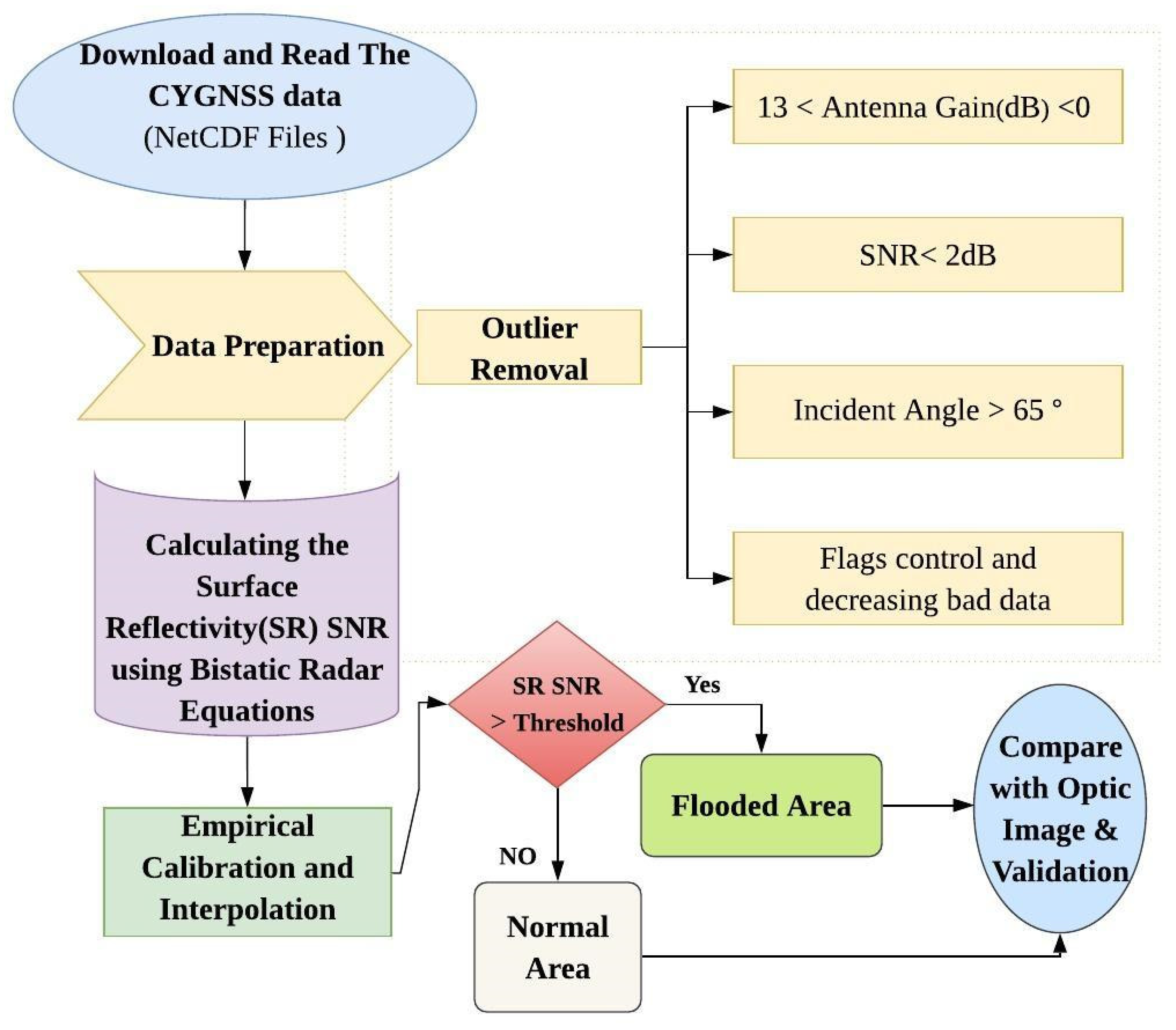
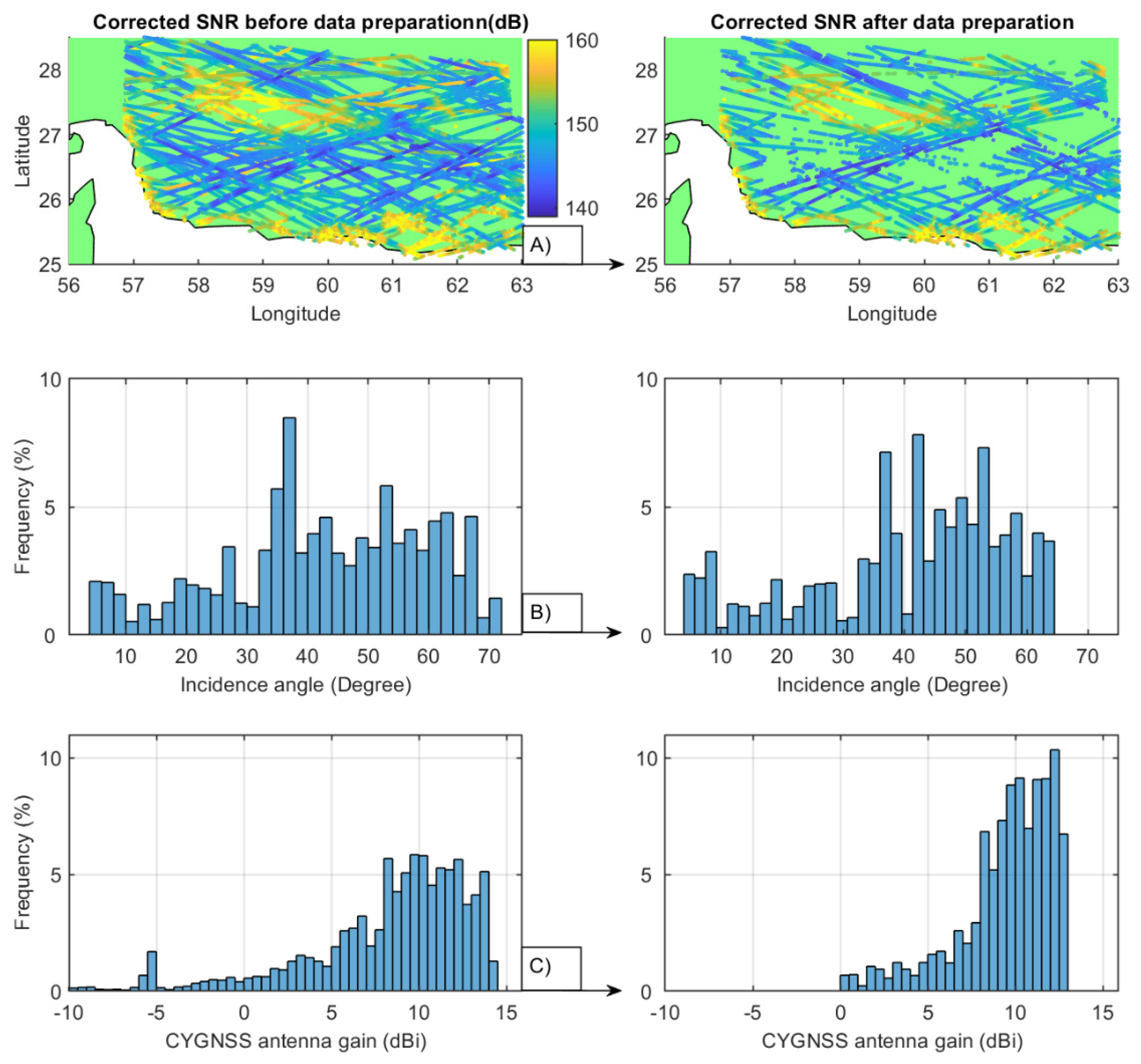
4.2. Data Preparation and Calibration
- GPS transmitter bias: GPS transmit powers are approximate estimates with some biases which should be considered. The main sources of these biases could be unknown transmitting powers of GPS satellites and the biases in associated with GPS pseudorandom noise (PRN) codes [16,44]. We used empirical calibration developed by Chew et al. (2018) for CYGNSS products. Table 3 shows the magnitude of the biases which should be corrected during the estimation of [15].
- Incidence angle: This parameter also affects a coherent reflection when the incidence angles are above 40 degrees or 50 degrees and was negligible for our purpose [34], but we deleted data with an incidence angle of more than 65 degrees.
- Quality Control Flags: The Level 1A data product used in this study was refined by applying a set of quality control flags designed and included in the data to indicate potential problems [27,45]. The specific flags we used were 2, 4, 5, 8, 16, and 17, which were related to S-band transmitter powered up, spacecraft attitude error, black body DDM, DDM is a test pattern, the direct signal in DDM, and low confidence in the GPS EIR estimate, respectively. Based on the work by Chew et al. (2018) on soil moisture, we removed data with those quality flags in this study.
- Additional correction and removal: We removed data with less than 2dB and CYGNSS antenna gain of less than 0 dB or more than 13 dB. These corrections were empirical and are not standardized, but have been shown to be beneficial [16].
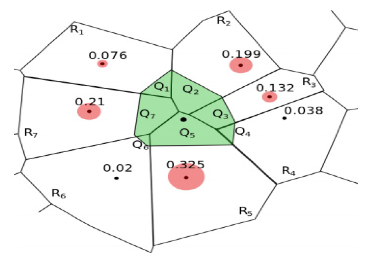
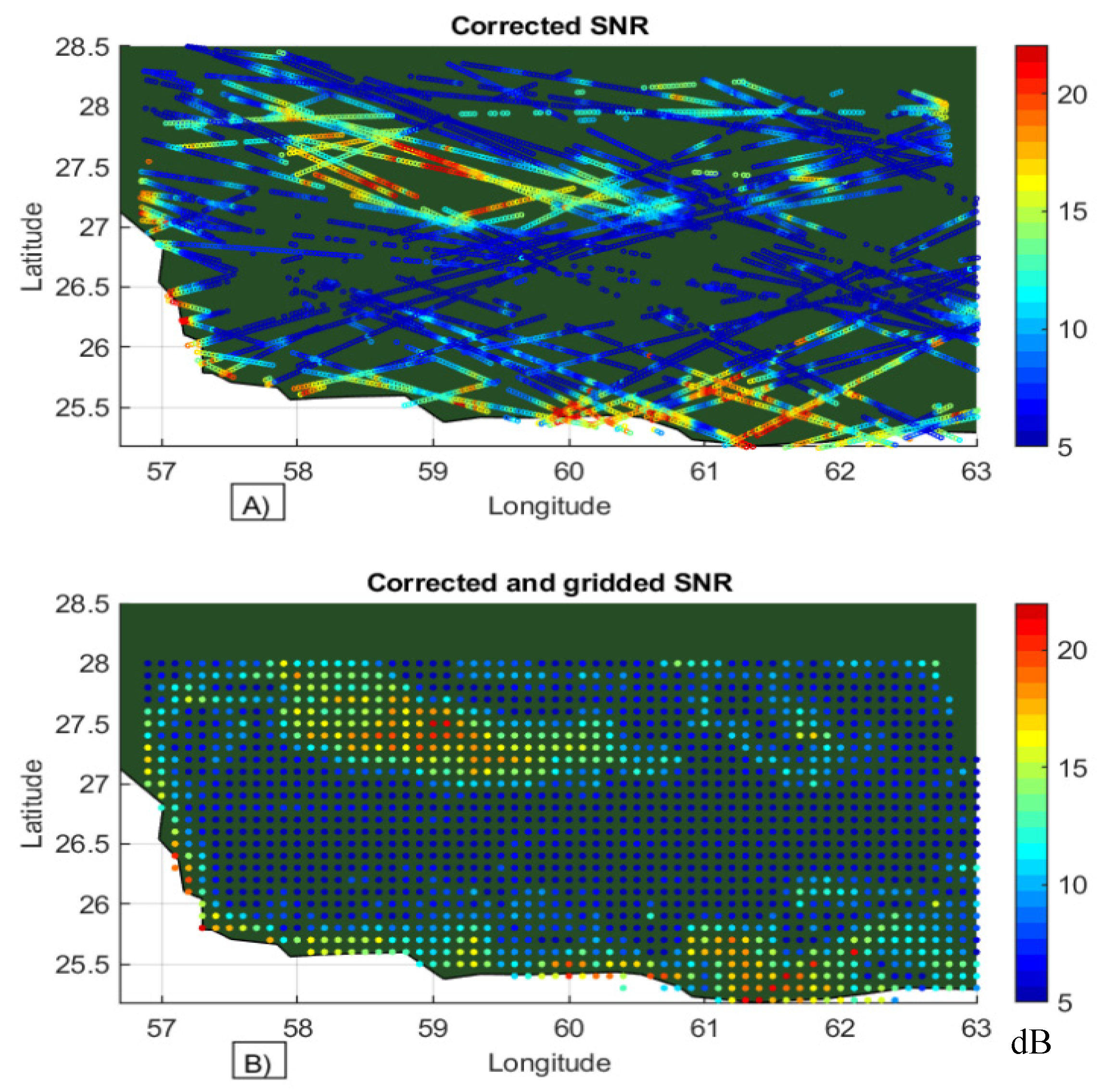
4.3. Interpolation
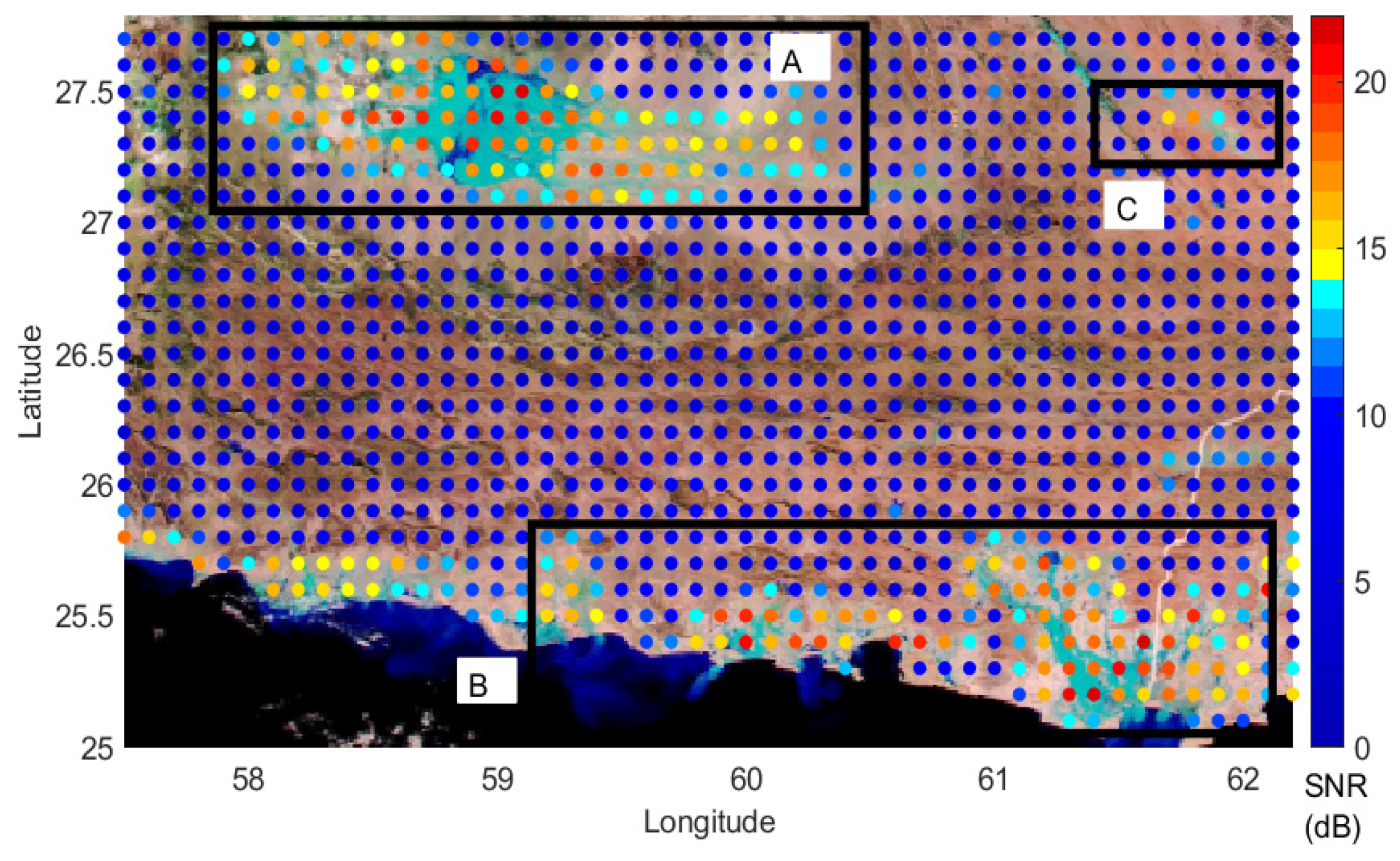
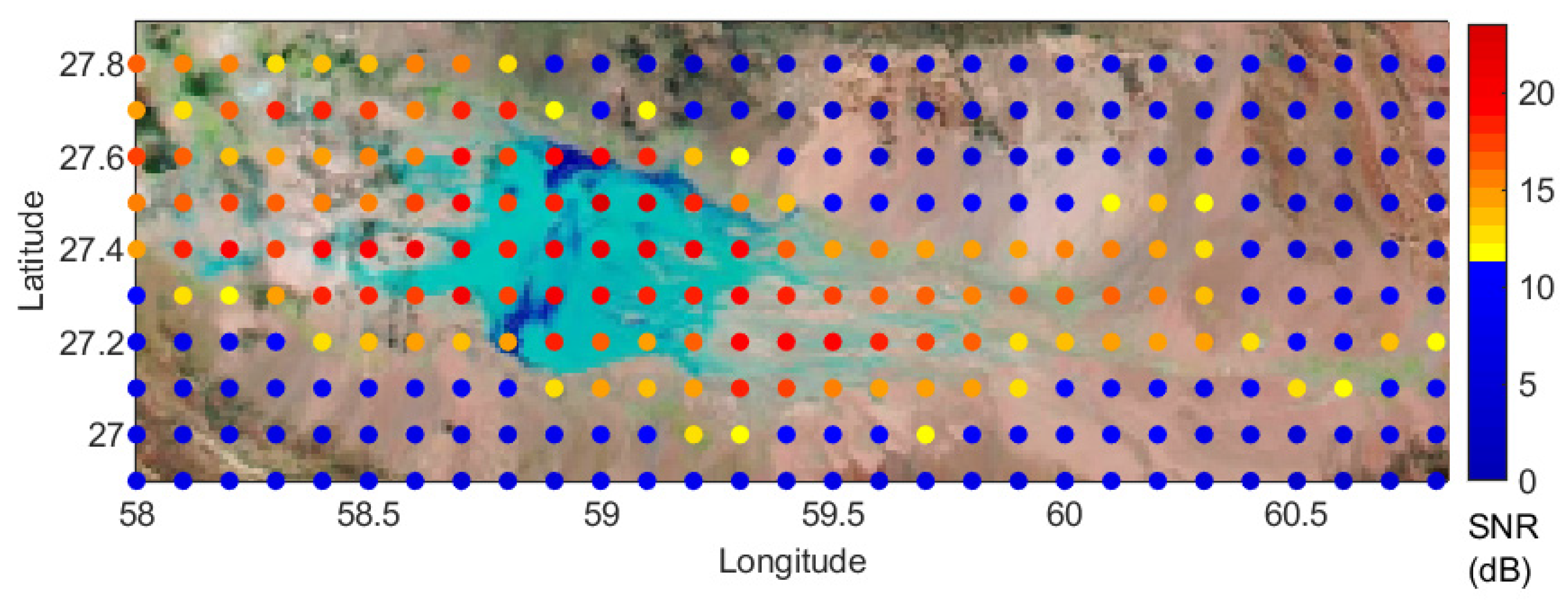
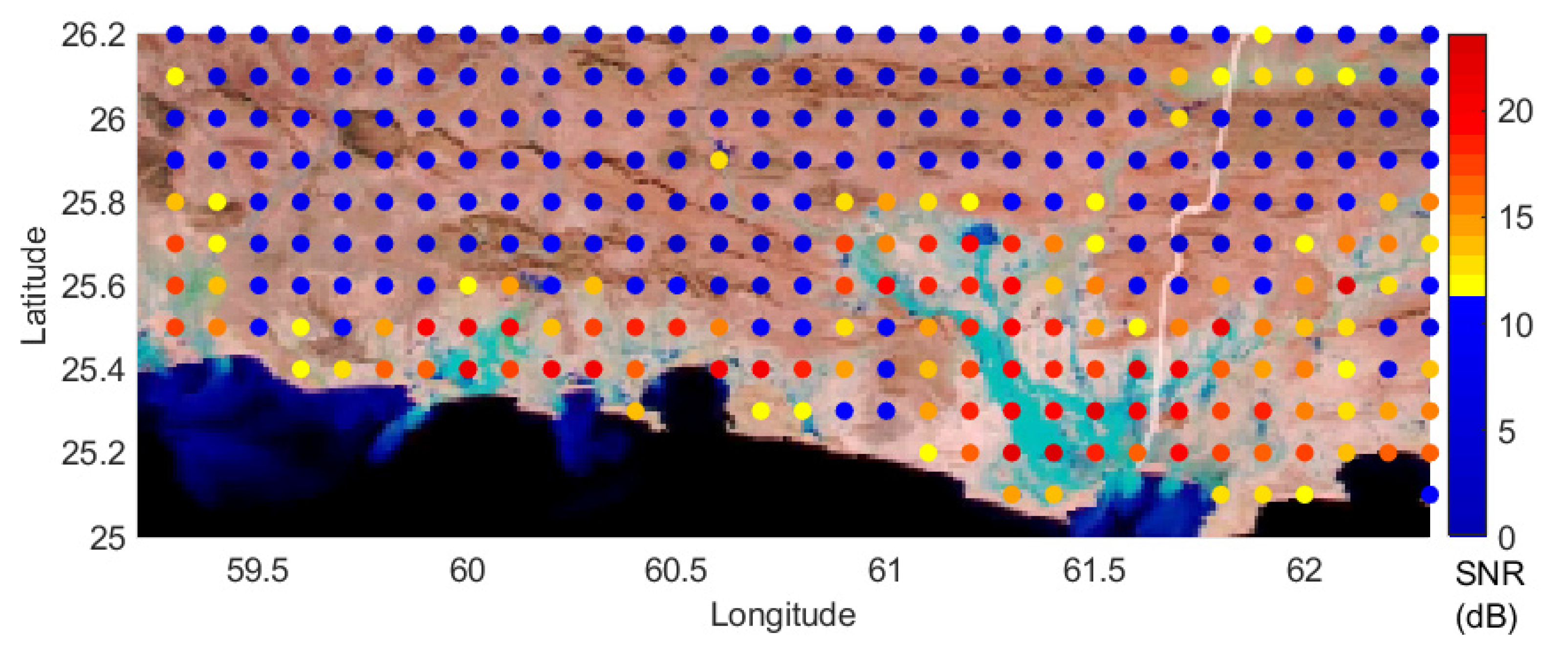
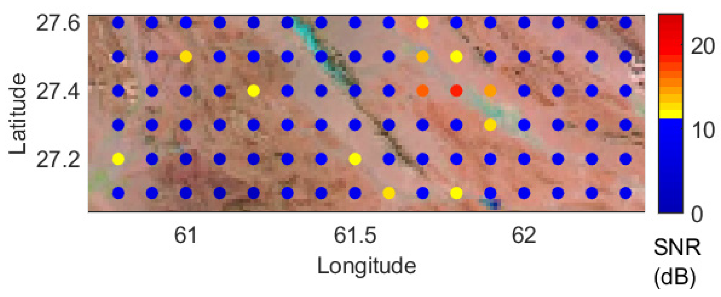
4.4. Evaluation and Mapping
5. Summary and Conclusions
Author Contributions
Funding
Acknowledgments
Conflicts of Interest
References
- Van Westen, C. Remote sensing for natural disaster management. Int. Arch. Photogramm. Remote Sens. 2000, 33, 1609–1617. [Google Scholar]
- Salami, R.O.; von Meding, J.K.; Giggins, H. Vulnerability of Human Settlements to Flood Risk in the Core Area of Ibadan Metropolis, Nigeria. Jàmbá J. Disaster Risk Stud. 2017, 9, 1–14. [Google Scholar] [CrossRef] [PubMed]
- ADPC; UNDP. Integrated Flood Risk Management in Asia; A Primer ADPC: Bangkok, Thailand, 2005. [Google Scholar]
- Abidin, H.Z.; Andreas, H.; Gumiar, I.; Sidiq, T.P.; Gamal, M. Environmental impacts of land subsidence in urban areas of Indonesia. In FIG Working Week; TS 3—Positioning and Measurement: Sofia, Bulgaria, 2015. [Google Scholar]
- Nash, L.L. The Colorado River Basin and Climatic Change: The Sensitivity of Streamflow and Water Supply to Variations in Temperature and Precipitation; US Environmental Protection Agency, Office of Policy, Planning, and Evaluation: Washington, DC, USA, 1993.
- Houston, J. Variability of precipitation in the Atacama Desert: Its causes and hydrological impact. Int. J. Clim. J. R. Meteorol. Soc. 2006, 26, 2181–2198. [Google Scholar] [CrossRef]
- Brivio, P.A.; Colombo, R.; Maggi, M.; Tomasoni, R. Integration of remote sensing data and GIS for accurate mapping of flooded areas. Int. J. Remote Sens. 2002, 23, 429–441. [Google Scholar] [CrossRef]
- CNN. Available online: https://edition.cnn.com/2019/04/07/middleeast/iran-flood-fatalities/index.html. (accessed on 7 April 2019).
- Oberstadler, R.; Hönsch, H.; Huth, D. Assessment of the mapping capabilities of ERS-1 SAR data for flood mapping: A case study in Germany. Hydrol. Process. 1997, 11, 1415–1425. [Google Scholar] [CrossRef]
- Kuenzer, C.; Guo, H.; Huth, J.; Leinenkugel, P.; Li, X.; Dech, S. Flood mapping and flood dynamics of the Mekong Delta: ENVISAT-ASAR-WSM based time series analyses. Remote Sens. 2013, 5, 687–715. [Google Scholar] [CrossRef]
- Chew, C.; Reager, J.T.; Small, E. CYGNSS data map flood inundation during the 2017 Atlantic hurricane season. Sci. Rep. 2018, 8, 1–8. [Google Scholar] [CrossRef]
- Rajabi, M.; Amiri-Simkooei, A.R.; Asgari, J.; Nafisi, V.; Kiaei, S. Analysis of TEC time series obtained from global ionospheric maps. J. Geomat. Sci. Technol. 2015, 4, 213–224. [Google Scholar]
- Rajabi, M.; Amiri-Simkooei, A.R.; Nahavandchi, H.; Nafisi, V. Modeling and Prediction of Regular Ionospheric Variations and Deterministic Anomalies. Remote Sens. 2020, 12, 936. [Google Scholar] [CrossRef]
- Tabibi, S. Snow Depth and Soil Moisture Retrieval Using SNR-Based GPS and GLONASS Multipath Reflectometry. Ph.D. Thesis, University of Luxembourg, Luxembourg, 2016. [Google Scholar]
- Li, W.; Cardellach, E.; Fabar, F.; Rius, A.; Ribó, S.; Martín-Neira, M. First spaceborne phase altimetry over sea ice using TechDemoSat-1 GNSS-R signals. Geophys. Res. Lett. 2017, 44, 8369–8376. [Google Scholar] [CrossRef]
- Chew, C.; Small, E. Soil moisture sensing using spaceborne GNSS reflections: Comparison of CYGNSS reflectivity to SMAP soil moisture. Geophys. Res. Lett. 2018, 45, 4049–4057. [Google Scholar] [CrossRef]
- Wu, X.; Li, Y.; Xu, J. Theoretical study on GNSS-R vegetation biomass. In Proceedings of the 2012 IEEE International Geoscience and Remote Sensing Symposium, Munich, Germany, 12 November 2012. [Google Scholar]
- Wan, W.; Liu, B.; Zeng, Z.; Chen, X. Using CYGNSS data to monitor China’s flood inundation during typhoon and extreme precipitation events in 2017. Remote Sens. 2019, 11, 854. [Google Scholar] [CrossRef]
- Hoseini, M.; Asgarimehr, M.; Zavorotny, V.; Nahavandchi, H.; Ruf, C.; Wickert, J. First evidence of mesoscale ocean eddies signature in GNSS reflectometry measurements. Remote Sens. 2020, 12, 542. [Google Scholar] [CrossRef]
- Clarizia, M.P.; Ruf, C.S. Wind speed retrieval algorithm for the Cyclone Global Navigation Satellite System (CYGNSS) mission. IEEE Trans. Geosci. Remote Sens. 2016, 54, 4419–4432. [Google Scholar] [CrossRef]
- Liu, B.; Wan, W.; Hong, Y. Can the Accuracy of Sea Surface Salinity Measurement Be Improved by Incorporating Spaceborne GNSS-Reflectometry? IEEE Geosci. Remote Sens. Lett. 2020. [Google Scholar] [CrossRef]
- Zavorotny, V.U.; Gleason, S.; Cardellach, E.; Camps, A. Tutorial on remote sensing using GNSS bistatic radar of opportunity. IEEE Geosci. Remote Sens. Mag. 2014, 2, 8–45. [Google Scholar] [CrossRef]
- Eroglu, O.; Kurum, M.; Boyd, D.; Gurbuz, A.C. High Spatio-Temporal Resolution CYGNSS Soil Moisture Estimates Using Artificial Neural Networks. Remote Sens. 2019, 11, 2272. [Google Scholar] [CrossRef]
- Teunissen, P.; Montenbruck, O. Springer Handbook of Global Navigation Satellite Systems; Springer: Cham, Switzerland, 2017. [Google Scholar]
- Guerriero, L.; Pierdicca, N.; Egido, A.; Caparrini, M.; Paloscia, S.; Santi, E.; Floury, N. Modeling of the GNSS-R signal as a function of soil moisture and vegetation biomass. In Proceedings of the 2013 IEEE International Geoscience and Remote Sensing Symposium-IGARSS, Melbourne, VIC, Australia, 21–26 July 2013. [Google Scholar]
- Masters, D.; Axelrad, P.; Katzberg, S. Initial results of land-reflected GPS bistatic radar measurements in SMEX02. Remote Sens. Environ. 2004, 92, 507–520. [Google Scholar] [CrossRef]
- Ruf, C.; Chang, P.S.; Clarizia, M.P.; Gleason, S.; Jelenak, Z. CYGNSS Handbook; Michigan Pub: Ann Arbor, MI, USA, 2016; p. 154. [Google Scholar]
- Ruf, C.S.; Atlas, R.; Chang, P.S.; Clarizia, M.P.; Garrison, J.; Gleason, S.; Katzberg, S.; Jelenak, Z.; Johnson, J.; Sharanya, J.; et al. New ocean winds satellite mission to probe hurricanes and tropical convection. Bull. Am. Meteorol. Soc. 2016, 97, 385–395. [Google Scholar] [CrossRef]
- Ruf, C.S.; Chew, C.; Lang, T.; Morris, M.; Nave, K.; Ridley, A.; Balasubramaniam, R. A new paradigm in earth environmental monitoring with the CYGNSS small satellite constellation. Sci. Rep. 2018, 8, 1–13. [Google Scholar] [CrossRef]
- Zribi, M.; Gorrab, A.; Baghdadi, N.; Lili-Chabaane, Z.; Mougenot, B. Influence of radar frequency on the relationship between bare surface soil moisture vertical profile and radar backscatter. IEEE Geosci. Remote Sens. Lett. 2013, 11, 848–852. [Google Scholar] [CrossRef]
- Camps, A.; Park, H.; Pablos, M.; Foti, G.; Gommenginger, C.; Liu, P.W.; Jugge, J. Sensitivity of GNSS-R spaceborne observations to soil moisture and vegetation. IEEE J. Sel. Top. Appl. Earth Obs. Remote Sens. 2016, 9, 4730–4742. [Google Scholar] [CrossRef]
- Chew, C.; Shah, R.; Zuffada, Z.; Hajj, G.; Masters, D.; Mannuci, A. Demonstrating soil moisture remote sensing with observations from the UK TechDemoSat-1 satellite mission. Geophys. Res. Lett. 2016, 43, 3317–3324. [Google Scholar] [CrossRef]
- Gerlein-Safdi, C.; Ruf, C.S. A CYGNSS-based algorithm for the detection of inland waterbodies. Geophys. Res. Lett. 2019, 46, 12065–12072. [Google Scholar] [CrossRef]
- Morris, M.; Chew, C.; Reager, J.; Shah, R.; Zuffada, C. A novel approach to monitoring wetland dynamics using CYGNSS: Everglades case study. Remote Sens. Environ. 2019, 233, 111417. [Google Scholar] [CrossRef]
- Amineh, Z.B.A.; Hashemian, S.J.A.-D.; Magholi, A. Integrating Spatial Multi Criteria Decision Making (SMCDM) with Geographic Information Systems (GIS) for delineation of the most suitable areas for aquifer storage and recovery (ASR). J. Hydrol. 2017, 551, 577–595. [Google Scholar] [CrossRef]
- World Data. Available online: https://www.worlddata.info (accessed on 1 February 2020).
- Huffman, G.J.; Bolvin, D.T.; Nelkin, E.J. Integrated Multi-satellitE Retrievals for GPM (IMERG) technical documentation. NASA/GSFC Code 2015, 612, 47. [Google Scholar]
- Lindsey, R.; Herring, D.; Abbott, M.; Conboy, B.; Esaias, W. MODIS Brochure; Goddard Space Flight Center: Greenbelt, MD, USA, 2013. [Google Scholar]
- Flash Flooding in Iran. 2020. Available online: https://earthobservatory.nasa.gov/images/146150/flash-flooding-in-iran (accessed on 1 February 2020).
- Eaves, J.L. Introduction to radar. In Principles of Modern Radar; Van Nostrand Reinhold; Springer: New York, NY, USA, 1987; pp. 1–27. [Google Scholar]
- Bruder, J.A. IEEE Radar standards and the radar systems panel. IEEE Aerosp. Electron. Syst. Mag. 2013, 28, 19–22. [Google Scholar] [CrossRef]
- Nghiem, S.V.; Zuffada, C.; Shah, R.; Chew, C.; Lowe, S.T.; Mannucci, A.J.; Cardellach, E.; Brakenridge, G.R.; Geller, G.; Rosenqvist, A. Wetland monitoring with global navigation satellite system reflectometry. Earth Space Sci. 2017, 4, 16–39. [Google Scholar] [CrossRef]
- Masters, D. Surface Remote Sensing Applications of GNSS Bistatic Radar: Soil Moisture and Aircraft Altimetry. Ph.D. Thesis, University of Colorado, Boulder, CO, USA, 2004. [Google Scholar]
- Wang, T.; Ruf, C.S.; Block, B.; McKague, D.; Gleason., S. Characterization of GPS L1 EIRP: Transmit power and antenna gain pattern. In Proceedings of the 31st ION GNSS, Miami, FL, USA, 24–28 September 2018. [Google Scholar]
- Basis, A.T. Cyclone Global Navigation Satellite System (CYGNSS). Prepared by: Maria Paola Clarizia, University of Michigan, Valery Zavorotny, NOAA. 2015. [Google Scholar]
- Sibson, R. A Brief Description of Natural Neighbor Interpolation (Chapter 2); Barnett, V., Ed.; Interpolating Multivariate Data; John Wiley: Chichester, UK, 1981; pp. 21–36. [Google Scholar]
- Voronoi, G. Nouvelles applications des paramètres continus à la théorie des formes quadratiques. Deuxième mémoire. Recherches sur les parallélloèdres primitifs. J. für die reine und angewandte Mathematik (Crelles J.) 1908, 1908, 198–287. [Google Scholar] [CrossRef]
- Tsidaev, A. Parallel algorithm for natural neighbor interpolation. In Proceedings of the 2nd Ural Workshop on Parallel, Distributed, and Cloud Computing for Young Scientists, Yekaterinburg, Russia, 6 October 2016. [Google Scholar]
- Harrison, J. The Jaz Murian depression, Persian Baluchistan. Geogr. J. 1943, 101, 206–225. [Google Scholar] [CrossRef]
- Frs, N.F. From Musandam to the Iranian Makran. Geogr. J. 1975, 141, 55–58. [Google Scholar] [CrossRef]


| Parameters | Description |
|---|---|
| Orbit | LEO, ~520 km, Nonsynchronous |
| Period | 95.1 min |
| Spatial Resolution | ∼25 km × 25 km (incoherent), ∼0.5 km × 5 km (coherent, theoretical) |
| Revisit Times | 2.8 h median, 7.2 h mean |
| Polarization of the reflectometry antennas | LHCP |
| Coverage | −38 < Latitude < 38 & −180 < Longitude < 180 |
| Type of Data which is relevant | Observe GPS L1 C/A signals and Delay Doppler Maps |
| Parameters | Description |
|---|---|
| ddm_snr | Delay Doppler Map (DDM) signal-to-noise ratio, in dB |
| gps_tx_power_db_w | GPS transmit power, in dB. |
| rx_to_sp_range | Distance between the CYGNSS spacecraft and the specular point, in meters. |
| tx_to_sp_range | Distance between the GPS spacecraft and the specular point, in meters. |
| gps_ant_gain_db_i | GPS transmit antenna gain. Antenna gain in the direction of the specular point, in dBi |
| sp_rx_gain | Specular point Rx antenna gain. The receive antenna gains in the direction of the specular point, in decibel isotropic (dBi). |
| quality_flags | Per-DDM quality flags |
| sp_lat | Specular point latitude, in degrees North |
| sp_lon | Specular point longitude, in degrees East |
| sp_inc_angle | The specular point incidence angle, in degrees |
| PRN | Bias (dB) | PRN | Bias (dB) | PRN | Bias (dB) | PRN | Bias (dB) |
|---|---|---|---|---|---|---|---|
| 1 | 1.017 | 9 | 1.498 | 17 | 0.256 | 25 | 0.880 |
| 2 | 0.004 | 10 | −0.783 | 18 | −0.206 | 26 | 0.163 |
| 3 | 1.636 | 11 | −0.230 | 19 | −0.206 | 27 | 0.409 |
| 4 | - | 12 | −1.021 | 20 | 0.345 | 28 | −0.712 |
| 5 | −0.610 | 13 | 0.007 | 21 | −0.909 | 29 | −1.032 |
| 6 | 0.24 | 14 | −0.730 | 22 | −0.838 | 30 | 0.877 |
| 7 | −0.709 | 15 | −0.376 | 23 | −0.858 | 31 | −0.562 |
| 8 | 0.605 | 16 | −0.481 | 24 | 1.140 | 32 | −0.819 |
© 2020 by the authors. Licensee MDPI, Basel, Switzerland. This article is an open access article distributed under the terms and conditions of the Creative Commons Attribution (CC BY) license (http://creativecommons.org/licenses/by/4.0/).
Share and Cite
Rajabi, M.; Nahavandchi, H.; Hoseini, M. Evaluation of CYGNSS Observations for Flood Detection and Mapping during Sistan and Baluchestan Torrential Rain in 2020. Water 2020, 12, 2047. https://doi.org/10.3390/w12072047
Rajabi M, Nahavandchi H, Hoseini M. Evaluation of CYGNSS Observations for Flood Detection and Mapping during Sistan and Baluchestan Torrential Rain in 2020. Water. 2020; 12(7):2047. https://doi.org/10.3390/w12072047
Chicago/Turabian StyleRajabi, Mahmoud, Hossein Nahavandchi, and Mostafa Hoseini. 2020. "Evaluation of CYGNSS Observations for Flood Detection and Mapping during Sistan and Baluchestan Torrential Rain in 2020" Water 12, no. 7: 2047. https://doi.org/10.3390/w12072047
APA StyleRajabi, M., Nahavandchi, H., & Hoseini, M. (2020). Evaluation of CYGNSS Observations for Flood Detection and Mapping during Sistan and Baluchestan Torrential Rain in 2020. Water, 12(7), 2047. https://doi.org/10.3390/w12072047