Hydropower Potential in the Alps under Climate Change Scenarios. The Chavonne Plant, Val D’Aosta


Abstract
1. Introduction
2. Literature Review
- (i)
- We used Poli-Hydro, a semi-distributed model, fully accounting for changes in cryospheric process under climate change, including glaciers’ flow/melting, and snow cover accumulation/depletion, so gathering scenarios that were largely significant from the hydrological point of view;
- (ii)
- We originally provided climate, and hydrological scenarios in this part of Italy, using the latest, most recently released climate scenarios of the AR6 of the IPCC, unexploited hitherto as far as we know;
- (iii)
- We studied for the first time to our knowledge, present and future hydro-power productivity in the Val d’Aosta valley, and particularly in the Gran Paradiso National Park area, an area of tremendous ecological value, and displaying a very large hydropower potential, to be properly exploited henceforward.
3. Data and Methods
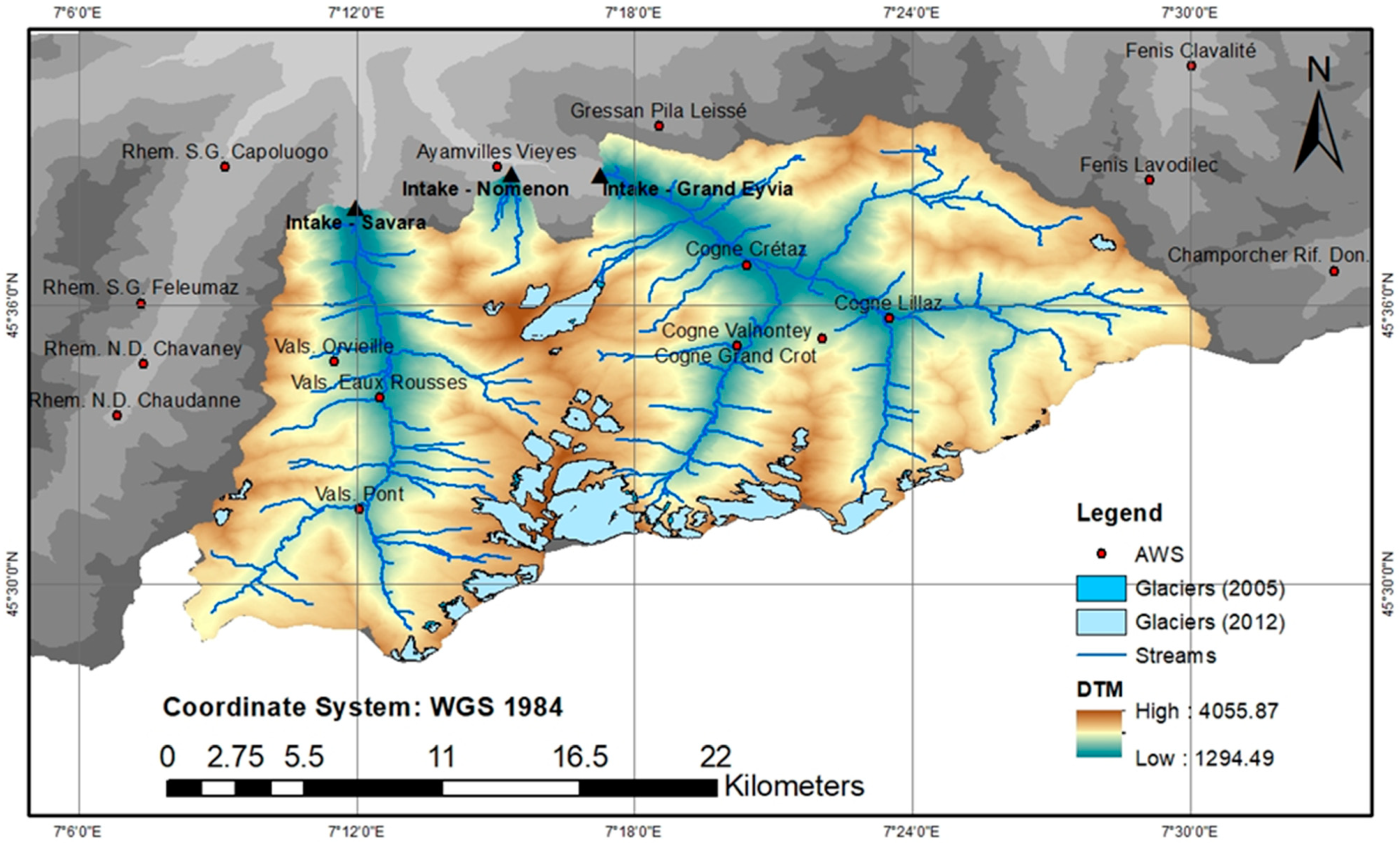
3.1. Case Study
3.2. Hydro-Meteorological Data (2005–2018)
3.3. Glacier’s Cover Dynamics, Climate and Hydropower Projections (2019–2100)
3.4. Ice Flow Modelling and Mass Balance
3.5. Hydrological Model
3.6. Hydrological and Hydropower Projections
4. Results
4.1. Model Tuning, and Hydrological Projections
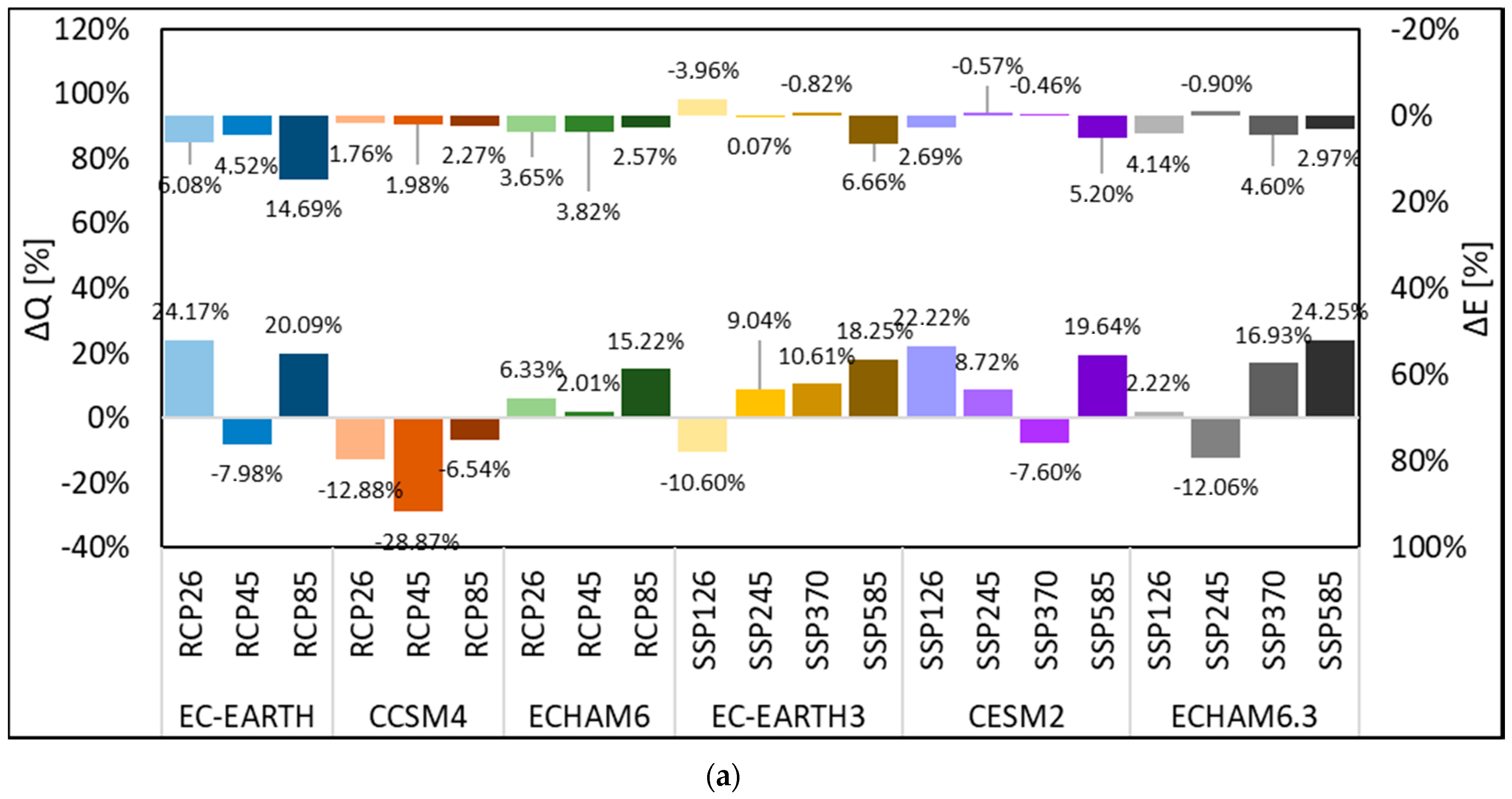
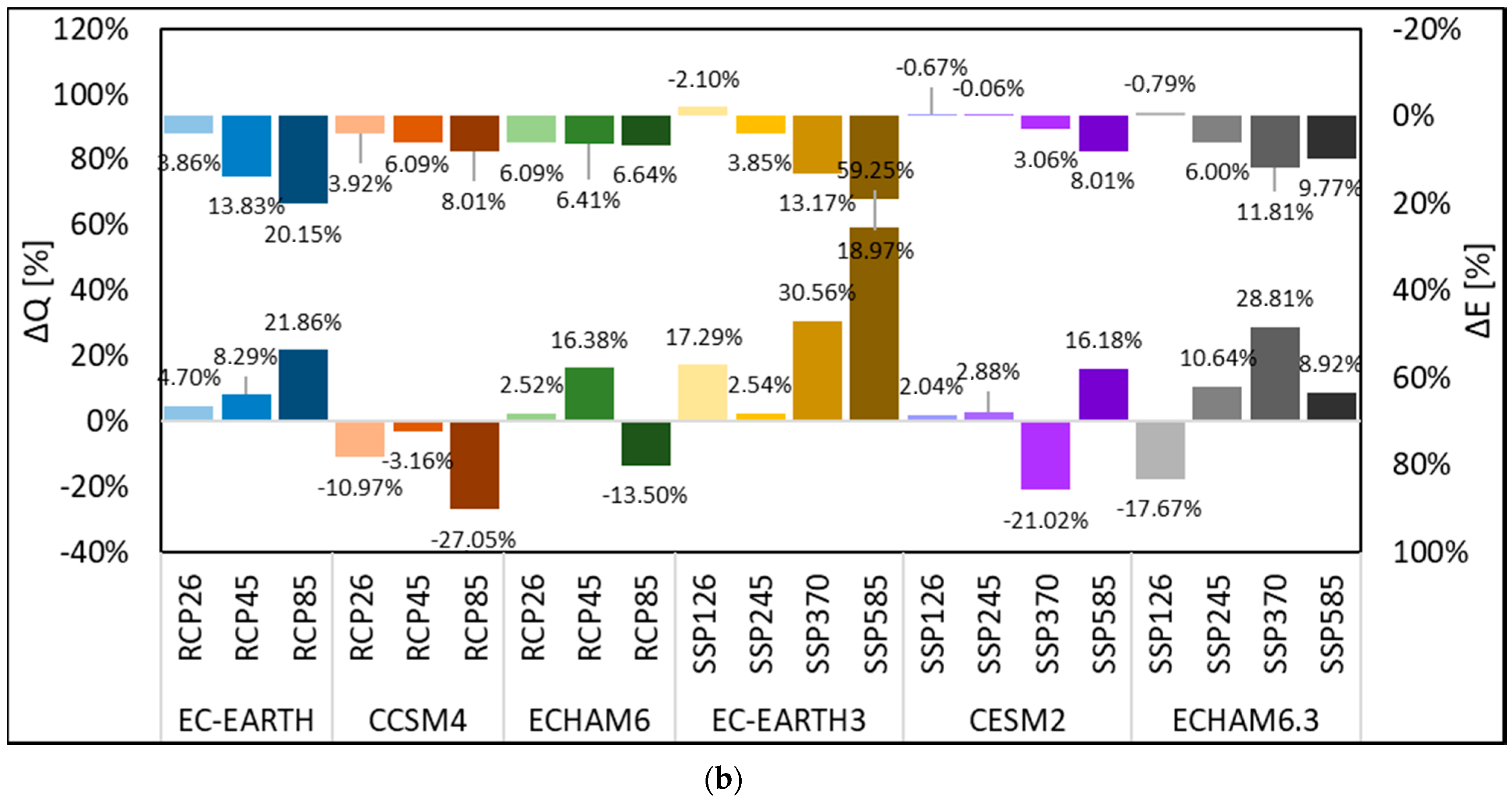
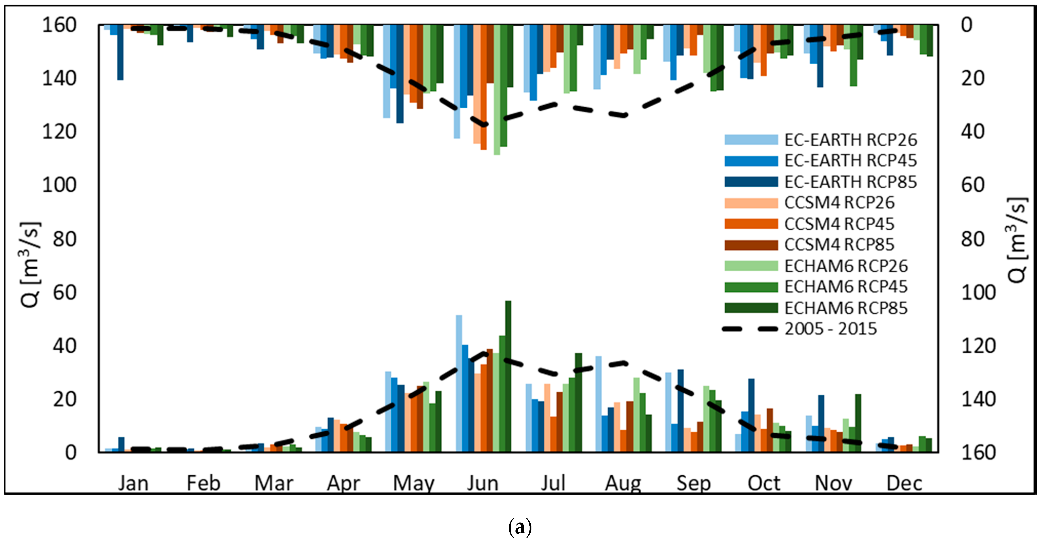
4.2. Mean Hydrological and Hydropower Scenarios
5. Discussion
5.1. Cryospheric Water under Future Climate Change
5.2. Hydropower Production under Climate Change
5.3. Limitations and Outlooks
6. Conclusions
Author Contributions
Funding
Acknowledgments
Conflicts of Interest
References
- Barnett, T.P.; Adam, J.C.; Lettenmaier, D.P. Potential impacts of a warming climate on water availability in snow-dominated regions. Nature 2005, 438, 9. [Google Scholar] [CrossRef]
- Viganò, G.; Confortola, G.; Fornaroli, R.; Cabrini, R.; Canobbio, S.; Mezzanotte, V. Effects of future climate change on a river habitat in an italian alpine catchment. J. Hydrol. Eng. 2016, 21, 1–14. [Google Scholar] [CrossRef]
- Soncini, A.; Bocchiola, D.; Azzoni, R.S.; Diolaiuti, G. A methodology for monitoring and modeling of high altitude Alpine catchments. Prog. Phys. Geogr. 2017, 41, 393–420. [Google Scholar] [CrossRef]
- Aili, T.; Soncini, A.; Bianchi, A.; Diolaiuti, G.; D’Agata, C.; Bocchiola, D. Assessing water resources under climate change in high-altitude catchments: A methodology and an application in the Italian Alps. Theor. Appl. Climatol. 2019, 135, 56–135. [Google Scholar] [CrossRef]
- D’Agata, C.; Bocchiola, D.; Soncini, A.; Maragno, D.; Smiraglia, C.; Diolaiuti, G.A. Recent area and volume loss of Alpine glaciers in the Adda River of Italy and their contribution to hydropower production. Cold Reg. Sci. Technol. 2018, 148, 84–172. [Google Scholar] [CrossRef]
- D’Agata, C.; Bocchiola, D.; Maragno, D.; Smiraglia, C.; Diolaiuti, G. Glacier Shrinkage Driven by Climate Change during Half a Century (1954–2007) in the Ortles-Cevedale Group. Theor. Appl. Climatol. 2014, 116, 169–190. [Google Scholar] [CrossRef]
- Diolaiuti, G.; Bocchiola, D.; D’agata, C.; Smiraglia, C. Evidence of climate change impact upon glaciers’ recession within the Italian Alps: The case of Lombardy glaciers. Theor. Appl. Climatol. 2012, 109, 45–429. [Google Scholar] [CrossRef]
- Diolaiuti, G.A.; Bocchiola, D.; Vagliasindi, M.; D’Agata, C.; Smiraglia, C. The 1975-2005 glacier changes in Aosta Valley (Italy) and the relations with climate evolution. Prog. Phys. Geogr. 2012, 36, 85–764. [Google Scholar] [CrossRef]
- Ravazzani, G.; Valle, F.D.; Gaudard, L.; Mendlik, T.; Gobiet, A.; Mancini, M. Assessing climate impacts on hydropower production: The case of the Toce river basin. Climiate 2016, 4, 16. [Google Scholar] [CrossRef]
- Bombelli, G.M.; Soncini, A.; Bianchi, A.; Bocchiola, D. Potentially modified hydropower production under climate change in the Italian Alps. Hydrol. Process 2019, 33, 1–18. [Google Scholar] [CrossRef]
- Patro, E.R.; De Michele, C.; Avanzi, F. Future perspectives of run-of-the-river hydropower and the impact of glaciers’ shrinkage: The case of Italian Alps. Appl. Energy 2018, 231, 699–713. [Google Scholar] [CrossRef]
- Bocchiola, D.; Rosso, R. The distribution of daily Snow water Equivalent in the Central Italian Alps. Adv. Water Resour. 2007, 30, 47–135. [Google Scholar]
- Valt, M.; Chiambretti, I.; Dellavedova, P. Fresh snow density on the Italian Alps. Geophys. Res. 2014, 16, 9715. [Google Scholar]
- Moss, R.H.; Edmonds, J.A.; Hibbard, K.A.; Manning, M.R.; Rose, S.K.; Van Vuuren, D.P. The next generation of scenarios for climate change research and assessment. Nature 2010, 463, 56–747. [Google Scholar] [CrossRef]
- Riahi, K.; Van Vuuren, D.P.; Kriegler, E.; Edmonds, J.; Neill, B.C.O.; Fujimori, S. The Shared Socioeconomic Pathways and their energy, land use, and greenhouse gas emissions implications: An overview. Glob. Environ. Chang. 2017, 42, 68–153. [Google Scholar] [CrossRef]
- Groppelli, B.; Soncini, A.; Bocchiola, D.; Rosso, R. Evaluation of future hydrological cycle under climate change scenarios in a mesoscale Alpine watershed of Italy. Nat. Hazards Earth Syst. Sci. 2011, 11, 85–1769. [Google Scholar] [CrossRef]
- Groppelli, B.; Bocchiola, D.; Rosso, R. Spatial downscaling of precipitation from GCMs for climate change projections using random cascades: A case study in Italy. Water Resour. Res. 2011, 47. [Google Scholar] [CrossRef]
- Soncini, A.; Bocchiola, D.; Confortola, G.; Bianchi, A.; Rosso, R.; Mayer, C. Future hydrological regimes in the upper Indus basin: A case study from a high-altitude glacierized catchment. J. Hydrometeorol. 2015, 16, 26–306. [Google Scholar] [CrossRef]
- Cuffey, K.M.; Oerlemans, J. Glaciers and climate change: A meteorologist’s view. J. Glaciol. 2002, 48, 173. [Google Scholar] [CrossRef][Green Version]
- Haeberli, W. Application of inventory data for estimating characteristics of and regional climate-change effects on mountain glaciers: A pilot study with the European Alps. Ann. Glaciol. 1995, 21, 206–212. [Google Scholar] [CrossRef]
- Carturan, L.; Baroni, C.; Brunetti, M.; Carton, A.; Fontana, G.D.; Salvatore, M.C. Analysis of the mass balance time series of glaciers in the Italian Alps. Cryosphere 2016, 10, 695–712. [Google Scholar] [CrossRef]
- Martinec, J.; Rango, A. Parameter values for snowmelt runoff modelling. J. Hydrol. 1986, 84, 197–219. [Google Scholar] [CrossRef]
- Akbari-Alashti, H.; Soncini, A.; Dinpashoh, Y.; Fakheri-Fard, A.; Talatahari, S.; Bocchiola, D. Operation of two major reservoirs of Iran under IPCC scenarios during the XXI century. Hydrol. Process 2018, 32, 71–3254. [Google Scholar] [CrossRef]
- Bocchiola, D.; Soncini, A. Water Resources Modeling and Prospective Evaluation in the Indus River Under Present and Prospective Climate Change. In Indus River Basin: Water Security and Sustainability; Khan, S., Adams, T., Eds.; Elsevier: Amsterdam, The Netherlands, 2019; pp. 17–56. [Google Scholar]
- Soncini, A.; Bocchiola, D.; Confortola, G.; Minora, U.; Vuillermoz, E.; Salerno, F. Future hydrological regimes and glacier cover in the Everest region: The case study of the upper Dudh Koshi basin. Sci. Total Environ. 2016, 565, 101–1084. [Google Scholar] [CrossRef] [PubMed]
- Hargreaves, G.H. Estimation of Potential and Crop Evapotranspiration. Trans. Am. Soc. Agric. Eng. 1974, 17, 4–701. [Google Scholar] [CrossRef]
- Ceriani, E.; Fiou, M. Impianto Idroelettrico di Chavonne—Studio di Impatto Ambientale. Regione Autonoma Valle D’Aosta, Ed.; 2010, p. 327. (In Italian). Available online: https://www.regione.vda.it/territorio/allegati/progetti_via_898_SINTESI.pdf (accessed on 14 July 2020).
- Confortola, G.; Soncini, A.; Bocchiola, D. Climate change will affect hydrological regimes in the Alps. Rev. géographie Alp 2014, 101-3. [Google Scholar] [CrossRef][Green Version]
- Grossi, G.; Caronna, P.; Ranzi, R. Hydrologic vulnerability to climate change of the Mandrone glacier (Adamello-Presanella group, Italian Alps). Adv. Water Resour. 2013, 55, 190–203. [Google Scholar] [CrossRef]
- Garavaglia, R.; Marzorati, A.; Confortola, G.; Bocchiola, D.; Lombardo, S.; Senese, A. Evoluzione del ghiacciaio dei Forni. Neve. E Valanghe 2018, 8, 60–67. [Google Scholar]
- Stucchi, L.; Bombelli, G.M.; Bianchi, A.; Bocchiola, D. Hydropower from the alpine cryosphere in the era of climate change. The case of the Sabbione storage plant in Italy. Water 2019, 11, 1599. [Google Scholar] [CrossRef]
- Faggian, P.; Giorgi, F. An analysis of global model projections over Italy, with particular attention to the Italian Greater Alpine Region (GAR). Clim. Chang. 2009, 96, 58–239. [Google Scholar] [CrossRef]
- Bocchiola, D.; Soncini, A.; Senese, A.; Diolaiuti, G. Modelling Hydrological Components of the Rio Maipo of Chile, and Their Prospective Evolution under Climate Change. Climiate 2018, 6, 57. [Google Scholar] [CrossRef]
- Fuss, S.; Canadell, J.G.; Peters, G.P.; Tavoni, M.; Andrew, R.M.; Ciais, P. COMMENTARY: Betting on negative emissions. Nat. Clim. Chang. 2014, 4, 3–850. [Google Scholar] [CrossRef]


| AWS | Latitude [°] | Longitude [°] | Altitude [m ASL] | T | Pl | H | S | R | W |
|---|---|---|---|---|---|---|---|---|---|
| Valsaverenche-Pont | 45.53 | 7.20 | 1951 | ✔ | ✔ | ✔ | ✔ | ✔ | |
| Valsaverenche-Eaux-Rousses | 45.57 | 7.21 | 1651 | ✔ | ✔ | ✔ | ✔ | ||
| Valsaverenche-Orvieille | 45.58 | 7.19 | 2170 | ✔ | ✔ | ✔ | |||
| Cogne-Lillaz | 45.60 | 7.39 | 1613 | ✔ | ✔ | ✔ | ✔ | ||
| Cogne-Grand-Crot | 45.59 | 7.37 | 2279 | ✔ | ✔ | ✔ | |||
| Cogne-Valnontey | 45.59 | 7.34 | 1682 | ✔ | ✔ | ✔ | |||
| Cogne-Crétaz | 45.61 | 7.34 | 1470 | ✔ | ✔ | ||||
| Gressan-Pila-Leissé | 45.66 | 7.31 | 2280 | ✔ | ✔ | ✔ | ✔ | ||
| Fenis-Clavalité | 45.69 | 7.50 | 1531 | ✔ | ✔ | ||||
| Fenis-Lavodilec | 45.64 | 7.49 | 2250 | ✔ | ✔ | ✔ | |||
| Champorcher-Rifugio-Dondena | 45.61 | 7.55 | 2181 | ✔ | ✔ | ✔ | |||
| Ayamvilles-Vieyes | 45.65 | 7.25 | 1139 | ✔ | ✔ | ||||
| Rhemes-Notre-Dame-Chaudanne | 45.56 | 7.11 | 1794 | ✔ | ✔ | ✔ | ✔ | ✔ | |
| Rhemes-Notre-Dame-Chavaney | 45.58 | 7.12 | 1690 | ✔ | ✔ | ✔ | ✔ | ||
| Rhemes-Saint-Georges-Feleumaz | 45.60 | 7.12 | 2325 | ✔ | ✔ | ✔ | |||
| Rhemes-Saint-Georges-Capoluogo | 45.65 | 7.15 | 1179 | ✔ | ✔ | ✔ |
| Parameter | Unit | Description | Value |
|---|---|---|---|
| TMFs,i | [mm day−1 °C−1] | Thermal melting factor, snow, ice | 1.59, 8 |
| RMFs,i | [mm day−1 W−1 m2] | Radiation melting factor, snow, ice | 4.4 × 10⁻³, 4.0 × 10⁻³ |
| K | [mm day−1] | Saturated conductivity | 5.45 |
| b | [.] | Ground flow exponent | 3.4 |
| θw, θw | [.] | Water content, wilting, field capacity | 0.15, 0.35 |
| fs | [m−1 year−1] | Ice flow basal sliding coefficient | 1.5 × 10⁻²¹ |
| fd | [m−1 year−1] | Ice flow deformation coefficient | 1.2 × 10⁻²⁴ |
| αs,i | [.] | Albedo, snow, ice | 0.3, 0.7 |
© 2020 by the authors. Licensee MDPI, Basel, Switzerland. This article is an open access article distributed under the terms and conditions of the Creative Commons Attribution (CC BY) license (http://creativecommons.org/licenses/by/4.0/).
Share and Cite
Duratorre, T.; Bombelli, G.M.; Menduni, G.; Bocchiola, D. Hydropower Potential in the Alps under Climate Change Scenarios. The Chavonne Plant, Val D’Aosta. Water 2020, 12, 2011. https://doi.org/10.3390/w12072011
Duratorre T, Bombelli GM, Menduni G, Bocchiola D. Hydropower Potential in the Alps under Climate Change Scenarios. The Chavonne Plant, Val D’Aosta. Water. 2020; 12(7):2011. https://doi.org/10.3390/w12072011
Chicago/Turabian StyleDuratorre, Tommaso, Giovanni Martino Bombelli, Giovanni Menduni, and Daniele Bocchiola. 2020. "Hydropower Potential in the Alps under Climate Change Scenarios. The Chavonne Plant, Val D’Aosta" Water 12, no. 7: 2011. https://doi.org/10.3390/w12072011
APA StyleDuratorre, T., Bombelli, G. M., Menduni, G., & Bocchiola, D. (2020). Hydropower Potential in the Alps under Climate Change Scenarios. The Chavonne Plant, Val D’Aosta. Water, 12(7), 2011. https://doi.org/10.3390/w12072011