Application of Artificial Neural Network and Information Entropy Theory to Assess Rainfall Station Distribution: A Case Study from Colombia


Abstract
1. Introduction
2. Materials and Methods
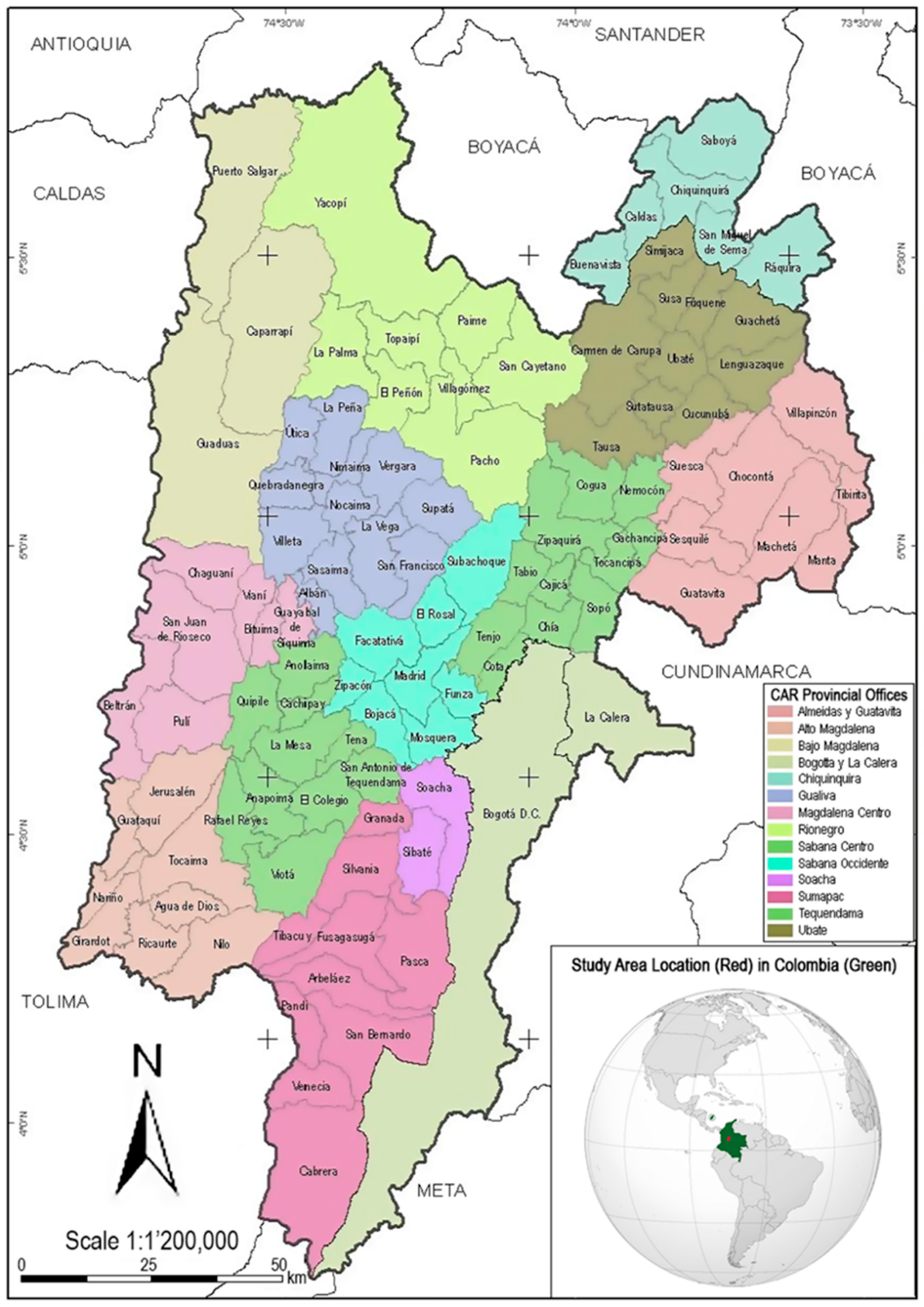
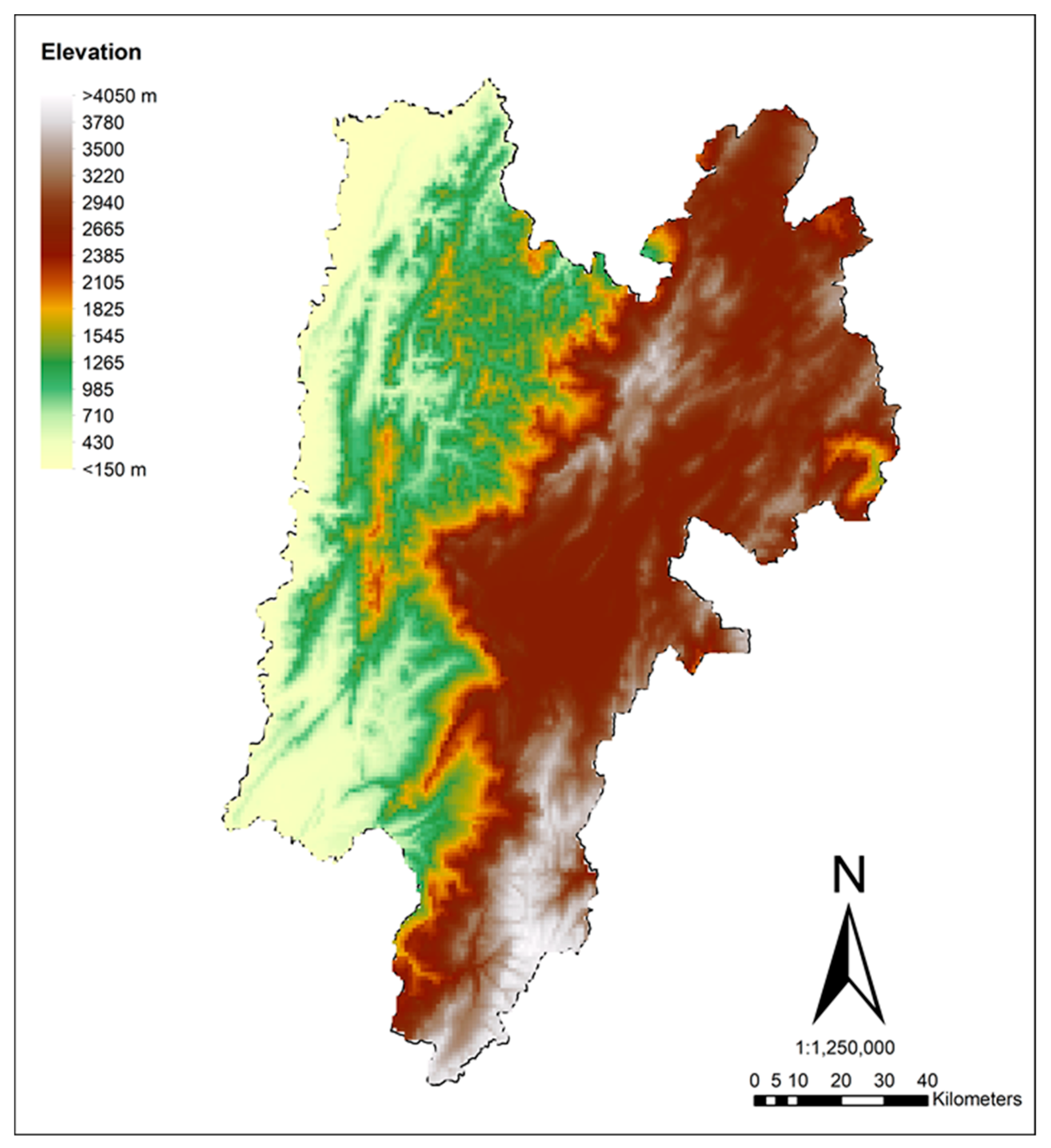
2.1. Characteristics of the Studied Region
2.2. Methods
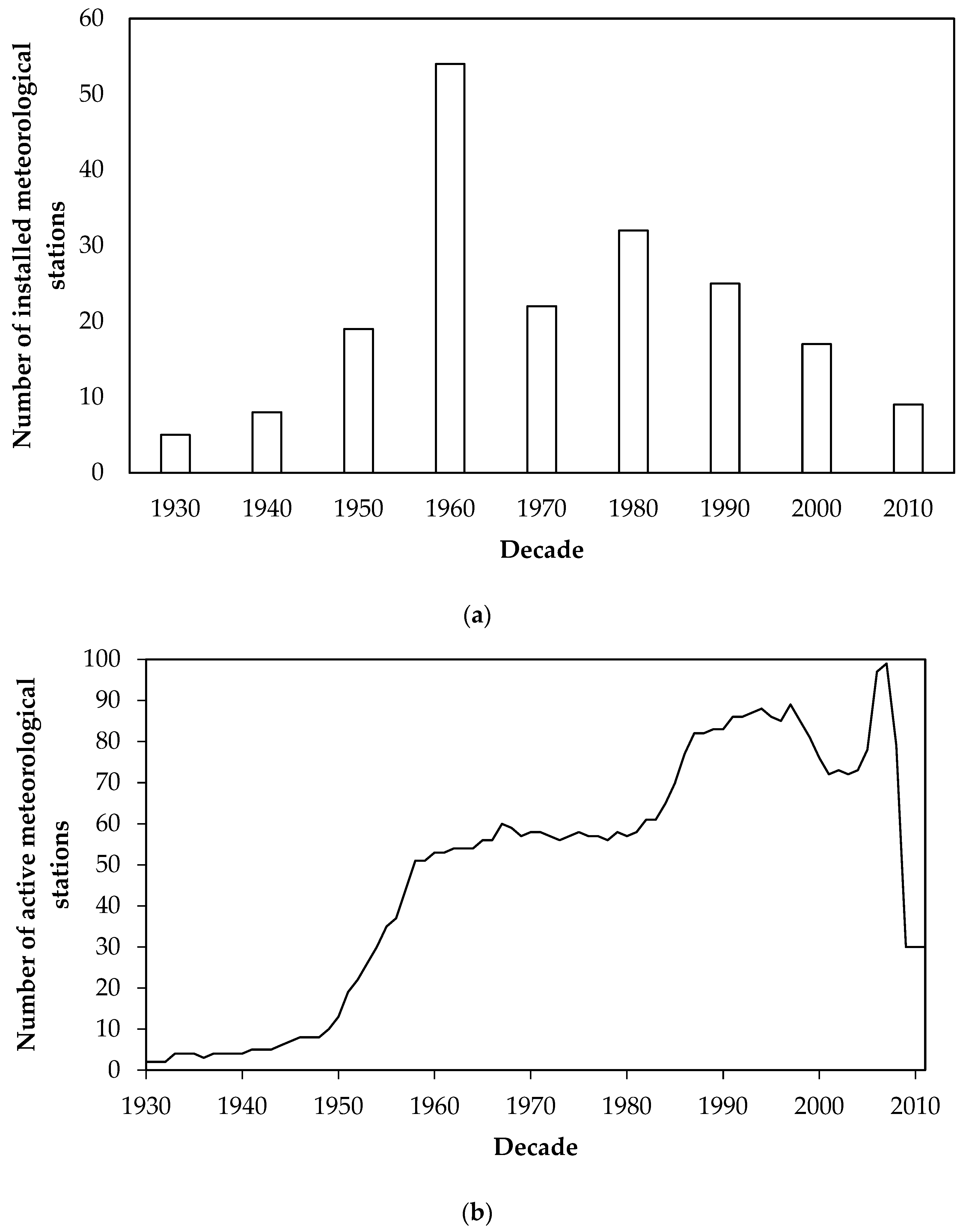
2.2.1. Meteorological Network Data
2.2.2. Data Processing
2.2.3. Development of the Artificial Neural Network Model
2.2.4. Performance Evaluation of the Rainfall Network in the Cundinamarca Region
3. Results and Discussion
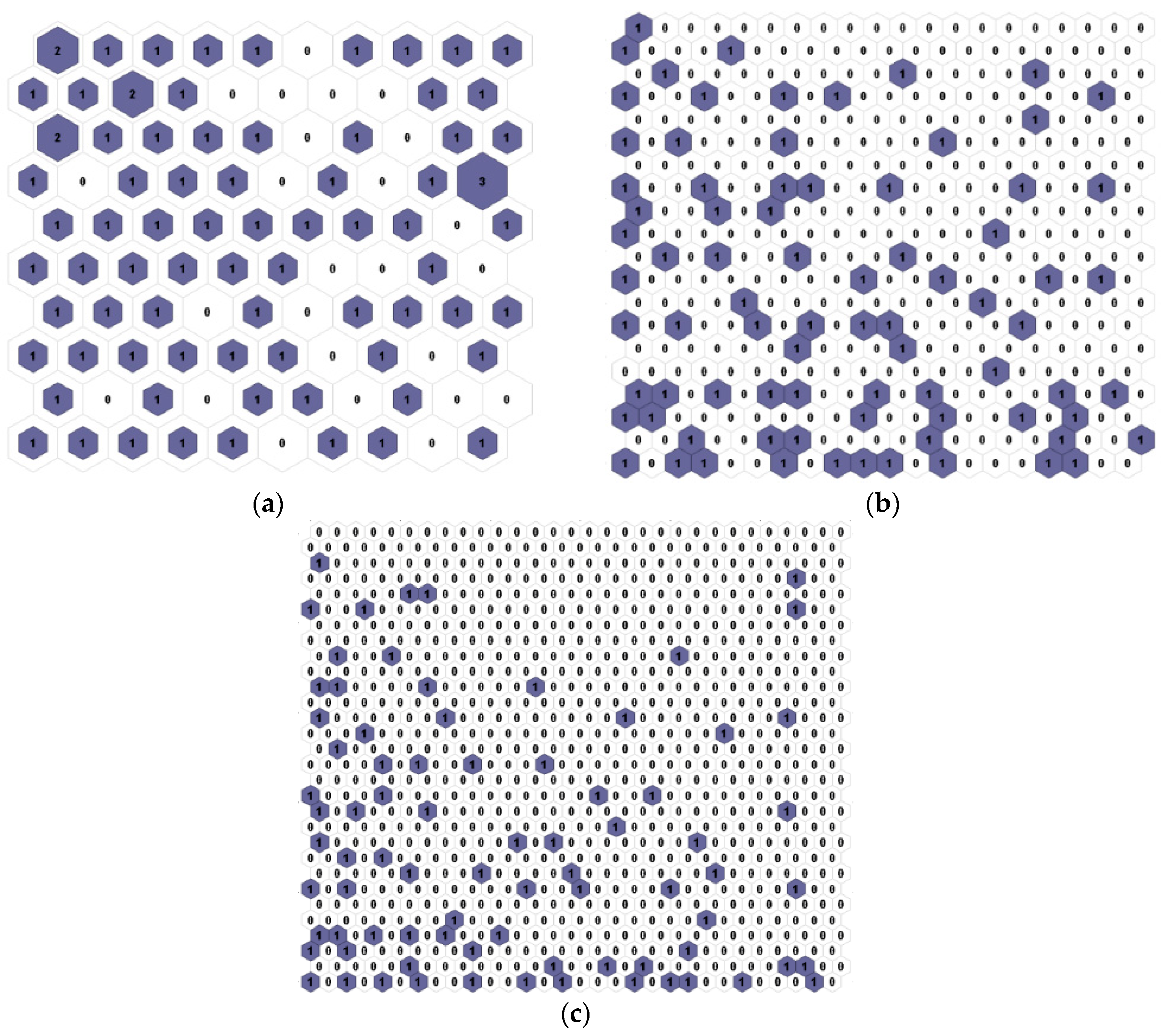
3.1. Classification of Rainfall Stations
3.2. Scenario Configurations
3.3. Mutual Information Classification Analysis
4. Conclusions
Author Contributions
Funding
Acknowledgments
Conflicts of Interest
References
- Zoppou, C. Review of urban storm water models. Environ. Model. Softw. 2001, 16, 195–231. [Google Scholar] [CrossRef]
- Daly, C.; Neilson, R.P.; Phillips, D.L. A statistical-topographic model for mapping climatological precipitation over mountainous terrain. J. Appl. Meteorol. 1994, 33, 140–158. [Google Scholar] [CrossRef]
- Johansson, B.; Chen, D. The influence of wind and topography on precipitation distribution in Sweden: Statistical analysis and modelling. Int. J. Climatol. 2003, 23, 1523–1535. [Google Scholar] [CrossRef]
- Lin, G.F.; Chen, L.H. Identification of homogeneous regions for regional frequency analysis using the self-organizing map. J. Hydrol. 2006, 324, 1–9. [Google Scholar] [CrossRef]
- Rojas-Polanco, M.I.; Mora-Mora, L.E. Optimum design of rainfall network. Rev. For. Venez. 2009, 53, 9–22. [Google Scholar]
- Chowdhury, M.; Alouani, A.; Hossain, F. Comparison of ordinary kriging and artificial neural network for spatial mapping of arsenic contamination of groundwater. Stoch. Environ. Res. Risk Assess. 2010, 24, 1–7. [Google Scholar] [CrossRef]
- Chen, Y.C.; Wei, C.; Yeh, H.C. Rainfall network design using kriging and entropy. Hydrol. Process. 2008, 22, 340–346. [Google Scholar] [CrossRef]
- Karabacak, K.; Cetin, N. Artificial neural networks for controlling wind-PV power systems: A review. Renew. Sustain. Energy Rev. 2014, 29, 804–827. [Google Scholar] [CrossRef]
- Dursun, M.; Özden, S. An efficient improved photovoltaic irrigation system with artificial neural network based modeling of soil moisture distribution—A case study in Turkey. Comput. Electron. Agric. 2014, 102, 120–126. [Google Scholar] [CrossRef]
- Asimakopoulou, F.E.; Tsekouras, G.J.; Gonos, I.F.; Stathopulos, I.A. Estimation of seasonal variation of ground resistance using Artificial Neural Networks. Electr. Power Syst. Res. 2013, 94, 113–121. [Google Scholar] [CrossRef]
- Adib, H.; Haghbakhsh, R.; Saidi, M.; Takassi, M.A.; Sharifi, F.; Koolivand, M.; Rahimpour, M.R.; Keshtkari, S. Modeling and optimization of Fischer-Tropsch synthesis in the presence of Co (III)/Al2O3 catalyst using artificial neural networks and genetic algorithm. J. Nat. Gas Sci. Eng. 2013, 10, 14–24. [Google Scholar] [CrossRef]
- Mohajerani, M.; Mehrvar, M.; Ein-Mozaffari, F. Using an external-loop airlift sonophotoreactor to enhance the biodegradability of aqueous sulfadiazine solution. Sep. Purif. Technol. 2012, 90, 173–181. [Google Scholar] [CrossRef]
- Fukushima, K. Artificial vision by multi-layered neural networks: Neocognitron and its advances. Neural Netw. 2013, 37, 103–119. [Google Scholar] [CrossRef]
- Mallela, U.K.; Upadhyay, A. Buckling load prediction of laminated composite stiffened panels subjected to in-plane shear using artificial neural networks. Thin-Walled Struct. 2016, 102, 158–164. [Google Scholar] [CrossRef]
- Turlapaty, A.C.; Anantharaj, V.G.; Younan, N.H.; Joseph Turk, F. Precipitation data fusion using vector space transformation and artificial neural networks. Pattern Recognit. Lett. 2010, 31, 1184–1200. [Google Scholar] [CrossRef]
- Liu, Q.J.; Shi, Z.H.; Fang, N.F.; Zhu, H.D.; Ai, L. Modeling the daily suspended sediment concentration in a hyperconcentrated river on the Loess Plateau, China, using the Wavelet-ANN approach. Geomorphology 2013, 186, 181–190. [Google Scholar] [CrossRef]
- Garrido-Arévalo, A.R.; Agudelo, L.M.; Obregon, N.; Garrido, V.M. Classification of pluviometric networks located in the region of Bogotá, Colombia using artificial neural networks. J. Phys. Conf. Ser. 2020, 1448. [Google Scholar] [CrossRef]
- Kar, A.K.; Lohani, A.K.; Goel, N.K.; Roy, G.P. Rain gauge network design for flood forecasting using multi-criteria decision analysis and clustering techniques in lower Mahanadi river basin, India. J. Hydrol. Reg. Stud. 2015, 4, 313–332. [Google Scholar] [CrossRef]
- Wei, C.; Yeh, H.C.; Chen, Y.C. Spatiotemporal Scaling Effect on Rainfall Network Design Using Entropy. Entropy 2014, 16, 4626–4647. [Google Scholar] [CrossRef]
- Shannon, C.E. A Mathematical Theory of Communication. Bell Syst. Tech. J. 1948, 27, 379–423. [Google Scholar] [CrossRef]
- Vinod, H.D. Maximum entropy ensembles for time series inference in economics. J. Asian Econ. 2006, 17, 955–978. [Google Scholar] [CrossRef]
- Noonan, J.P.; Basu, P. On estimation error using maximum entropy density estimates. Kybernetes 2007, 36, 52–64. [Google Scholar] [CrossRef]
- Weber, T.C. Maximum entropy modeling of mature hardwood forest distribution in four U.S. states. For. Ecol. Manag. 2011, 261, 779–788. [Google Scholar] [CrossRef]
- Payandeh Najafabadi, A.T.; Hatami, H.; Omidi Najafabadi, M. A maximum-entropy approach to the linear credibility formula. Insur. Math. Econ. 2012, 51, 216–221. [Google Scholar] [CrossRef]
- Aurbacher, J.; Dabbert, S. Generating crop sequences in land-use models using maximum entropy and Markov chains. Agric. Syst. 2011, 104, 470–479. [Google Scholar] [CrossRef]
- Xie, L.; Li, G.; Xiao, M.; Peng, L. Novel classification method for remote sensing images based on information entropy discretization algorithm and vector space model. Comput. Geosci. 2016, 89, 252–259. [Google Scholar] [CrossRef]
- Calisto Acosta, O.E. River gauging with one velocity point based on the principle of maximum entropy. Ing. Hidráulica Mex. 2002, 17, 5–19. [Google Scholar]
- Dalezios, N.R.; Tyraskis, P.A. Maximum entropy spectra for regional precipitation analysis and forecasting. J. Hydrol. 1989, 109, 25–42. [Google Scholar] [CrossRef]
- Mishra, A.K.; Özger, M.; Singh, V.P. An entropy-based investigation into the variability of precipitation. J. Hydrol. 2009, 370, 139–154. [Google Scholar] [CrossRef]
- CAR. 2012–2015 Master Plan; Corporacion Autonoma Regional de Cundinamarca (CAR): Bogota, Colombia, 2012. [Google Scholar]
- Hurtado-Montoya, A.F.; Mesa-Sánchez, Ó.J. Reanalysis of monthly precipitation fields in Colombian territory. DYNA 2014, 81, 251–258. [Google Scholar] [CrossRef]
- CAR. 2016–2019 Master Plan; Corporacion Autonoma Regional de Cundinamarca (CAR): Bogota, Colombia, 2016. [Google Scholar]
- OAS. Manual for Design, Installation, Operation and Maintenance of Systems of Flood Early Warning and Online Database; The Organization of American States (OAS), Department of Sustainable Development: Washington, DC, USA, 2010. [Google Scholar]
- Wang, W.; Wang, D.; Singh, V.P.; Wang, Y.; Wu, J.; Wang, L.; Zou, X.; Liu, J.; Zou, Y.; He, R. Optimization of rainfall networks using information entropy and temporal variability analysis. J. Hydrol. 2018, 559, 136–155. [Google Scholar] [CrossRef]
- CAR. SICLICA—Sistema de Información Climatológica e Hidrológica: Valores Totales Mensuales de Precipitación, Máxima en 24 Horas (mm); Corporacion Autonoma Regional de Cundinamarca (CAR): Bogota, Colombia, 2010. [Google Scholar]
- González-Cuéllar, F.; Obregón-Neira, N. Self-organizing maps of Kohonen as a river clustering tool within the methodology for determining regional ecological flows ELOHA. Ing. Univ. 2013, 17, 311–323. [Google Scholar]
- Hamzehie, M.E.; Fattahi, M.; Najibi, H.; Van der Bruggen, B.; Mazinani, S. Application of artificial neural networks for estimation of solubility of acid gases (H2S and CO2) in 32 commonly ionic liquid and amine solutions. J. Nat. Gas Sci. Eng. 2015, 24, 106–114. [Google Scholar] [CrossRef]
- Lohani, A.K.; Kumar, R.; Singh, R.D. Hydrological time series modeling: A comparison between adaptive neuro-fuzzy, neural network and autoregressive techniques. J. Hydrol. 2012, 442, 23–35. [Google Scholar] [CrossRef]
- Chang, T.K.; Talei, A.; Alaghmand, S.; Ooi, M.P.L. Choice of rainfall inputs for event-based rainfall-runoff modeling in a catchment with multiple rainfall stations using data-driven techniques. J. Hydrol. 2017, 545, 100–108. [Google Scholar] [CrossRef]
- González-álvarez, A.; Viloria-Marimón, O.M.; Coronado-Hernández, O.E.; Vélez-Pereira, A.M.; Tesfagiorgis, K.; Coronado-Hernández, J.R. Isohyetal maps of daily maximum rainfall for different return periods for the Colombian Caribbean Region. Water 2019, 11, 358. [Google Scholar] [CrossRef]
- Elshorbagy, A.; Corzo, G.; Srinivasulu, S.; Solomatine, D.P. Experimental investigation of the predictive capabilities of data driven modeling techniques in hydrology—Part 1: Concepts and methodology. Hydrol. Earth Syst. Sci. 2010, 14, 1931–1941. [Google Scholar] [CrossRef]
- Farsadnia, F.; Rostami Kamrood, M.; Moghaddam Nia, A.; Modarres, R.; Bray, M.T.; Han, D.; Sadatinejad, J. Identification of homogeneous regions for regionalization of watersheds by two-level self-organizing feature maps. J. Hydrol. 2014, 509, 387–397. [Google Scholar] [CrossRef]


| Watershed | Area (km2) |
|---|---|
| Sumapaz River | 2527 |
| Bogota River | 5671 |
| Magdalena River | 2191 |
| Negro River | 4239 |
| Minero River | 990.8 |
| Ubate-Suarez River | 1965 |
| Blanco River | 471.0 |
| Gachetá River | 97.30 |
| Machetá River | 508.7 |
| Input Variable | Transformation |
|---|---|
| Latitude (m) | y = (x − xmin)/(xmax − xmin) |
| Longitude (m) | y = (x − xmin)/(xmax − xmin) |
| Elevation (m) | y = x/xmax |
| Annual rainfall (mm) | y = x/xmax |
| Standard deviation of annual rainfall (mm) | y = x/xmax |
| Monthly rainfall (mm) | y = x/xmax |
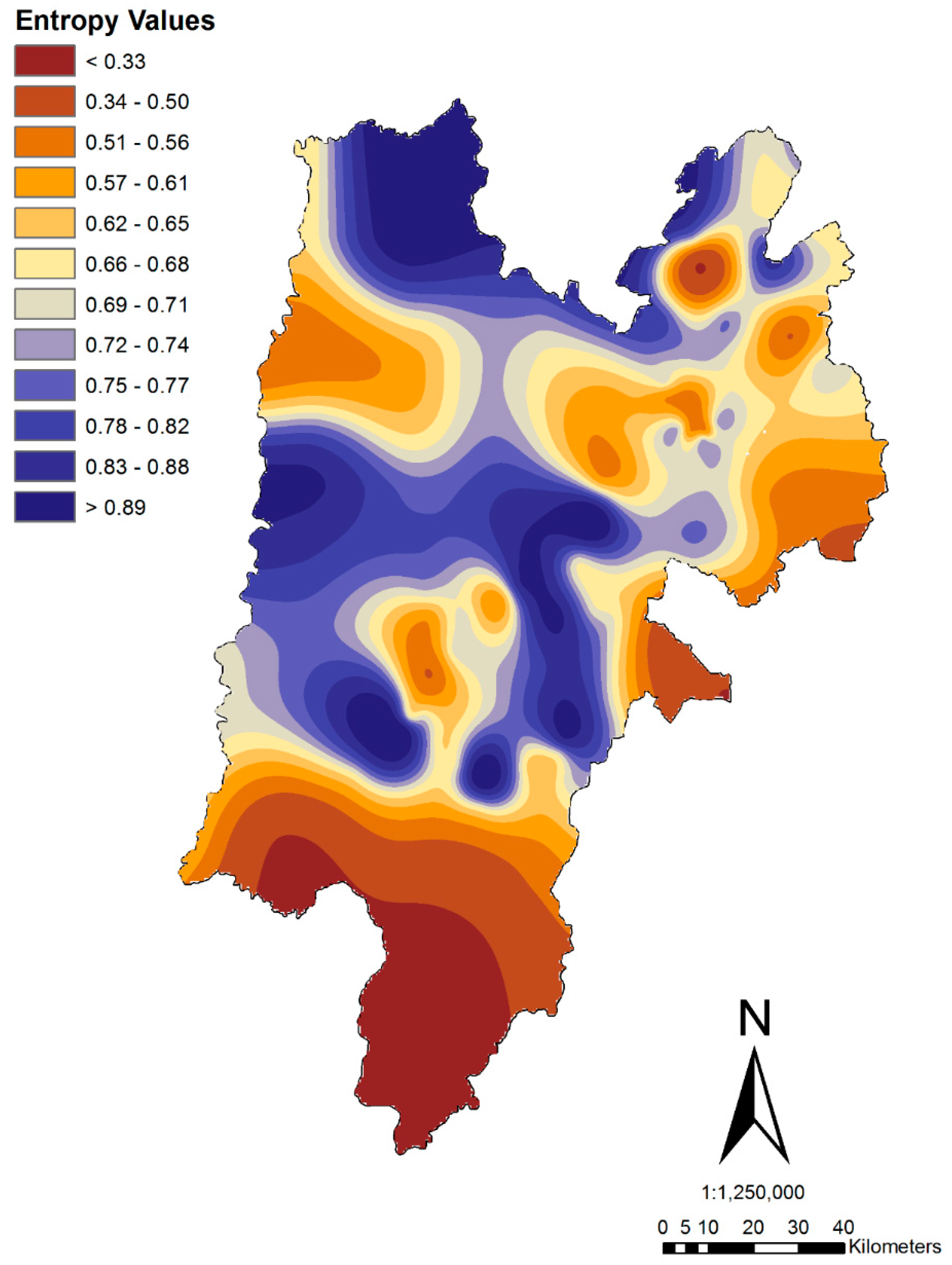
| Mutual Information Range | Index |
|---|---|
| 0–0.5 | High deficit |
| 0.5–1.0 | Deficit |
| 1.0–1.5 | Acceptable |
| 1.5–2.0 | Above average |
| >2.0 | Excess |
| Parameter | Rainfall Station Number | ||||||||||
|---|---|---|---|---|---|---|---|---|---|---|---|
| S1 | S4 | S8 | S9 | S10 | S13 | S15 | S16 | S18 | S22 | ||
| Longitude | 0.6582 | 0.1046 | 0.1765 | 0.6240 | 0.3406 | 0.4603 | 0.9768 | 0.7852 | 0.6414 | 0.4045 | |
| Latitude | 0.4806 | 0.0256 | 0.1008 | 0.5132 | 0.3561 | 0.3755 | 0.6668 | 0.7215 | 0.3214 | 0.3260 | |
| Elevation | 0.7636 | 0.1150 | 0.1093 | 0.8806 | 0.7688 | 0.7837 | 0.8053 | 0.9002 | 0.7417 | 0.7506 | |
| Average monthly rainfall | January | 0.3197 | 0.4796 | 0.5404 | 0.2984 | 0.4240 | 0.3530 | 0.3445 | 0.2358 | 0.5877 | 0.3984 |
| February | 0.3681 | 0.5415 | 0.5799 | 0.3155 | 0.4837 | 0.4429 | 0.3097 | 0.2851 | 0.5078 | 0.5936 | |
| March | 0.3438 | 0.5556 | 0.5726 | 0.4048 | 0.4610 | 0.4513 | 0.3644 | 0.3543 | 0.4520 | 0.5175 | |
| April | 0.2817 | 0.4985 | 0.4060 | 0.2883 | 0.2691 | 0.3447 | 0.2279 | 0.2684 | 0.3012 | 0.3315 | |
| May | 0.3257 | 0.5299 | 0.4270 | 0.3777 | 0.2608 | 0.3329 | 0.4092 | 0.2680 | 0.2975 | 0.3670 | |
| June | 0.3446 | 0.2578 | 0.2759 | 0.4483 | 0.2356 | 0.3174 | 0.5403 | 0.2651 | 0.3430 | 0.4590 | |
| July | 0.4423 | 0.1983 | 0.2441 | 0.5927 | 0.2765 | 0.3589 | 0.6043 | 0.3653 | 0.4742 | 0.5490 | |
| August | 0.2833 | 0.1837 | 0.2197 | 0.5957 | 0.2626 | 0.3128 | 0.4148 | 0.2476 | 0.3009 | 0.4912 | |
| September | 0.3041 | 0.4688 | 0.4408 | 0.3927 | 0.3009 | 0.3613 | 0.3561 | 0.2203 | 0.3655 | 0.4860 | |
| October | 0.4040 | 0.3501 | 0.3811 | 0.3445 | 0.3192 | 0.3827 | 0.3469 | 0.3007 | 0.3461 | 0.4283 | |
| November | 0.2871 | 0.3532 | 0.4962 | 0.3086 | 0.3615 | 0.3209 | 0.2984 | 0.2276 | 0.3648 | 0.3564 | |
| December | 0.2593 | 0.3984 | 0.4038 | 0.2600 | 0.3633 | 0.4133 | 0.3635 | 0.3224 | 0.3810 | 0.4007 | |
| Annual rainfall | 0.3286 | 0.4104 | 0.4169 | 0.3749 | 0.3246 | 0.3627 | 0.3683 | 0.2782 | 0.3720 | 0.4310 | |
| Standard deviation of annual rainfall | 0.3377 | 0.5635 | 0.4935 | 0.3289 | 0.3004 | 0.3365 | 0.3209 | 0.2699 | 0.2519 | 0.3057 | |
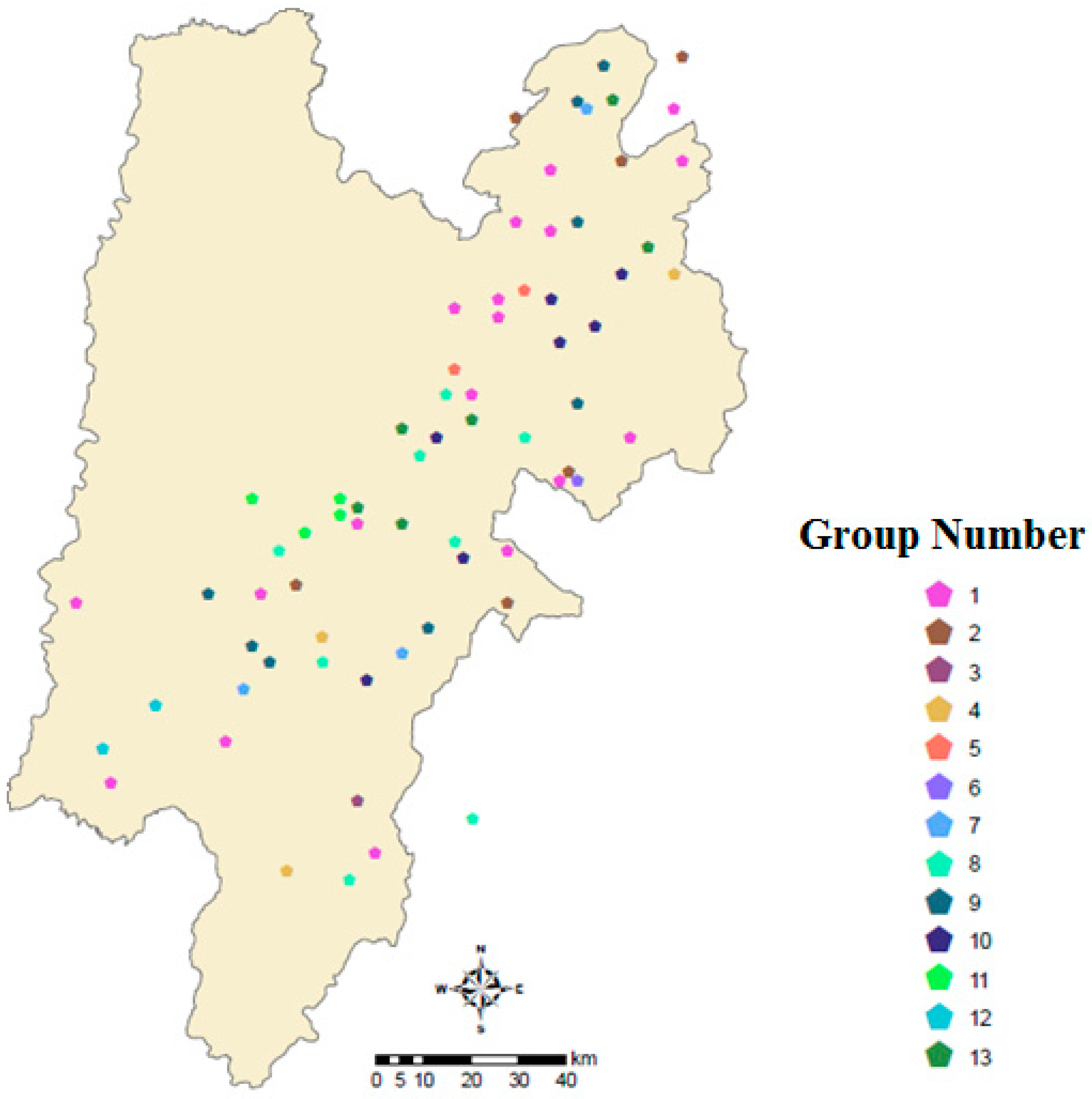
| Group Number | Station List | Number of Grouped Stations |
|---|---|---|
| 1 | S16, S25, S27, S36, S37, S52, S60, S61, S65, S71, S86, S89, S101, S102, S126, S138, S144, S149, S150, S156, S166 | 21 |
| 2 | S29, S31, S40, S76, S96, S122, S158 | 7 |
| 3 | S140 | 1 |
| 4 | S15, S91, S105, S118, S131 | 5 |
| 5 | S85, S97, S109 | 3 |
| 6 | S80 | 1 |
| 7 | S63, S88, S123 | 3 |
| 8 | S9, S18, S28, S41, S45, S108, S142, S151, S174 | 9 |
| 9 | S44, S64, S77, S78, S124, S130, S159, S163 | 8 |
| 10 | S32, S42, S62, S67, S116, S129, S147, S154, S162 | 9 |
| 11 | S10, S13, S22, S81 | 4 |
| 12 | S4, S8, S55 | 3 |
| 13 | S1, S33, S49, S53, S54, S161 | 6 |
© 2020 by the authors. Licensee MDPI, Basel, Switzerland. This article is an open access article distributed under the terms and conditions of the Creative Commons Attribution (CC BY) license (http://creativecommons.org/licenses/by/4.0/).
Share and Cite
Garrido-Arévalo, A.R.; Agudelo-Otálora, L.M.; Obregón-Neira, N.; Garrido-Arévalo, V.; Quiñones-Bolaños, E.E.; Naraei, P.; Mehrvar, M.; Bustillo-Lecompte, C.F. Application of Artificial Neural Network and Information Entropy Theory to Assess Rainfall Station Distribution: A Case Study from Colombia. Water 2020, 12, 1973. https://doi.org/10.3390/w12071973
Garrido-Arévalo AR, Agudelo-Otálora LM, Obregón-Neira N, Garrido-Arévalo V, Quiñones-Bolaños EE, Naraei P, Mehrvar M, Bustillo-Lecompte CF. Application of Artificial Neural Network and Information Entropy Theory to Assess Rainfall Station Distribution: A Case Study from Colombia. Water. 2020; 12(7):1973. https://doi.org/10.3390/w12071973
Chicago/Turabian StyleGarrido-Arévalo, Augusto Rafael, Luis Mauricio Agudelo-Otálora, Nelson Obregón-Neira, Victor Garrido-Arévalo, Edgar Eduardo Quiñones-Bolaños, Parisa Naraei, Mehrab Mehrvar, and Ciro Fernando Bustillo-Lecompte. 2020. "Application of Artificial Neural Network and Information Entropy Theory to Assess Rainfall Station Distribution: A Case Study from Colombia" Water 12, no. 7: 1973. https://doi.org/10.3390/w12071973
APA StyleGarrido-Arévalo, A. R., Agudelo-Otálora, L. M., Obregón-Neira, N., Garrido-Arévalo, V., Quiñones-Bolaños, E. E., Naraei, P., Mehrvar, M., & Bustillo-Lecompte, C. F. (2020). Application of Artificial Neural Network and Information Entropy Theory to Assess Rainfall Station Distribution: A Case Study from Colombia. Water, 12(7), 1973. https://doi.org/10.3390/w12071973