Article

Improvement of SCS-CN Initial Abstraction Coefficient in the Czech Republic: A Study of Five Catchments

1
T. G. Masaryk Water Research Institute, Podbabská 30, 160 00 Praha, Czech Republic
2
Department of Geography, Faculty of Science, Masaryk University, Kotlářská 2, 611 37 Brno, Czech Republic
3
Research Institute for Soil and Water Conservation, Žabovřeská 250, 156 27 Praha, Czech Republic
*
Author to whom correspondence should be addressed.
Water 2020, 12(7), 1964; https://doi.org/10.3390/w12071964
Submission received: 19 May 2020 / Revised: 2 July 2020 / Accepted: 3 July 2020 / Published: 10 July 2020

Abstract

:
The SCS-CN method is a globally known procedure used primarily for direct-runoff estimates. It also is integrated in many modelling applications. However, the method was developed in specific geographical conditions, often making its universal applicability problematic. This study aims to determine appropriate values of initial abstraction coefficients λ and curve numbers (CNs), based on measured data in five experimental catchments in the Czech Republic, well representing the physiographic conditions in Central Europe, to improve direct-runoff estimates. Captured rainfall-runoff events were split into calibration and validation datasets. The calibration dataset was analysed by applying three approaches: (1) Modifying λ, both discrete and interpolated, using the tabulated CN values; (2) event analysis based on accumulated rainfall depth at the moment runoff starts to form; and (3) model fitting, an iterative procedure, to search for a pair of λ, S (CN, respectively). To assess individual rainfall characteristics’ possible influence, a principal component analysis and cluster analysis were conducted. The results indicate that the CN method in its traditional arrangement is not very applicable in the five experimental catchments and demands corresponding modifications to determine λ and CN (or S, respectively). Both λ and CN should be viewed as flexible, catchment-dependent (regional) parameters, rather than fixed values. The acquired findings show the need for a systematic yet site-specific revision of the traditional CN method, which may help to improve the accuracy of CN-based rainfall-runoff modelling.

1. Introduction

The Soil Conservation Service Curve Number (SCS-CN) method is an empirical lumped rainfall-runoff model developed in 1954 by the US Department of Agriculture’s Soil Conservation Service (USDA SCS, now the Natural Resources Conservation Service NRCS). Originally, the method entailed converting basic descriptive inputs characterising catchment features into numeric values of curve numbers (CNs) [1]. For any given rainfall amount, the corresponding runoff level is estimated. The procedure is based on a combination of the water-balance equation
P = I a + F + Q ,
and two fundamental assumptions,
Q P I a = F S ,
  I a = λ S  
in which Q is direct runoff (mm); P is precipitation (mm); Ia is initial abstraction (mm) that has to be exceeded so that direct runoff can start to form; F is cumulative infiltration (mm), not including Ia; S is maximum potential retention of a watershed after the start of the runoff and λ is initial abstraction ratio (dimensionless).
The runoff depth Q is expressed using Equations (1)–(3) as
Q = ( P λ S ) 2 ( P + ( 1 λ ) S   for   P   >   I a ,   Q = 0   for   P     I a .
The maximum potential retention S is expressed as a function
S = 25400 C N 254 ,
in which CN is the curve number, theoretically ranging between 0 and 100. Over the years, the method has undergone numerous modifications [2,3,4,5,6], during which time the scientific community adopted the method globally for its simplicity, applicability and relatively low demands on input data [7,8,9,10,11].
The CN method has various shortcomings regarding practical applications in different geographical conditions. For example, the initial abstraction coefficient λ’s validity has been questioned [11,12,13,14]. Similarly, the role of a watershed’s relief and land cover [15,16,17,18,19,20], previous rainfall’s influence [19,20,21] and CN values’ representativeness [16,22,23] in terms of properly setting the method have been scrutinised.
Attention has been payed to the ability of a single CN value to characterise the runoff response of a watershed correctly. While the CN may be calculated from observed P-Q data, practical experience shows that the CN values vary between events [11,24]. Therefore, various approaches were introduced aiming to estimate an appropriate single CN value or single asymptotic CN, separately [1,25,26,27,28,29]. However, the aforementioned methods showed certain shortcomings addressed by a study that analysed the effect of soil and land cover complexes on the hydrologic responses in watersheds [30]. Specifically, the authors proposed a concept of a two-CN heterogenous system. This study was subsequently generalised [31]. The latter two methods along with other CN estimation methods were used and compared in a study [32] of a watershed affected by a major forest fire, so that the effect of both spatial heterogeneity in land cover and the fire could be investigated.
Another problematic aspect of the CN method lies in the characterisation of previous rainfall. It is expressed using three antecedent moisture condition (AMC) classes (I: Dry; II: Normal; and III: Wet), each of which has its own set of CNs. The discrete character of the CN-AMC relationship is manifested by sudden jumps in estimated runoff [33]. On the basis of previous five-day rainfall totals, CNII is converted to CNI and CNIII using relationships proposed by [24,25,26,27,28,29,30,31,32,33,34,35,36,37] and directly from the NEH-4 tables [4,38,39]. Despite the existence of different conversion methods, the discontinuity problem remained unresolved, and the concept of soil moisture accounting (SMA) became a subject of research. Williams and LaSeur [40] presented the first SMA concept. Their procedure was based on the idea that the CN varies continuously, along with soil moisture. Hawkins [41] then developed a continuous soil moisture accounting concept, but this modification did not take into account the SCS-CN procedure’s structural shortcomings in terms of SMA, a problem addressed by Mishra et al. [42], who introduced an improved SMA-based SCS-CN model. Subsequently, Mishra and Singh [43] developed a versatile SCS-CN model (VSCS-CN) based on the assumption that higher antecedent soil moisture before a rainfall event will provide greater runoff and lower the soil’s capacity to store and retain rainfall water. Similarly, Michel et al. [44] also examined such a concept. Mishra and Singh [21] used a concept that comprised a runoff coefficient and the degree of saturation on the basis of which multiple improved SCS-CN models have been proposed [19,45,46,47,48,49].
Relief is a significant factor in runoff formation [50,51], but slope was not reflected in the traditional CN model. The NRCS handbook’s CN values [6] are viewed as corresponding to a 5% slope [18,20,51,52]. However, some approaches exist that incorporate slope into the CN estimates. For example, Huang et al. [51] modified the procedure by Sharpley and Williams [18] for steep watersheds in Loess Plateau, China. Their method then was adjusted for rainfall-runoff data from 39 South Korean watersheds. However, according to Mishra et al. [8], the aforementioned procedures require proper validation.
Inaccuracies in direct-runoff modelling are frequently associated with the initial abstraction Ia or λ, separately. Ia was not incorporated into the original CN method [52]. During its evolution, a constant value of 0.2 was set for λ [4,53], but many authors challenged this. Trying to identify this constant’s appropriate value has been a matter of many debates and studies conducted to estimate the appropriate value of λ. It was concluded by several studies that λ values result from multiple factors related to rainfall events and landscape features [22,54,55] and that the coefficient should be viewed as a regional parameter expressing geographical variability [10]. Some researchers concluded stated that λ can take any non-negative value, in some cases even greater than 1 [55,56,57,58,59]. However, many authors stated that using reduced λ led to much more accurate results, e.g., [2,11,12,13,60,61,62,63,64].
In the Czech Republic, the CN method is applied frequently, using tabulated CN values [65]. The value of λ implicitly is set at 0.2, but such a value does not appear to be representative, as preliminary studies by Caletka and Honek [66] and Caletka and Michalková [67] concluded. The CN method is the subject of greater interest in Slovakia where several studies were conducted in recent years. Karabová [68] analysed rainfall-runoff data from five lowland watersheds in Slovakia, addressing the problem of regionalisation of runoff curve through a new AMC classification and application of λ–P regressions. The study concluded that the traditional CN method lead to over-estimated direct runoff for lower P and vice versa. Similarly, Kohnová et al. [69] analysed rainfall-runoff data from nine watersheds in central Slovakia and concluded that the standard CN method demanded certain modifications. Specifically, they stated that CNs should be estimated on the basis of observed rainfall-runoff data, rather than using tabulated values. Moreover, they used the variable λ value instead of the fixed one. Another study [23] compared the original CN method’s performance with that based on empirical rainfall-runoff events using different approaches. They stated that the CN method was burdened by a lot of uncertainty. Using asymptotic fitting procedure of median procedure with reduced λ = 0.05 increased the accuracy of the results. Recently, Kohnová et al. [70] proposed and evaluated the performance of a regionally based approach to estimate CN along with different λ values. They collected data in a group of Slovak and Polish catchments and used the L-moment based method and ANOVA for delineation of two homogenous regions of catchments with similar CNs. The optimal value of λ was set to 0.15.
Given that the application of the CN method in its original form is problematic, based on findings in many studies, this research focuses on an analysis of recorded rainfall-runoff data from five experimental watersheds in the Czech Republic with various geomorphological and agricultural conditions. This study’s main objectives are: (1) To calculate adjusted λ both as discrete values and regression functions; (2) to compare the CN method’s performance using adjusted λ values; and (3) to test the application of the modified CN method in HEC-HMS simulations of specific rainfall-runoff events in a chosen catchment.

2. Study Area

The study was carried out in five experimental watersheds in the Czech Republic (Figure 1), differing mainly in size and in land use. This made it possible to assess the CN method’s performance and interpret the findings of this research with regard to each watershed’s specific geographical conditions. All the studied watersheds’ basic characteristics are provided in Table 1.

2.1. Husí Creek Catchment (FU)

Husí Creek is a left-side tributary of the Oder (Odra) River, located in northeastern Czech Republic, approximately 30 km southwest of the city of Ostrava. The upper parts belong to the easternmost edge of the Bohemian Massif in the Nízký Jeseník Highlands, while the lower parts lie in the Outer Subcarpathia, a depression at the outer base of the Carpathian arc. The catchment’s position predetermines its specific relief; it is characterised by a flat or slightly wavy surface in the upper parts that gradually passes into narrowing valleys with greater longitudinal slope. The valleys widen downstream, and the surface becomes slightly curved to flat. Two main soil types are present in the catchment. Cambisols are found mainly in the upper parts, while luvisols are prevalent in the lower parts. As for land use, a specific spatial distribution exists. Arable land, usually in the form of large plots, is found both in the upper and lower parts of the catchment on the flat relief. Forests and meadows are located mostly in the transition between the upper and lower parts, in the valleys and along streams. This specific environment creates favourable conditions for generating flash floods from intense rainfall. Two major flash-flood events were recorded in summer 2009 and 2010 [71,72]. On 2 July 2009, the region experienced extreme rainfall (local precipitation reached up to 50 mm) after a very rainy period, causing a severe flood event with peak discharge of 33.1 m3/s and corresponding to a 50-year flood event. On 1 June 2010, another rainfall event was recorded (with a maximum rain-gauge measurement of 55 mm), but due to the precipitation’s differing spatial distributions and lower previous rainfall, peak discharge reached only 14.4 m3/s, corresponding to the return period of 5–10 years. Nevertheless, both events resulted in heavy damage to municipalities along the stream.

2.2. Suchý Creek Catchment (NE)

The study area is located approximately 30 km north of Brno in the Drahany Highlands. The catchment is drained by a minor stream, Suchý Creek, and forests cover the western part of the watershed. More than half the area is arable land. Due to large fields, soil erosion poses an imminent threat to a little dam that was constructed right under the catchment’s outlet to protect the areas downstream from flash floods [73].

2.3. Kopaninský Creek Catchment (KO)

This catchment is located in the Křemešnice Highlands in the southern part of the Sázava River basin, a right-side tributary of the Moldau (Vltava) River. It is a source of drinking water for the City of Prague, located approximately 80 km to the northwest. From a geological perspective, this is a very old area formed by igneous and metamorphic rocks during the Paleozoic Era, including granite and schist. Rolling hills and low mountains dominate this region’s surface, with the altitude mostly ranging between 500 and 650 m. As for the soils, cambisols are found most frequently here, along with pseudogleys and gleys, in valleys and along streams. The landscape is covered predominantly by arable land, forests and, to a lesser extent, grasslands and meadows. The settlement is scattered in rather small villages.
The KO catchment is drained by the Kopaninský Creek. The main catchment outlet is KO-3, another two sub-catchments analysed in this study are KO-2 and KO-1. The KO-2 catchment is located in the uppermost part of the KO-3 catchment and has the greatest portion of forested areas, at more than 44%. The KO-1 catchment, located in the lower part, is covered almost entirely by arable land (more than 97%) and is partly tile-drained.
All five studied watersheds’ basic geographical characteristics are listed in Table 1.

3. Materials and Methods

3.1. Data Collection

Automatic rain gauges were used to measure precipitation heights. The monitoring network included up to 17 rain gauges (automatic 0.2 mm tipping buckets 200 cm2 and 0.1 tipping buckets 500 cm2) in catchment FU and its nearby surroundings. The Thiessen polygon interpolation procedure was used to calculate average precipitation levels [74]. A single rain gauge (automatic 0.2 mm tipping bucket 200 cm2) was used to measure rainfall in catchments NE and KO. Using the precipitation data, individual rainfall events were identified, for which five- and 10-day antecedent precipitation totals (P5d, P10d) were calculated.
The water level data were measured using calibrated weirs with ultrasound probes (Fiedler company)—a Thompson weir was used with in catchments NE, KO-1 and KO-2, a compound Cipolletti weir was used in catchment KO-3. In catchment FU, water levels were measured using hydrostatic level sensors (Fiedler company). Discharge values were calculated by means of rating curves set for all monitored outlets on the basis of hydrometric measurements, levelling and using the Chézy formula [75].
An overview of measuring devices is provided in Table 2.

3.2. Estimate of CN Values

The hydrologic soil groups (HSGs) were derived based on Valuated Soil-Ecological Units (VSEUs), a whole-country database (1:5000) determined by the Research Institute for Soil and Water Conservation (RISWC). Land-cover units were identified based on aerial images and a reconnaissance field survey. The corresponding percentages are provided in Table 1, and the spatial distribution is depicted in Figure 2. Moreover, cropping and tillage history also was considered in the NE catchment. Subsequently, the final identification of CNs for each unit was done according to Janeček et al.’s [56] methodology, which frequently is applied in the Czech Republic, in which the tabulated CN values correspond to different HSGs, land-use units and crop types. Moreover, moisture conditions are reflected through antecedent moisture conditions (AMCs). AMCs are characterised by three degrees (I: Dry; II: Normal; and III: Wet), delimited by a five-day precipitation total of P5d of 36 mm and 53 mm prior to a rainfall (P5d < 36 mm—dry conditions; P5d ≥ 53 mm—wet conditions). Maps of CNII values are provided in Figure 2 for each catchment.

3.3. Events, Determination of λ

To avoid biased λ values, rainfall events recorded between April and September with P ≥ 5 mm were chosen for the analysis. In order to exclude rainfall events that caused compound hydrographs, rainfall-runoff events were selected individually, so that the influence of runoff from previous rainfall events could be obviated. For each event, the following parameters were determined:
  • precipitation level P (mm),
  • rainfall event’s duration (h),
  • maximum rain intensity imax (mm h−1),
  • five- and 10-day rainfall accumulations P5d and P10d (mm),
  • hydrograph was drawn and base flow was separated from the hydrograph based on the hydrograph’s inflection points, which indicated the start of the rising limb and the end of the recession limb for each runoff event [69,70],
  • direct-runoff level Q was calculated (mm),
  • initial abstraction Ia (mm), which was calculated as the rainfall level at the moment when direct runoff begins. Such a procedure has been used for instance in research by Shi et al. [11]. However, in large watersheds and/or in case of uneven spatial distribution of precipitation such a calculation of Ia might be problematic as the runoff needs some time to reach the watershed’s outlet [24].
The aforementioned parameters were applied in the analyses described in detail in the following sections. To verify the adjusted CN method’s performance, events’ datasets were split into training and validating datasets (see the numbers provided in Table 2), so that they were similar in terms of level and variability of P, P5d and P10d.

3.3.1. Principal Component Analysis, Cluster Analysis

In order to reveal possible concealed relationships between parameters of rainfall-runoff events and to assess objectively the role that the individual parameters may play in the rainfall-runoff process, principal component analysis (PCA) and cluster analysis (Ward’s method) were conducted for the training datasets from all experimental catchments. The cluster analysis allowed to explore groups (clusters), which the events tend to form. The optimal number of clusters was set using Pham et al.’s [76] k-selection method.

3.3.2. Modified λ with Tabulated CNs

The procedure begins with the determination of tabulated CN values [65] for individual units in a catchment following the procedure described in Section 3.2. For each unit, from the CN values, maximal potential retention S values are derived using Equation (5). Average S for the entire watershed area is calculated using weighted arithmetic mean. In the following step, the corresponding initial abstraction coefficient is calculated using Equation (4), which is converted into the quadratic formula
( S 2 ) λ 2 + ( 2 P S Q S ) λ + ( Q P + Q S P 2 ) = 0 ,
producing a pair of initial abstraction coefficient values for each event. From these, the final selection is carried out following the assumption that the lowest nonnegative value must be chosen. Numerically, the solution of the quadratic equation is correct. However, initial abstraction coefficient λ must be higher than or equal to zero. In case of two non-negative roots, choosing the higher one causes initial abstraction Ia being too high, resulting in zero direct runoff generated as the condition from Equation (4) is not met.
The determination of S values and subsequent calculation (Equation [6]) were conducted twice: (1) Taking into consideration the AMC classes (i.e., using CNI, CNII and CNIII); and (2) neglecting AMC classes and using only CNII, assuming that the AMC determination might not be a deciding factor in calculating direct runoff.

Discrete λ

This procedure’s objective was to identify a discrete representative λ for a watershed calculated as mean and median of values obtained using Equation (6). Mean and median λ were calculated for the entire training dataset of events and for clusters delimited by the cluster analysis.

Interpolated λ

This procedure’s objective was to express λ as a linear function of P [66], instead of using a single value. The regression equations were derived using λ:P plots. Again, the calculations were carried out with and without determination of AMC.

3.3.3. λ Modifications Not Dependent on Tabulated CNs

Event Analysis

This procedure was an inverted process. The maximum potential retention, S, and λ were calculated on the basis of rainfall and runoff parameters. The calculation included the following steps:
  • The total runoff Q and the initial abstraction Ia were calculated using the procedures described above (Section 3.3).
  • The maximum potential retention, S, was an unknown parameter that was calculated using equation
S = ( P I a ) 2 Q ( P I a ) ,
obtained by modifying Equation (4).
3.
The initial abstraction coefficient λ values were determined by dividing Ia by S for each rainfall-runoff event. Mean and median λ were calculated for each experimental watershed.
4.
Regression of S, according to P10d, was calculated and used for the validation together with mean and median λ.

Model Fitting

Model fitting is an iterative least-squares procedure for determining a pair of λ and S such that the sum of the squared differences between the runoff observed and modelled
  [ Q ( P λ S ) 2 ( P + ( 1 λ ) S ) ] 2
as a minimum. The computation of the model-fitting procedure was carried out using a loop-based script in Python 3.7.

3.4. Comparison of Estimated Runoff

For each experimental catchment, a training dataset of events was chosen to identify the key relationships characterising the CN method’s proper setting. The remaining events were used for the parameter validation.
The quality of the runoff levels estimated by the modified CN method was evaluated by means of Nash–Sutcliffe model efficiency coefficient (NSE) (9), and bias (e) (10).
NSE is given as
N S E = 1   ( Q p i Q i ) 2   ( Q i Q a ) 2 ,
in which Qpi is the i-th modelled runoff depth, Qi is the i-th observed runoff depth and Qa is the mean observed runoff depth.
Bias (e) is given as:
e = i = 1 n ( Q p i Q i ) n .
NSE can range from −∞ to 1. An NSE equal to 1 expresses a perfect match of the modelled and observed values. An NSE ≥ 0.5 indicates a very good prediction ability for the model. A lower NSE indicates a worse performance by the simulations. The e is the average difference between the modelled and predicted runoff, thereby expressing the model’s under- or over-estimating tendencies.

3.5. HEC-HMS Simulations

To test the applicability of the modified SCS-CN parameters for simulation of surface runoff, HEC-HMS 4.3 software was used. The simulations’ aim was to verify the model’s ability to deliver a runoff volume/level that did not differ from the observed one by more than 10%, with an NSE ≥ 0.500 (i.e., corresponding to the observed hydrograph’s time course). Such simulations are viewed as sufficiently accurate. The computations were carried out only in the NE catchment, which is relatively small (A = 2.8 km2), thereby allowing for better simulation of the surface runoff and identifying the surface-runoff simulations’ response to changes in individual parameters provided in Table 3.
The catchment was split into three sub-basins. Calibration was carried out for two types of runoff events: (1) Those with a gradual onset, and (2) those with both a rapid onset and rapid recession limb.
The initial abstraction, Ia, was calculated using the curve numbers estimated for the sub-basins through the method described in Section 3.3, the λ values from the original SCS-CN method (λ = 0.2) and the median λ values (λ = 0.0142) from the analysis of which the results are provided in Section 4.2 The percentage of impervious surfaces (buildings and sealed roads) was calculated using ESRI ArcGIS 10.7 software. Time of concentration, Tc, was calculated using Dingman’s [77] formula,
T c = 1.67   3.281   L 0.8 ( 0.0394   A + 1 ) 0.7 1900   Y ,
in which L is the longest flow distance path in a sub-basin (m), A is the sub-basin’s area (km2) and Y is mean slope (%). Dingman’s formula (11) commonly is used in calculations by the Czech Hydrometeorological Institute (CHMI).
The initial discharge at each sub-basin’s outlet was calculated using the main outlet’s value according to the percentage of the sub-basin areas in the entire NE catchment. The remaining parameters (i.e., storage coefficient, recession constant and ratio) were set so that the calibration delivered the best possible result expressed by the bias of the runoff volume/level and NSE. Calibration coefficients were calculated for Ia, CN and Tc as rates of the calibrated values to the original ones. Finally, two sets of these values were available: (1) For the runoff events with slow onset, and (2) for runoff events with rapid onset.
In the subsequent step, two verification events were chosen—one with a slower rising limb and another with rapid onset. Having known the P5d (AMC, respectively), the original CN, Ia and Tc values were used for both λ = 0.2 and λ = 0.0142, corresponding to each verification event’s year. These values were multiplied by the calibration coefficients acquired in the calibration simulations. The storage coefficient, the recession constant and the ratio were calculated in the calibrations.

4. Results

4.1. Influencing Parameters

4.1.1. Principal Component Analysis

To reveal various rainfall and runoff parameters’ influence on runoff response to rainfall at event level, principal component analysis (PCA) and cluster analysis were conducted for the studied watersheds.
The PCA analyses’ outputs are presented in Figure 3. Table 4 provides an overview of the variability percentages that the first two principal components (PC1 and PC2) explain, including all input parameters’ loading values in relation to PC1 and PC2. The variability percentages explained by PC1 and PC2 differ between the studied catchments. In the FU catchment, PC1 showed a value of over 71% and PC2 less than 14%. In the other catchments, PC1 and PC2 percentage differences were not as big. The least difference was recorded in the KO-1 catchment (PC1 49%, PC2 40%). The vectors’ orientation in Figure 3 and the loading values in Table 4 indicate that P10d and P5d present the most influential parameters in the direction of PC1, with maximal rain intensity and P being the most influential parameters in the direction of PC2. The KO-1 catchment has an opposite arrangement, as maximal rain intensity and P have the highest loading values in PC1 and P10d and P5d in PC2. This might be caused by the high percentage of arable land with presence of tile drainage system [78]. In such environment, P10d and P5d do not play the most influential role. Instead, direct runoff formation is dominated by the rain intensity along with P. Higher rain intensity produces faster and higher surface runoff and vice versa. This applies in general, but is probably accentuated in this specific catchment, making it different from the other ones.
To sum up, PCA indicates that P10d and P5d are the most influential parameters. The effects from maximal rain intensity and P, the other two most influential parameters, can be viewed as opposites, as they act along PC2.

4.1.2. Cluster Analysis

Using the methodology introduced by Pham et al. (2005), the optimal number of clusters was determined to be two for the experimental watersheds. Subsequently, non-hierarchical k-means clustering was conducted. Mean and median values of variables in the delimited clusters are listed in Table 5. A difference in P5d and P10d between the delimited clusters in the studied watersheds is apparent. Such a finding corresponds to the output of the cluster analysis. Given that P10d was identified as the most important factor, P10d threshold values were calculated for the catchments to be able to distinguish the cluster to which an event belongs. To determine thresholds, the mean of the upper quartile P10d from the cluster with smaller P10d and the lower quartile P10d from the other cluster (i.e., a cluster with higher P10d) was calculated. The same procedure was applied to calculate the corresponding P5d thresholds, as the P5d normally is used in the traditional SCS-CN procedure to determine AMC classes. The P5d and P10d thresholds were 26 mm and 47 mm in the FU catchment, 18 mm and 39 mm in the NE catchment, 35 mm and 42 mm in the KO-1 catchment, 41 mm and 50 mm in the KO-2 catchment and 20 mm and 28 mm in the KO-3 catchment. For each catchment, these P5d and P10d thresholds were used for separation of rainfall-runoff events into two groups in analyses across the paper.

4.2. Tabulated CN-Based λ Modification

The first way to improve the CN method is through incorporation of tabulated CNs [65] along with modified λ values. The following calculations were carried out with and without taking into consideration the separation of rainfall events according to the P5d and P10d thresholds determined through the cluster analysis. Moreover, AMC classes’ effect was examined by performing the calculations with and without the AMC classification. Modified λ was calculated as a discrete value and as functionally dependent on P.

4.2.1. Discrete λ

For the comparison, the original CN method with λ = 0.2 was applied, and the results showed that in this form, the model mostly was unable to deliver good results, except for the KO-1 catchment (for λ = 0.2 NSE = 0.861). Partial improvements were recorded in simulations with the AMC classification omitted. Only in the KO-1 catchment, the accuracy reduced significantly (NSE dropped from 0.861 to −16.769, see Table 6 and Figure S1a,b). It is important to emphasize that the traditional CN method is limited in terms of “zero runoff” cases since the condition from Equation (4) is often not met due to high λ, and also due to the effect of spatial variability in catchments [30,31], which, however, was not addressed in the present study. The relatively good results for the traditional CN method needs to be confronted with high numbers of events for which the model was unable to deliver non-zero direct runoff. This is apparent in Figure S1a,b. Specifically, the number of non-zero cases ranged from 0 to 13 for simulations with AMC classified and from 7 to 27 for simulations with AMC implicitly set as normal (AMC = II).
To improve the CN method’s performance, mean and median λ values were determined in the training datasets as a whole and in groups separated according to the P5d and P10d thresholds. Generally, the analysis revealed that in most instances λ was lower than 0.2. In the unseparated datasets, mean λ ranged from 0.0365 to 0.1623 and median λ from 0.0142 to 0.0913. Except for one catchment (KO-1), the reduction of λ led to improvements in estimated runoff, since NSE exceeded 0.500, thereby indicating sufficient accuracy. In simulations with separation of events according to P5d and P10d thresholds, a greater variability in λ values existed, ranging from 0.0183 to 0.4231. Despite the expectation that this greater diversification of λ values will lead to more accurate results (in relation to the non-cluster-based approach—all, i.e., without the separation according to P5d and P10d), this assumption only partially was fulfilled. In the FU catchment, the cluster-based approach improved all direct runoff estimates. In the NE catchment, better results were delivered for median. In catchments KO-2 and KO-3, only simulations with median λ applied in events separated according to P10d led to increased accuracy in estimates. No positive response was recorded in simulations using the modified λ values in the KO-1 catchment (NSE ranged from −7.993 to 0.323).
In examining the calculations while not considering AMC classes (AMC implicitly was set to II, normal), higher accuracy in calculated runoff was recorded in the original CN approach, except for the KO-1 catchment. The cluster-based simulations led to better runoff matches only in the FU and NE catchments. In the other catchments, accuracy even decreased significantly.
In summary, the results show that replacing λ originally set to 0.2 with lower values can lead to improvements in direct-runoff simulations. However, the KO-1 catchment was the only one in which no positive effect from the λ modification was recorded. High e values indicated the model’s over-estimating tendency in this specific catchment, probably due to improper CN determination. This might have been caused by the high percentage (97.3%) of arable land along with the presence of the tile drainage systems [78]. In other words, the results revealed quite specific hydrologic conditions in KO-1 catchment compared to the other two KO catchments. Moreover, this well illustrates that CN determination based solely on the prescribed criteria [65] might be misleading. Instead, it should take into consideration all available data on an area of interest.
It should be noted that some studies stated that the modification of λ should be accompanied by a corresponding adjustment in CN or S, separately [2,16]. Therefore, such an approach also was used in this research, but this did not lead to better results than those presented above.

4.2.2. Interpolated λ

Besides discrete values, λ can be expressed as a linear function of P [66,67]. The linear λ–P regressions were calculated for each catchment with and without AMC classification. Analogously to the previous approach (Section 4.2.1), regression equations were calculated for datasets delimited by the P5d and P10d thresholds determined through cluster analysis. All the regression equations are provided in Figure 4 and Table 7.
Generally, application of the λ–P linear regressions increased the runoff estimates’ accuracy. However, for higher Q the estimates showed systematically underestimating tendency (see Figure 5). Moreover, the effect differed between the experimental catchments. In the FU catchment, the best performance (NSE = 0.670) was recorded with using regression for the entire dataset (all-i.e., without the separation according to P5d and P10d). In the other four catchments, the cluster-based regressions (i.e., those considering the separation according to P5d and P10d) delivered the best outputs. However, only in catchments NE and KO-3 did NSE values exceed 0.500 (specifically, 0.670 and 0.540 in the NE catchment, 0.536 and 0.620 in the KO-3 catchment). Applying the all regression in the NE catchment reduced NSE from −0.070 (original CN method) to −0.740. In the KO-3 catchment, the effect was opposite as NSE increased from −26.3 to 0.386. In the remaining catchments KO-1 and KO-2 the results were similar, but NSE values did not indicate sufficient accuracy. Better results were obtained from simulations that omitted the AMC classification in general (see Figure S2), but NSE exceeded 0.500 only in the FU catchment (all regression—NSE = 0.600) and the KO-3 catchment (cluster-based P5d regression—NSE = 0.507).
Compared with the “discrete λ” approach, the regression-based simulation appears to be more stable in terms of overall enhancement of the CN method’s performance. The results indicate that λ should be a variable and event-dependent value. However, the irregular arrangement of the results hints that reliable usage of robust regression-based approach will require a subsequent detailed research of more rainfall-runoff data from various watersheds.

4.3. Approaches Not Dependent on Tabulated CNs

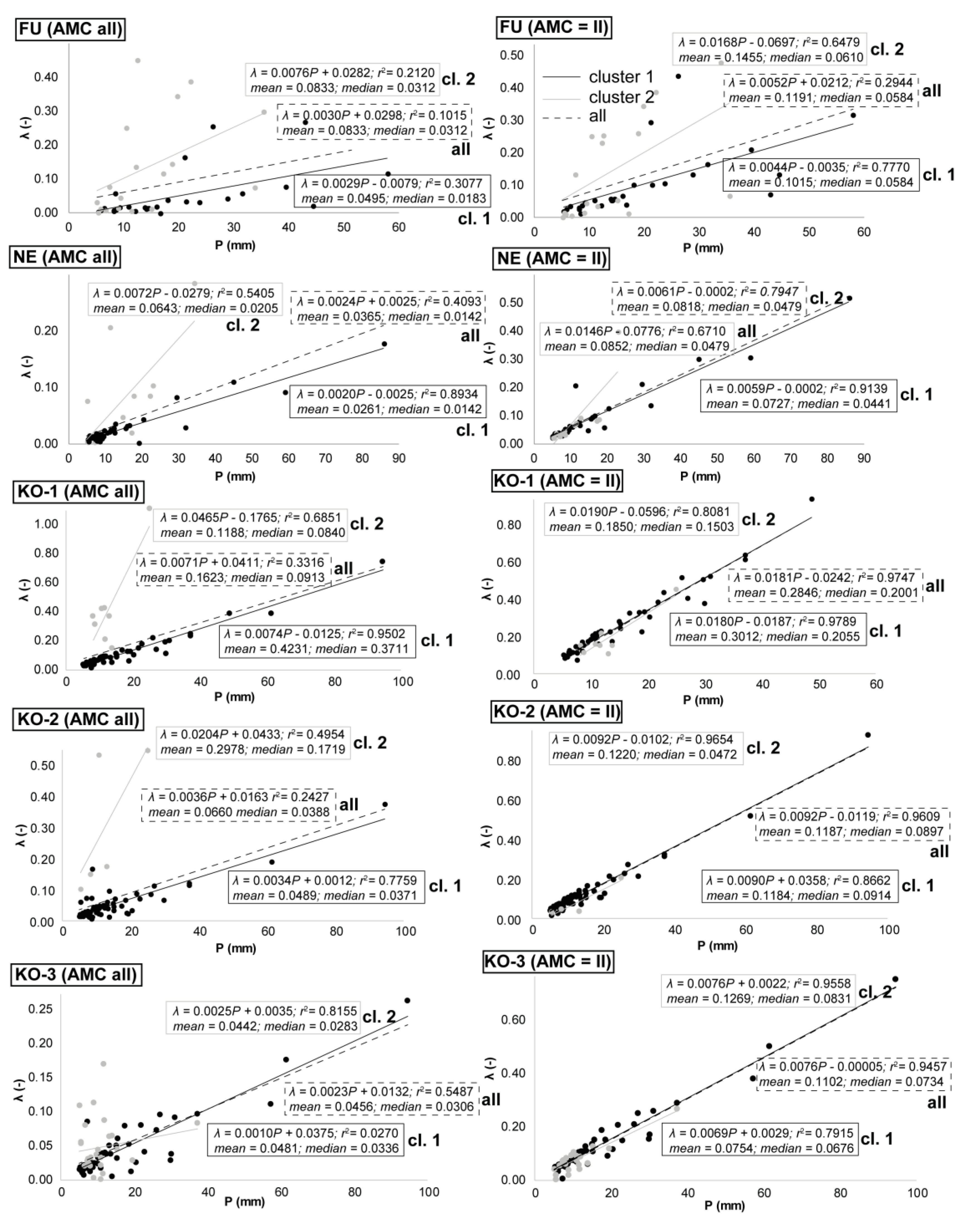
4.3.1. Event Analysis

Unlike the previous analyses, this approach does not start with determining CNs in the watersheds. Instead, it is based on analysing the rainfall-runoff events’ parameters (P, Ia, Q), from which λ and S are derived. This procedure aims to analyse the array of λ and S to reveal a natural relation between them. PCA revealed that P10d poses the most important variable in the arrangement of events (see Figure 3). Therefore, regressions for S according to P10d were calculated for each catchment. Mean and median λ identified in the training dataset were used (see Table 8).
Unlike the tabulated CN-based approaches, the event analysis delivered more accurate direct runoff estimates (see Table 8, Figure 6). Again, the KO-1 catchment showed lower NSE values (0.536 and 0.511) than for the original CN method applied (0.861). On the other hand, the informative value of NSE in case of the traditional CN method with λ = 0.2 was addressed already (Section 4.2.1). Despite the overall improvement of the estimates, there is an underestimating tendency for higher Q evident, similar to the one seen in the tabulated CN-based approach.
The results presented in Table 8 show that using P10d-S regressions, along with modified λ, improved direct-runoff estimates’ accuracy in all five studied catchments. NSE increased (for λ = 0.2, NSE ranged from −2.012 to 0.129) both with mean λ (NSE ranged from 0.159 to 0.683) and median λ (NSE ranged from 0.511 to 0.758). The observed-vs-modelled runoffs are plotted in Figure 6.

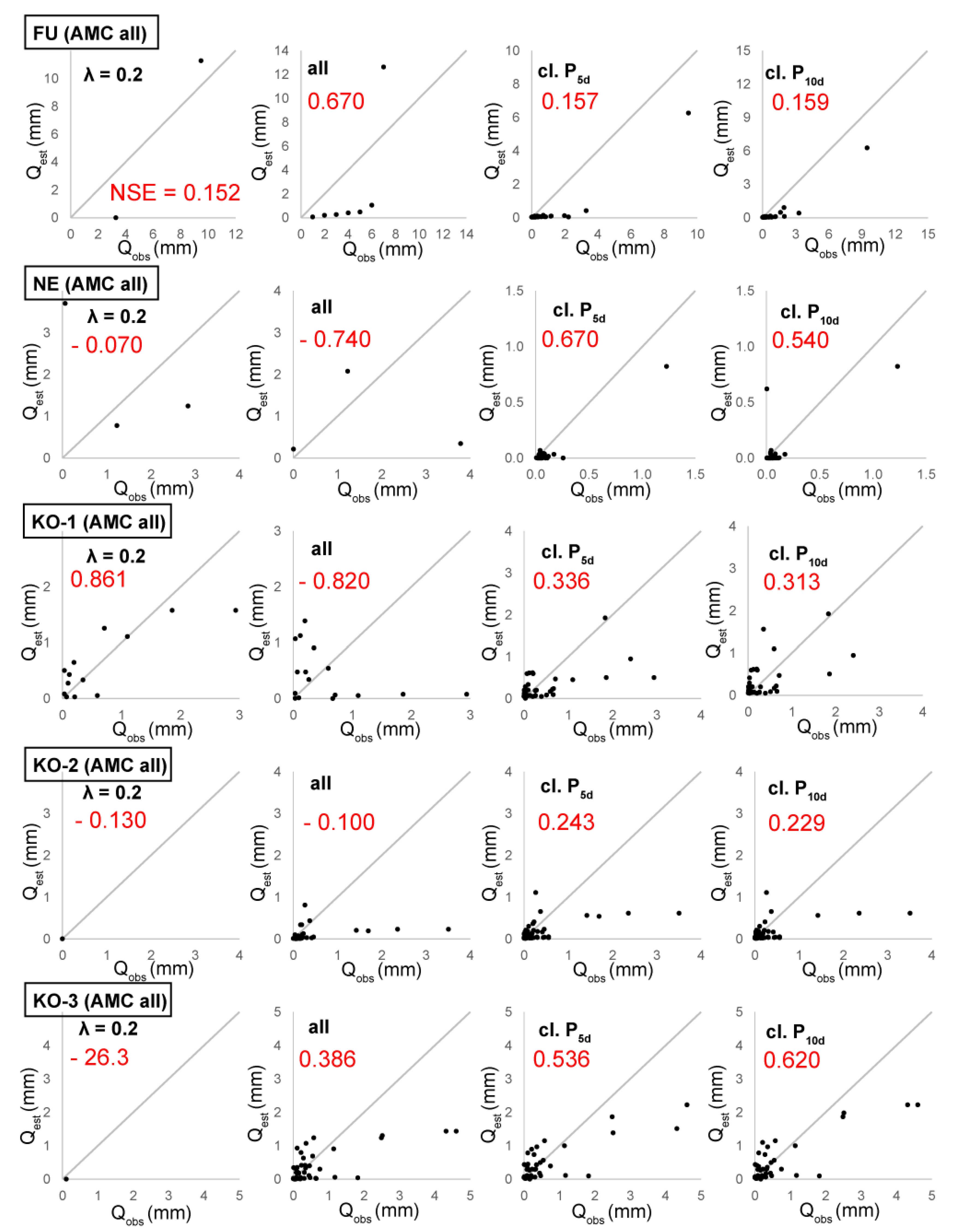
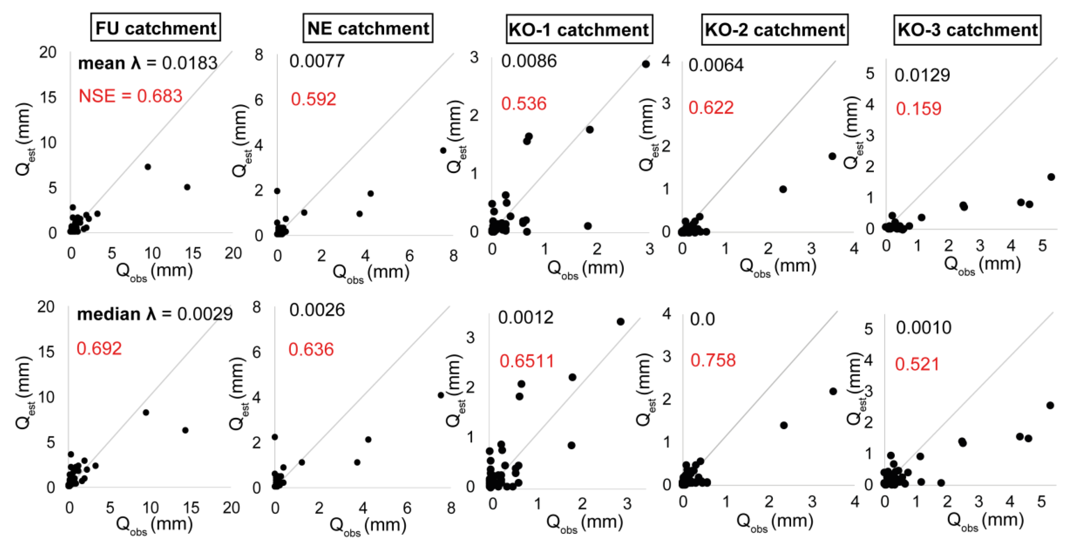
4.3.2. Model Fitting

The iterative model-fitting procedure was applied to training datasets in all studied catchments to identify pairs of S and λ values. As in previous analyses, computations were performed with and without the clustering (separation), according to the P5d and P10d thresholds. The S:λ pairs are provided in Table 9. Verification has shown that using the identified S:λ pairs leads to enhancement of estimated direct runoff, compared with those calculated through the original CN method. However, performance differs among catchments (Table 10, Figure 7). For simulations without the separation (all), NSE ranged from 0.146 to 0.585. NSE exceeded 0.500 in the FU and KO-3 catchments. For the P5d -based separation, NSE ranged from 0.362 to 0.671, and NSE was higher than 0.500 in the FU and KO-3 catchments. Finally, for the P10d-based separation, NSE ranged from 0.391 to 0.768, with NSE exceeding 0.500 in the NE and KO-3 catchments. In addition, here, the underestimating tendency is apparent for higher Q.

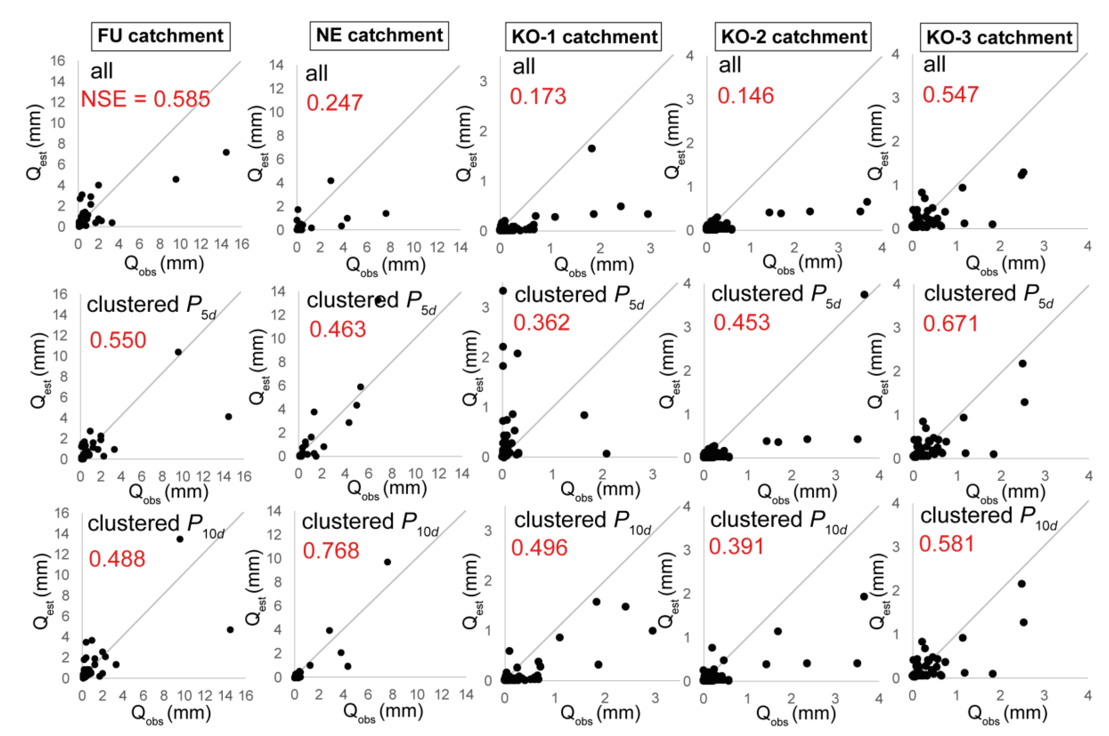
4.4. HEC-HMS Simulations

To simulate a surface-runoff process using HEC-HMS, calibration was conducted for two types of events: (1) Those with a slowly rising limb of the hydrograph, and (2) those with a rapid onset. In the calibrations, all parameters’ values (see Section 3.5 were optimised, and calibration coefficients were calculated for Ia, CN and Tc (Table 11). The remaining parameters’ values were taken as they had been calculated in the calibrations.
The HEC-HMS simulations indicate that changes in all surface-runoff-driving parameters led to improved results. For the event with the rising limb of the hydrograph rising rather slowly, significant improvement was achieved even for λ = 0.2 with modified parameters. In the original setting, the bias was −52.29% and NSE was −4.655 (see Figure 8a). In the simulation that employed the modified parameters, bias was only −3.17%, and NSE reached 0.918 (see Figure 8b). For the same event, a simulation using λ = 0.0142 with the original parameters’ values delivered solid output, with bias at −7.01% and NSE reaching 0.845 (see Figure 8c). Finally, computations using λ = 0.0142 and the recalculated parameters led to improvement in the simulation, as bias fell to −2.12%, and NSE increased to 0.912 (see Figure 8d).
The simulation of runoff response with a rapid onset was less accurate, as indicated in Figure 9. The computation employing λ = 0.2 with the original setting of the surface-runoff-driving parameters was insufficient (see Figure 9a). After recalculating the parameters, accuracy increased (NSE = 0.408), but absolute bias worsened. The modelled runoff depicted in Figure 9b shows an approximation to the real data in terms of temporal course. Analogous use of λ = 0.0142 delivered a more pronounced improvement in the modelled runoff, with bias falling from 55% to 3%, and NSE increasing from −0.194 to 0.695 (Figure 9c,d).
Bearing in mind that the number of simulations by the HEC-HMS performed in this study is low, one should avoid general interpretations. Nevertheless, the presented results outline how reducing Ia improves the model’s ability to deliver more accurate output, which is significantly more pronounced in the case of slow onset runoff, in which both the temporal course and runoff volume/level matched well with real runoff. In the case of rapid onset events, reducing λ from 0.2 to 0.0142 played a more significant role, as the best simulation was the one with λ = 0.0142 and recalculated parameters. However, the simulated hydrograph did not match well with the real results (Figure 9d). This indicates that the HEC-HMS simulation of such types of runoff events can deliver sufficiently accurate hydrographs in terms of runoff volume/level, although the culmination is inaccurate.

5. Discussion and Conclusions

Experience from various watersheds worldwide has highlighted the sensitivity of runoff to the initial abstraction coefficient [2,24,64]. In this study, initial abstraction coefficients λ were estimated for five experimental catchments in the Czech Republic, which well reflect the physiographic conditions (in terms of soil and geomorphology) in the Central European watersheds, using various approaches. From a methodological perspective, they can be divided into two types: (1) Approaches based on a classical determination of tabulated CN numbers [65], and (2) those based on a CN-independent analysis of rainfall-runoff data. The adjusted λ values were determined as discrete or function-dependent (interpolated). Contribution of this research lies in the comparison of different approaches of CN estimations applied in various watersheds.

5.1. Tabulated CN, Discrete λ

When using discrete λ values, these general conclusions based on our findings can be stated: λ differed both between studied catchments and between events, and the original value of 0.2 should be reduced in studied catchments, except the KO-1 catchment. Mean λ ranged from 0.0365 to 0.8330 and median λ from 0.0142 to 0.0913 for simulations that take the AMC classification into consideration. In simulations that omitted the AMC classification (AMC implicitly was set to II), λ values were slightly higher. Mean λ ranged from 0.0818 to 0.2846, and median λ ranged from 0.0479 to 0.2001; λ exceeded 0.2 in the KO-1 catchment, which is almost entirely covered by arable and land with specific infiltration conditions due to presence of tile drainage system [66], making this catchment very different from the others. The example of the KO-1 catchment well documents that correct CN determination must take into consideration artificial elements that are not reflected in the traditional methodology, yet their influence on runoff formation is significant.
Generally, the obtained results correspond with those of other authors, such as Baltas et al. [62], who reported mean λ = 0.034 and 0.014 for two watersheds. They attributed the various λ results to differences in the presence of impervious formations and urban development. Similarly, Shi et al. [11] reported λ ranging from 0.010 to 0.152, with a median of 0.048 due to landscape and geological characteristics. Lal et al. [13] conducted research in different agricultural plots in India and found that the mean and median for λ were 0.0 and 0.034. Krajewski et al. [24] compared λ values in 2 catchments in Poland and found average λ = 0.026 and 0.047.

5.2. Tabulated CN, Interpolated λ

Some approaches exist for expressing λ as being functionally (linearly) dependent on precipitation. For example, Kohnová et al. [69] conducted research in Slovakian watersheds and expressed λ as a linear function of precipitation for each AMC class. Moreover, they also discussed the low number of II and III AMC classes. Therefore, they stated that no apparent relationship existed between CN and AMC, and that other parameters’ roles should be emphasised. Application of linear λ:P relationships in this study increased runoff estimates’ overall accuracy compared with the original CN method. Like the discrete λ, NSE only exceeded 0.500 in one catchment—the KO-3 catchment with AMC classified, and in the KO-1 catchment without AMC classification. Generally speaking, the ability of λ:P linear regressions used for runoff simulations appears to be rather weak, which can be attributed to unknown interplay among other characteristics taking part in the direct-runoff formation, or to inappropriate tabulated CNs. Moreover, a question arises of the need of training datasets large enough, from which representative regression equations can be derived. Despite the sufficient amount of training events in this study (from 44 to 80), there is a problem of lack of extreme/severe events, in which the runoff formation may be very specific.
Recently, a different interpolating approach has been successfully tested by Krajewski et al. [24], approximating the λ–P relationship with an asymptotic formula. They found greater variability in λ values for smaller P. After exceeding a certain threshold P, λ approaches a constant value. The threshold depends on a catchment’s characteristics, namely land cover that strongly influences the direct runoff formation or initial abstraction, separately. Based on the promising results of this asymptotic approach, the method definitely deserves to be tested in wider range of geographical conditions.

5.3. Summary of Tabulated CN-Based Approaches

Modification of λ in calculations using tabulated CNs led to a partial increase in the accuracy of direct-runoff estimates, but because NSE often did not exceed 0.500, overall performance seems to be rather unambiguous. More specifically, it is apparent that the estimates for smaller Q were more accurate than for those with higher Q. This issue might be resolved based on sophisticated statistical analyses that were beyond the scope of this study.
Both discussed approaches’ inaccuracy indicates that the tabulated CNs [65] used in the Czech Republic often are not representative, thereby requiring a systematic revision that should be based on analyses of a large amount of data from various watersheds in the Central European region, ensuring the CN method’s robustness. Moreover, just as it seems inappropriate to use the universal initial abstraction coefficient λ value for different river basins, it certainly would be more appropriate to use the CN method, taking into account the spatio-temporal variability of runoff conditions resulting from seasonal variability in CN and λ regarding vegetation variability and distribution of soil and land use [24,30,31,32]. Extant studies have dealt with this issue, such as one conducted by Hawkins et al. [2], who concluded that lower CNs prevailed during the summer (growing season) and that higher CNs better represented runoff conditions during the dormant season. In a recent study by Muche et al. [79], CNs were derived using the Normalised Difference Vegetation Index (NDVI) to reflect seasonal land-use changes in the hydrologic circle. They concluded that the CN-NDVI method is a promising alternative to the traditional CN method. In the present study, the CORINE Land Cover dataset was refined using aerial images together with annual data on crop distribution on arable land, where available. It is reasonable to assume that by using appropriate satellite data, the estimated CNs would better represent the spatial distribution of land-cover features, vegetation and also soil moisture. However, this went beyond the scope of this research. Moreover, it should be noted that the Central European region currently is facing the bark beetle calamity and a drought affecting large areas of forest stands (mostly with spruces). This should be taken into account during determination of CNs, although the calamity did not affect the studied catchments. In this regard, it should also be added that the issue of a single CN value characterising the entire catchment’s conditions has been addressed by Soulis and Valiantzas [30,31] who implemented a two-CN system approach in heterogeneous watersheds and improved the CN method’s performance. Even in a watershed affected by massive changes caused by a forest fire, this approach performed well [32]. Thus, efficient methods exist, offering opportunity to be used in the process of new CN determination (revision), not only in the Czech Republic.

5.4. Tabulated CN-Independent Approaches

To estimate optimal λ and S values, two methods without using tabulated CNs were applied: (1) Event analysis based on analysing individual events’ rainfall-runoff parameters, and (2) model fitting—an iterative numerical procedure searching for a pair of λ and S values that best describe a particular catchment’s runoff conditions.
The event analysis yielded the best results from all the methods compared in this research. In all studied catchments, the application of S-P10d regressions combined with mean (ranging from 0.0064 to 0.0129) and median λ (ranging from 0.0 to 0.0029) led to significant increases in estimated direct-runoff accuracy. With one exception (KO-3 catchment with mean λ applied), NSE always exceeded 0.500.
The model-fitting procedure also produced more accurate outputs compared with the original CN method, both with and without using the clustering (separation) according to the P5d and P10d thresholds. NSE exceeded 0.500 in only two out of the five studied catchments. This probably is caused by the fact that using a single pair of λ and S values that universally represent runoff conditions in a catchment in a wide range of rainfall and land-cover arrangements is questionable [24,30]. Another problem resides in the lack of events with high Q, of which the behaviour is strongly variable, and thus significantly influences the calculation of the λ:S pairs.

5.5. HEC-HMS Simulations Using Adjusted λ and CN

Application of adjusted λ values in HEC-HMS shows that using lower λ leads to improvements in simulated runoff accuracy, but a difference exists between hydrographs with slow and rapid onsets: Both yielded sufficiently accurate results in terms of runoff volume. However, within the hydrograph with rapid onset, the model was unable to match the culmination discharge. This might indicate a lower performance in the HEC-HMS SCS-CN-based simulations to model events with fast runoff response, especially flash floods, in terms of peak discharge, which often is the parameter of the main interest. At the same time, it should be emphasised that general interpretations would require an analysis on a representative dataset of rainfall-runoff events. In this present study, the aim was to examine preliminarily the applicability of modified λ values within HEC-HMS software.

5.6. Summary

The present study shows that the original CN methodology without adjustments to local conditions is hardly applicable in the geographical conditions of the experimental watersheds. Both CN and λ values should be based on site-specific characteristics, i.e., on rainfall-runoff data observations, hinting that they should be viewed as flexible regional parameters, rather than fixed values. In the studied catchments’ specific natural conditions, the λ appears mostly to be considerably lower than the original value of 0.2. As the CN method frequently is used in long-term and event-based runoff simulations, erosion modelling and wide range of other applications, appropriate modifications of the method, such as those presented in this study, can contribute significantly to improvements in their outputs. It is the authors’ intention to extent the present research and take up the unresolved problems, such as the systematic underestimation of direct runoff for events with higher runoff observed. Moreover, testing the possibilities of revisiting CN determination, mainly with regard to watersheds’ heterogenity, as well as investigation of the regionalised concepts in the natural and agricultural conditions of the Czech Republic and neighbouring countries appears to be a challenging issue deserving our attention. This study’s outcomes may serve as a preliminary basis for subsequent activities addressing the aforementioned tasks.

Supplementary Materials

The following are available online at https://www.mdpi.com/2073-4441/12/7/1964/s1, Figure S1a: Comparison of observed direct runoff heights (mm) with those simulated in the experimental catchments using discrete mean and median λ values with AMC classified (AMC all), Figure S1b: Comparison of observed direct runoff heights (mm) with those simulated in the experimental catchments using discrete mean and median λ values with AMC implicitly set as normal (AMC = II), Figure S2: Comparison of observed direct runoff heights (mm) with those simulated in the experimental catchments using regressions of λ according to P for events with AMC classified (AMC all) and implicitly set as normal (AMC = II).

Author Contributions

Conceptualisation, M.C.; methodology, M.C., M.Š.M.; validation, M.C.; formal analysis, M.C., M.Š.M.; P.F.; investigation, M.C.; writing-original draft preparation, M.C., M.Š.M.; writing-review and editing, M.C., M.Š.M., P.F., P.K.; visualisation, M.C. All authors have read and agreed to the published version of the manuscript.

Funding

This research was funded by the DEPARTMENT OF GEOGRAPHY, FACULTY OF SCIENCE, MASARYK UNIVERSITY, grant number MUNI/A/1251/2019, T. G. MASARYK WATER RESEARCH INSTITUTE, internal grant number 1628 and 3600.52.27/2020 and by the MINISTRY OF AGRICULTURE OF THE CZECH REPUBLIC, grant number MZE RO0218.

Acknowledgments

The authors would like to thank the Povodí Odry State Enterprise and Research Institute for Soil and Water Conservation for providing the input rainfall and runoff data. The authors also would like to thank the anonymous reviewers for their constructive comments and recommendations, which helped to improve the paper.

Conflicts of Interest

The authors declare no conflict of interest.

References

  1. Bonta, J.V. Determination of Watershed Curve Number Using Derived Distributions. J. Irrig. Drain. Eng. 1997, 123, 28–36. [Google Scholar] [CrossRef]
  2. Woodward, D.E.; Hawkins, R.H.; Jiang, R.; Hjelmfelt, A.T., Jr.; Van Mullem, J.A.; Quan, Q.D. Runoff curve number method: Examination of the initial abstraction ration. In Proceedings of the World Water and Environmental Resources Congress, Philadelphia, PA, USA, 23–26 June 2003; Bizier, P., De Barry, P., Eds.; pp. 691–700. [Google Scholar]
  3. USDA. Soil Conservation Service, National Engineering Handbook Supplement: Supplement A, Hydrology; USDA: Washington, DC, USA, 1956. [Google Scholar]
  4. USDA. Soil Conservation Service, National Engineering Handbook. Section 4: Hydrology; USDA: Washington, DC, USA, 1972; p. 762. [Google Scholar]
  5. USDA. Urban Hydrology for Small Watersheds, 2nd ed.; Technical Release 55; USDA: Washington, DC, USA, 1986; p. 164. [Google Scholar]
  6. USDA. National Engineering Handbook, Part 630, Hydrology; USDA: Washington, DC, USA, 2004. [Google Scholar]
  7. Hawkins, R.H.; Ward, T.J.; Woodwards, E.; Van Mullem, J.A. Continuing evolutioon of rainfall-runoff and the curve number precedent. In Proceedings of the 2nd Federal Inegracy Conference, Las Vegas, NV, USA, 27 June–1 July 2010. [Google Scholar]
  8. Mishra, S.K.; Vijay, P.; Singh, P.K. Revisiting the Soil Conservation Service curve number method. In Proceedings of the International Conference on Water, Environment, Energy and Society, Bhopal, India, 15–18 March 2016; Singh, V.P., Yadav, S., Yadava, R.N., Eds.; Springer: Singapore, 2018; pp. 667–693. [Google Scholar]
  9. Ponce, V.M.; Hawkins, R.H. Runoff curve number: Has it reached maturity? J. Hydrol. Eng. 1996, 1, 11–19. [Google Scholar] [CrossRef]
  10. Satheeshkumar, S.; Venkateswaran, S.; Kannan, R. Rainfall-runoff estimation using SCS-CN and GIS approach in the Pappiredipatti watershed of the Vaniyar sub basin, South India. Mod. Earth Sys. Environ. 2017, 3. [Google Scholar] [CrossRef]
  11. Shi, Z.H.; Chen, L.D.; Fang, N.F.; Qin, D.F.; Cai, C.F. Research on the SCS-CN initial abstraction ratio using rainfall-runoff event analywsis in the Three Gorges Area, China. Catena 2009, 77, 1–7. [Google Scholar] [CrossRef]
  12. Jacobd, J.H.; Srinivasan, R. Effects of curve number modification on runoff estimation using WSR-88D raifall data in Texas watersheds. J. Soil Water Conserv. 2005, 60, 274–279. [Google Scholar]
  13. Lal, M.; Mishra, S.K.; Pandey, A. Physical verification of the effect of land features and antecedent moisture on runoff curve number. Catena 2015, 133, 318–327. [Google Scholar] [CrossRef]
  14. Springer, E.P.; McGurk, B.J.; Hawkins, R.H.; Coltharp, G.B. Curve numbers from watershed data. In Proceeding of the Symposium on Watershed Management, Boise, ID, USA, 21–23 July 1980; ASCE: New York, NY, USA, 1980; pp. 938–950. [Google Scholar]
  15. Mishra, S.K.; Chaudhary, A.; Shrestha, R.K.; Pandey, A.; Lal, M. Experimental Verification of the Effect and Land Use on SCS Runoff Curve Number. Water Resour. Manag. 2014, 28, 3407–3416. [Google Scholar]
  16. Hawkins, R.H.; Ward, T.J.; Woodwards, E.; Van Mullem, J.A. Curve Number Hydrology: State of the Practice; ASCE: Reston, VA, USA, 2009; p. 106. [Google Scholar]
  17. Jha, M.K.; Chovdary, V.M.; Kulkarni, Y.; Mal, B.C. Rainwater harvesting planning using geospatial techniques and multicriteria decision analysis. Res. Conserv. Recycl. 2014, 83, 96–111. [Google Scholar] [CrossRef]
  18. Sharpley, A.N.; Williams, J.R. EPIC Erosion/Productivity Impact Calculator: 1. Model Documentation. In USA Department of Agriculture Technical Bulletin No. 1768; Government Printing Office: Washington, DC, USA, 1990. [Google Scholar]
  19. Ajmal, M.; Moon, G.; Ahn, J.; Kim, T. Investigation of SCS-CN and its inspired modified models for runoff estimation in South Korean watersheds. J. Hydro-Environ. Res. 2015, 9, 592–603. [Google Scholar] [CrossRef]
  20. Ajmal, M.; Khan, T.A.; Kim, T.W. A CN-Based Ensembled Hydrological Model for Enhanced Watershed Runoff Prediction. Water 2016, 8, 20. [Google Scholar] [CrossRef] [Green Version]
  21. Mishra, S.K.; Singh, V.P. SCS-CN-based hydrologic simulation package. In Mathematical Models in Small Watershed Hydrology; Singh, V.P., Frevert, D.K., Eds.; Water Resources Publications: Littleton, CO, USA, 2002; pp. 391–464. [Google Scholar]
  22. Hjelmfelt, A.T. Ivestigation of curve number procedure. J. Hydraul. Eng. 1991, 117, 725–737. [Google Scholar] [CrossRef]
  23. Randusová, B.; Marková, R.; Kohnová, S.; Hlavčová, K. Comparison of cn estimation approaches. Int. J. Eng. Sci. 2015, 1, 34–40. [Google Scholar]
  24. Krajewski, A.; Sikorska-Senoner, A.E.; Hejduk, A.; Hejduk, L. Variability of the Initial Abstraction Ratio in an Urban and an Agroforested Catchment. Water 2020, 12, 471. [Google Scholar] [CrossRef] [Green Version]
  25. Hjelmfelt, A.T. Empirical investigation of curve number technique. J. Hydraul. Div. ASCE 1980, 106, 1471–1476. [Google Scholar]
  26. Hawkins, R.H. Discussion of ‘Empirical Ivestigation of Curve Number Technique’, by A. T. Hjelmfelt. J. Hydraul. Div. ASCE 1981, 107, 953–954. [Google Scholar]
  27. Hawkins, R.H.; Hjelmfelt, A.T.; Zevenbergen, A.W. Runoff probability, relative storm depth, and runoff curve numbers. J. Irrig. Drain. Eng. 1985, 111, 330–340. [Google Scholar] [CrossRef]
  28. Hawkins, R.H. 1993 Asymptotic determination of runoff curve numbers from data. J. Irrig. Dran. Div. ASCE 1993, 119, 334–345. [Google Scholar] [CrossRef]
  29. Ajmal, M.; Kim, T. Quantifying excess stormwater using SCS-CN-based rainfall runoff models and different curve number determination methods. J. Irrig. Drain. Eng. 2015, 141. [Google Scholar] [CrossRef]
  30. Soulis, K.X.; Valiantzas, J.D. SCS-CN parameter determination using rainfall-runoff data in heterogenous watersheds—The two-CN system approach. Hydrol. Earth Syst. Sci. 2012, 16, 1001–1015. [Google Scholar] [CrossRef] [Green Version]
  31. Soulis, K.X.; Valiantzas, J.D. Identification of the SCS-CN Parameter Spatial Distribution Using Rainfall-Runoff Data in Heterogenous Watersheds. Water. Resour. Manage. 2013, 27, 1737–1749. [Google Scholar] [CrossRef]
  32. Soulis, K.X. Estimation of SCS Curve Number variation following forest fires. Hydrol. Sci. J. 2018, 63, 1332–1346. [Google Scholar] [CrossRef]
  33. Rees, H.W.; Chow, T.L.; Gregorch, E.G. Soil and crop responses to long-term potato production at a benchmark site in northwestern New Brunswick. Can. J. Soil Sci. 1988, 88, 409–422. [Google Scholar] [CrossRef]
  34. Wang, X.; Liu, T.; Yang, W. Development of a robust runoff-prediction model by fusing the Rational Equation and modified SCS-CN method. Hydrol. Sci. J. 2012, 57, 1118–1140. [Google Scholar] [CrossRef] [Green Version]
  35. Mishra, S.K.; Pandey, R.P.; Jain, M.K.; Singh, V.P. A rain duration and modified AMC-dependent SCS-CN procedure for long duration rainfall-runoff events. Water Resour. Manag. 2008, 22, 861–876. [Google Scholar] [CrossRef]
  36. Neitsch, S.L.; Arnold, J.G.; Kiniry, J.R.; Williams, J.R.; King, K.W. Soil and Water Assessment Tool (SWAT): Theoretical Documentation, Version 2000; Texas Water Resources Institute: College Station, TX, USA, 2002; p. 506. [Google Scholar]
  37. Sobhani, G. A Review of Selected Small Watershed Design Methods for Possible Adoption to Iranian Conditions. Master’s Thesis, Utah State University, Logan, UT, USA, 1975. [Google Scholar]
  38. Mishra, S.K.; Singh, V.P.; Sansalone, J.J.; Aravamuthan, V. A modified SCS-CN method: Characterization and testing. Water Resour. Manag. 2003, 17, 37–68. [Google Scholar] [CrossRef]
  39. Ponce, V.M. Engineering Hydrology, Principles and Practices; Prentice Hall: Englewood Cliffs, NJ, USA, 1989; p. 640. [Google Scholar]
  40. Williams, J.R.; LaSeur, W.V. Water yield model using SCS curve numbers. J. Hydraul. Div. 1976, 102, 1241–1253. [Google Scholar]
  41. Hawkins, R.H. Runoff curve numbers with varying site moisture. J. Irrig. Drain. Div. 1978, 104, 389–398. [Google Scholar]
  42. Mishra, S.K.; Jain, M.K.; Singh, V.P. Evaluation of the SCS-CN-based model incorporating antecedent moisture. Water Resour. Manag. 2004, 18, 567–589. [Google Scholar] [CrossRef]
  43. Mishra, S.K.; Singh, V.P. Long-term hydrological simulation based on the Soil Conservation Service curve number. Hydrol. Process. 2004, 18, 1291–1313. [Google Scholar] [CrossRef]
  44. Michel, C.; Andréassian, V.; Perrin, C. Soil Conservation Service Curve Number method: How to mend a wrong soil moisture accounting procedure? Water Resour. Res. 2005, 41. [Google Scholar] [CrossRef]
  45. Jain, M.K.; Durbude, D.G.; Mishra, S.K. Improved CN-based long-term hydrologic simulation model. J. Hydrol. Eng. 2012, 17, 1204–1220. [Google Scholar] [CrossRef]
  46. Sahu, R.K.; Mishra, S.K.; Eldho, T.I.; Jain, M.K. An advanced soil moisture accounting, procedure for SCS curve number method. Hydrol. Process. 2007, 21, 2872–2881. [Google Scholar] [CrossRef]
  47. Singh, P.K.; Mishra, S.K.; Berndtsson, R.; Jain, M.K.; Pandey, R.P. Development of modified SMA based MSCS-CN model for Runoff Estimation Water. Resour. Manag. 2015, 29, 4111–4127. [Google Scholar]
  48. Verma, S.; Mishra, S.K.; Singh, A.; Singh, P.K.; Verma, R.K. An enhanced SMA based SCS-CN inspired model for watershed runoff prediction. Environ. Earth Sci. 2017, 76. [Google Scholar] [CrossRef]
  49. Verma, S.; Singh, P.K.; Mishra, S.K.; Jain, S.K.; Berndtsson, R.; Singh, A.; Verma, R.K. Simplified SMA-inspired 1-parameter SCS-CN model for runoff estimation. Arab. J. Geosci. 2018, 11. [Google Scholar] [CrossRef]
  50. Desmukh, D.S.; Chaube, U.C.; Hailu, A.E.; Gudeta, D.A.; Kassa, M.T. Estimation and comparison of curve numbers based on dynamic land use cover change, observed rainfall-runoff data and land slope. J. Hydrol. 2013, 492, 89–101. [Google Scholar] [CrossRef]
  51. Huang, M.; Gallichand, J.; Wang, Z.; Goulet, M. A modification to the Soil Conservation Service curve number method for steep slopes in the Loess Plateau of China. Hydrol. Process. 2006, 20, 579–589. [Google Scholar] [CrossRef]
  52. Plummer, A.; Woodward, D.E. The origin and Derivation of Ia/S in the Runoff Curve Number System. In Proceedings of the International Water Resources Engineering Conference, Memphis, TN, USA, 3–7 August 1998; Abt, S.R., Yoing-Pezeshk, J., Watson, C.C., Eds.; ASCE: Reston, VA, USA, 1998; pp. 1260–1265. [Google Scholar]
  53. Fu, S.; Zhang, G.; Wang, N.; Luo, L. Initial abstraction ratio in the SCS-CN method in the Loess Plateau of China. Trans. ASABE 2011, 54, 163–169. [Google Scholar] [CrossRef]
  54. Fan, F.; Deng, Y.; Hu, X.; Weng, Q. Estimating Composite Curve Number Using an Improved SCS-CN Method with Remotely Sensed Variables in Guangzhou, China. Remote Sens. 2013, 5, 1425–1438. [Google Scholar] [CrossRef] [Green Version]
  55. Reistetter, J.A.; Russell, M. High-resolution land cover datasets, composite curve numbers, and storm water retention in the Tampa Bay, FL region. Appl. Geogr. 2011, 31, 740–747. [Google Scholar] [CrossRef]
  56. Mockus, V. Design Hydrographs. In National Engineering Handbook; Section 4, Hydrology; McKeever, V., Owen, W., Rallison, R., Eds.; Soil Conservation Service: Washington, DC, USA, 1972. [Google Scholar]
  57. Cazier, D.J.; Hawkins, R.H. Regional application of the curve number method. Water Today and Tomorrow. In Proceedings of the ASCE, Irrigation and Drainage Division Special Conference, Flagstaff, AZ, USA, 24–26 July 1984; Replogle, J.A., Ed.; ASCE: New York, USA, 1984. [Google Scholar]
  58. Mishra, S.K.; Singh, V.P. Another look at SCS-CN method. J. Hydrol. Eng. 1999, 4, 257–264. [Google Scholar] [CrossRef]
  59. Hawkins, R.H.; Khojeini, A.V. Initial Abstraction and Loss in the Curve Number Method Hydrol; Arizona-Nevada Academy of Science. Water Resour. Ariz. Southwest 2000, 30, 29–35. [Google Scholar]
  60. Jiang, R. Investigation of Runoff Curve Number Initial Abstraction Ratio. Master’s Thesis, The University of Arizona, Tucson, AZ, USA, 2001. [Google Scholar]
  61. Lim, K.J.; Engel, B.A.; Muthukrishnan, S.; Harbor, J. Effects of initial abstraction and urbanization of estimated runoff using CN technology. J. Am. Water Resour. Assoc. 2006, 42, 629–643. [Google Scholar] [CrossRef]
  62. Baltas, E.A.; Dervos, N.A.; Mimikou, M.A. Technical Note: Determination of the SCS initial abstraction ratio in an experimental watershed in Greece. Hydrol. Earth Sys. Sci. 2007, 11, 1825–1829. [Google Scholar] [CrossRef] [Green Version]
  63. Xiao, B.; Wang, Q.H.; Fan, J.; Han, F.P.; Dai, Q.H. Application of the SCS-CN model to runoff estimation on a small watershed with high spatial heterogeneity. Pedosphere 2011, 21, 738–749. [Google Scholar] [CrossRef]
  64. Yuan, Y.; Nie, W.; McCutcheon, S.C.; Taguas, E. Initial abstraction and curve numbers for semiarid watersheds in Southeastern Arizona. Hydrol. Process. 2014, 28, 774–783. [Google Scholar] [CrossRef]
  65. Janeček, M.; Dostál, T.; Dufková, J.K.; Dumbrovský, M.; Hůla, J.; Kadlec, V.; Konečná, J.; Kovář, P.; Krása, J.; Kubátová, E.; et al. Ochrana zemědělské půdy před erozí; Czech University of Life Sciences: Prague, Czech Republic, 2012; p. 113. [Google Scholar]
  66. Caletka, M.; Honek, D. Improving direct runoff estimations through modifying SCS-CN initial abstraction ratio in a catchment prone to flash floods. In Proceedings of the International Multidisciplinary Scientific GeoConference Surveying Geology and Mining Ecology Management, lbena, Bulgaria, 28 June–7 July 2019; pp. 281–288. [Google Scholar]
  67. Caletka, M.; Michalková, M.Š. Determination of SCS-CN initial Abstraction ratio in a chatchment prone to flash floods. Pollack Per. 2020, 15, 112–123. [Google Scholar]
  68. Karabová, B. Testovanie možnosti regionalizácie vybraných parametrov metódy SCS-CN—Oblast nížin Slovenska. Acta Hydrol. Slovaca 2013, 15, 194–203. [Google Scholar]
  69. Kohnová, S.; Karabová, B.; Hlavčová, K. On the possibilities of watershed parametrization of extreme flow estimation on ungauged basins. In Proceedings of the Congress in Flood Risk and Precipitation in Catchments and Cities, Prague, Czech Republic, 22 June–2 July 2015; Chen, Y., Estupina, V.B., Schumann, A., Aksoy, H., Bloschl, G., Kooy, M., Rogger, M., Toth, E., Eds.; Copernicus GmbH: Göttingen, Germany, 2015; pp. 171–175. [Google Scholar]
  70. Kohnová, S.; Rutkowska, A.; Banasik, K.; Hlavčová, K. The L-moment based regional approach to curve numbers for Slovak and Polish Carpathian catchments. J. Hydrol. Hydromech. 2020, 68, 1–10. [Google Scholar] [CrossRef]
  71. Daňhelka, J.; Kubát, J. Vyhodnocení Povodní v Červnu a Červenci 2009 (Assessment of Floods in June and July 2009 in the Czech Republic); Ministry of Environment, CHMI: Prague, Czech Republic, 2009; p. 165. [Google Scholar]
  72. Šunka, Z. Vyhodnocení Povodní v Květnu a Červnu 2010 (Assessment of Floods in May and June 2010); Ministry of Environment, TGM WRI: Prague, Czech Republic, 2010; p. 172. [Google Scholar]
  73. Honek, D.; Michalková, M.Š.; Smetanová, A.; Sočuvka, V.; Velísková, Y.; Karásek, P.; Konečná, J.; Némethová, Z.; Danáčová, M. Estimating sedimentation rates in small reservoirs—Suitable approaches for local municipalities in central Europe. J. Environ. Manag. 2020, 261. [Google Scholar] [CrossRef] [PubMed]
  74. Goovaerts, P. Geostatistical approaches for incorporating elevation into the spatial interpolation of rainfall. J. Hydrol. 2000, 228, 113–129. [Google Scholar] [CrossRef]
  75. Yang, K.; Cao, S.; Liu, X. Flow resistance and its precipitation methods in compound channels. Acta Mech. Sin. 2007, 23, 23–31. [Google Scholar] [CrossRef]
  76. Pham, D.T.; Dimov, S.S.; Nguyen, C.D. Selection of K in K-means clustering. J. Mech. Eng. Sci. 2005, 219, 103–119. [Google Scholar] [CrossRef] [Green Version]
  77. Dingman, S.L. Physical Hydrology, 2nd ed.; Macmillan Press Limited: New York, NY, USA, 2002; p. 646. [Google Scholar]
  78. Konečná, J.; Karásek, P.; Beitlerová, H.; Fučík, P.; Kapička, J.; Podhrázská, J.; Kvítek, T. Using WaTEM/SEDEM and HEC-HMS episodic models for the simulation of episodic hydrological and erosion events in a small agricultural catchment. Soil Water Res. 2019, 15, 18–29. [Google Scholar] [CrossRef]
  79. Muche, M.E.; Hutchinson, S.L.; Hutchinson, J.M.S.; Johnston, J.M. Phenology-adjusted dynamic curve number for improved hydrologic modelling. J. Environ. Manag. 2019, 235, 403–413. [Google Scholar] [CrossRef]
Figure 1. Overview map of the experimental catchments.
Water 12 01964 g001
Figure 2. Surface, land cover classification and curve number (CN) determination.
Water 12 01964 g002
Figure 3. Principal component analysis PCA conducted for rainfall-runoff events in the experimental catchments.
Water 12 01964 g003
Figure 4. Initial abstraction coefficient λ expressed as linear function of precipitation height P for the experimental catchments and for AMC classified (AMC all) and normal only (AMC = II).
Water 12 01964 g004
Figure 5. Comparison of observed direct runoff heights (mm) with those simulated in the experimental catchments using regressions of λ according to P for events with AMC classified (AMC all). Comparison of direct runoff estimates with AMC not classified (AMC = II) is provided in Figure S2.
Water 12 01964 g005
Figure 6. Comparison of observed direct runoff heights with those simulated in the experimental catchments using regressions of S according to P10d (event analysis) with application of mean and median λ.
Water 12 01964 g006
Figure 7. Comparison of observed direct runoff heights with those simulated using pairs of S and λ identified by means of model fitting procedure. The validation was carried out both with (all) and without delimitation of clusters according to P5d (clustered P5d) and P10d (clustered P10d).
Water 12 01964 g007
Figure 8. Verification of surface runoff simulations of a runoff event with a slower onset in the NE catchment using the HEC-HMS software. The simulations were computed using original Ia, CN and Tc values corresponding to λ = 0.2 (a), modified Ia, CN and Tc values corresponding to λ = 0.2 (b), original Ia, CN and Tc values corresponding to λ = 0.0142 (c) and finally modified Ia, CN and Tc values corresponding to λ = 0.0142 (d). The model’s performance is expressed by the bias of runoff heights and Nash–Sutcliffe model efficiency (NSE) coefficient.
Water 12 01964 g008
Figure 9. Verification of surface runoff simulations of a runoff event with a rapid onset in the NE catchment using the HEC-HMS software. The simulations were computed using original Ia, CN and Tc values corresponding to λ = 0.2 (a), modified Ia, CN and Tc values corresponding to λ = 0.2 (b), original Ia, CN and Tc values corresponding to λ = 0.0142 (c) and modified Ia, CN and Tc values corresponding to λ = 0.0142 (d). The model’s performance is expressed by the bias of runoff heights and NSE coefficient.
Water 12 01964 g009
Table 1. Basic characteristics of the experimental catchments and percentage of land use categories (AL—arable land; BG—bare ground; FO—forest; GR—grassland and meadows; GA—gardens and orchards; PA—paved and built-up areas; SH—shrubbery; WA—water bodies).
Sub-CatchmentArea (km2)Elevation (m)Mean Slope (°)Mean P (mm)Mean Q (m3/s)Mean T (°C)
Min.Max.AnnualIV-IXAnnualIV-IX
FU57.82825636.16754500.3508.013.5
NE2.85596504.26504000.0157.014.0
KO-10.164905323.26754250.0076.512.5
KO-20.785486234.36754250.0036.512.5
KO-37.14786235.26754250.0266.512.5
Sub-CatchmentPercentage of Land Use Category (%)
ALBGFOGRGAGAPASHWA
FU43.50.024.723.75.25.21.41.30.2
NE50.90.231.85.25.45.43.13.40.0
KO-197.30.00.10.01.31.30.70.60.0
KO-252.20.044.41.10.60.60.11.50.0
KO-341.80.037.98.06.16.10.95.20.1
Table 2. Overview of rainfall and level/runoff measurements in the study catchments; Number of events chosen for training and validating datasets.
Sub-CatchmentPeriodNumber of Rain Gauges (Interval)Level/Runoff Measurement (Interval)Number of Events Chosen (Train./Valid.)
FU2008–201617 (10 min)Level gauge (1 h)44/45
NE2008–20171 (10 min)Thomson weir (10 min)57/81
KO-12005–20181 (10 min)Thomson weir (10 min)56/52
KO-22005–20181 (10 min)Thomson weir (10 min)73/74
KO-32005–20181 (10 min)Cippoletti weir (10 min)80/60
Table 3. Overview of methods employed in surface runoff simulations using HEC-HMS.
MethodParameter
LossSCS Curve NumberInitial abstraction (mm)
Curve Number (-)
Impervious (%)
TransformClark Unit HydrographTime of concentration (hr)
Storage coefficient (hr)
BaseflowInitial discharge (m3/s)
Recession constant (-)
Ratio (-)
Table 4. Quantitative outputs of the principal component analysis (PCA) for each study catchment: Percentage of variability explained by PC1 and PC2 along with the loading values for each input parameter.
Sub-CatchmentFUNEKO-1KO-2KO-3
Explained VariabilityPC 1
71.2%
PC 2
13.8%
PC 1
48.3%
PC 2
33.3%
PC 1
49.1%
PC 2
39.5%
PC 1
54.9%
PC 2
30.8%
PC 1
51.2%
PC 2
32.4%
P−0.070.81−0.040.460.320.11−0.080.44−0.180.41
duration−0.020.47−0.01−0.02−0.020.000.020.000.02−0.01
P5d0.450.320.51−0.04−0.250.560.590.090.500.20
P10d0.89−0.090.85−0.09−0.340.710.770.240.770.34
max. int.−0.070.070.130.880.850.40−0.240.86−0.350.81
Q0.040.110.010.030.000.000.000.01−0.010.04
Ia−0.010.010.000.020.000.01−0.010.02−0.050.11
Table 5. Mean and median values of events’ parameters (duration (h), P (mm), P5d (mm), P10d (mm), max. int. (mm/h), Q (mm), Ia (mm)) in the delimited clusters for the experimental catchments.
FUNEKO-1KO-2KO-3
MeanMed. MeanMed. MeanMed. MeanMed. MeanMed.
durationall (n = 45)12.0210.00all (n = 81)3.622.67all (n = 56)4.002.92all (n = 73)3.502.67all (n = 80)3.472.75
P17.414.010.86.917.111.513.910.014.310.0
P5d25.720.116.611.318.411.914.79.214.48.7
P10d42.935.330.122.228.821.225.018.827.219.9
max. int.10.688.3014.407.8023.1213.8019.1112.6019.8812.30
Q1.8300.3370.4480.0760.3160.0810.2930.0690.5670.101
Ia1.50.81.71.42.41.80.80.02.41.1
durationcl. 1 (n = 31)12.039.00cl. 1 (n = 58)3.812.92cl. 1 (n = 48)3.692.92cl. 1 (n = 68)3.412.80cl. 1 (n = 52)3.372.67
P18.514.111.37.117.811.414.010.016.310.8
P5d17.113.38.36.711.810.211.28.57.05.4
P10d26.226.418.117.022.418.821.817.213.713.7
max. int.11.438.9013.707.8024.4014.4019.4312.9022.8012.60
Q1.1520.3010.3190.0650.3080.0560.2460.0520.6330.090
Ia1.60.81.71.52.41.60.80.02.91.2
durationcl. 2 (n = 14)12.0010.50cl. 2 (n = 23)3.152.33cl. 2 (n = 8)5.815.17cl. 2 (n = 5)4.672.67cl. 2 (n = 28)3.672.83
P15.112.49.75.512.911.712.510.810.58.8
P5d44.742.737.737.458.260.363.263.228.225.3
P10d79.976.660.459.567.567.468.069.952.342.5
max. int.9.037.0016.179.0015.607.8014.9010.8014.5511.40
Q3.3322.4060.7730.0970.3610.2080.9250.5140.4440.178
Ia1.31.01.61.32.62.4 0.80.2 1.40.7
Table 6. Accuracy of direct runoff simulations using mean and median λ values in the experimental catchments with (antecedent moisture condition (AMC) all) and without (AMC = II) determination of AMC classes. NSE ≥ 0.500 indicating sufficient accuracy are highlighted.
AMC AllAMC = II
λr2NSEer2NSEe
FUoriginalλ = 0.20.2580.152−0.8180.8540.361−0.876
medianall 0.5590.448−0.1230.6770.658+0.148
P5d≤26 mm>26 mm0.6120.573−0.1150.6730.655+0.148
P10d≤47 mm>47 mm0.6210.587−0.0840.6740.655+0.141
meanall 0.4130.282−0.5910.7630.663−0.489
P5d≤26 mm>26 mm0.5630.516−0.5320.6710.627−0.400
P10d≤47 mm>47 mm0.570.527−0.5120.6730.627−0.404
NEoriginalλ = 0.20.01−0.071−0.2980.7810.388−0.253
medianall 0.6710.668+0.0520.6840.465+0.173
P5d≤39 mm>39 mm0.6760.676+0.0170.6750.436+0.192
P10d≤39 mm>39 mm0.680.68+0.0120.6770.442+0.188
meanall 0.6670.619−0.1030.7170.698−0.01
P5d≤39 mm>39 mm0.6170.59−0.0170.6970.671+0.011
P10d≤39 mm>39 mm0.6230.591−0.1290.7020.678+0.006
KO-1originalλ = 0.20.6850.861−0.0330.635−16.769+1.087
medianall 0.590−3.286+0.8270.567−21.898+1.781
P5d≤35 mm>35 mm0.601−4.208+0.8550.569−31.133+1.700
P10d≤42 mm>42 mm0.532−7.993+0.5970.541−25.939+1.597
meanall 0.5990.323+0.1950.639−9.941+1.408
P5d≤35 mm>35 mm0.645−1.217+0.6510.59−25.167+2.112
P10d≤42 mm>42 mm0.631−3.244+0.4690.462−16.854+1.517
KO-2originalλ = 0.20.973−0.133+1.2340.8450.365+0.501
medianall 0.656−0.012+0.2560.659−5.681+0.835
P5d≤41 mm>41 mm0.654−0.093+0.2730.621−11.888+1.002
P10d≤50 mm>50 mm0.6560.083+0.2110.638−10.24+0.933
meanall 0.7750.758+0.0950.716−3.027+1.007
P5d≤41 mm>41 mm0.7070.410+0.2630.716−3.053+1.012
P10d≤50 mm>50 mm0.7130.502+0.2100.817−2.779+1.166
KO-3originalλ = 0.2-−26.299+0.2630.8880.869+0.057
medianall 0.6610.525+0.1700.663−1.663+0.716
P5d≤20 mm>20 mm0.6490.501+0.1800.644−1.779+0.754
P10d≤28 mm>28 mm0.6490.533+0.1610.647−1.509+0.719
meanall 0.6760.669+0.0570.748−0.273+0.745
P5d≤20 mm>20 mm0.6730.665+0.0560.631−0.719+0.674
P10d≤28 mm>28 mm0.6730.669+0.0400.640−0.251+0.543
Table 7. Accuracy of direct runoff simulations using regressions of λ according to P in the experimental catchments with (AMC all) and without (AMC = II) determination of AMC classes. NSE ≥ 0.500 indicating sufficient accuracy are highlighted.
AMC AllAMC = II
r2NSEer2NSEe
FUoriginalλ = 0.20.2580.152−0.8180.8540.361−0.876
int.all 0.9200.670−0.4300.6330.600+0.035
P5d≤26 mm>26 mm0.2900.157−0.8600.3280.312+0.068
P10d≤47 mm>47 mm0.2900.159−0.8700.3340.320+0.067
NEoriginalλ = 0.20.010−0.070−0.2980.7810.388−0.253
int.all 0.120−0.740−0.1100.6880.263−0.197
P5d≤18 mm>18 mm0.7400.67−0.0400.4610.357−0.016
P10d≤39 mm>39 mm0.5800.54−0.0300.5140.380−0.025
KO-1originalλ = 0.20.0100.861+0.0050.635−16.789+1.087
int.all 0.140−0.820−0.1600.4610.347−0.151
P5d≤35 mm>35 mm0.3900.336−0.1200.4270.333−0.141
P10d≤42 mm>42 mm0.3500.313−0.0100.4270.339−0.138
KO-2originalλ = 0.20.970−0.130+1.2340.8450.365+0.501
int.all 0.070−0.100−0.3300.580.322−0.890
P5d≤41 mm>41 mm0.3400.243−0.1200.5850.310−0.096
P10d≤50 mm>50 mm0.3100.229−0.1100.420.326−0.074
KO-3originalλ = 0.2-−26.300+0.2630.8820.876−0.095
int.all 0.5000.386−0.2000.6530.433−0.227
P5d≤20 mm>20 mm0.6300.536−0.1300.5660.507−0.109
P10d≤28 mm>28 mm0.6900.620−0.1100.5550.452−0.144
Table 8. Accuracy of direct runoff simulations using regressions of S according to P10d (event analysis) in the experimental catchments using λ = 0.2, mean and median λ. NSE ≥ 0.500 indicating sufficient accuracy are highlighted.
CatchmentλRegression of Sr2NSEe
FUorig.0.2S = 13987.982 P10d−1.154
(r2 = 0.3731)
-0.129−0.820
mean0.01830.840.683−0.120
median0.00290.840.692+0.219
NEorig.0.2S = −318.995 ln (P10d) + 1584,638
(r2 = 0.3573)
0.370.371−0.350
mean0.00770.750.592+0.206
median0.00260.740.636−0.100
KO-1orig.0.2S = 9641.4 P10d−0.859
(r2 = 0.3473)
06850.861−0.033
mean0.00860.60.536−0.040
median0.00120.670.511+0.070
KO-2orig.0.2S = 1843.7 e−0.025 P10d
(r2 = 0.1750)
-−0.133+1.234
mean0.00640.910.622−0.170
median0.00.850.758−0.040
KO-3orig.0.2S = 874.92 e−0.026 P10d
(r2 = 0.2671)
-−26.3+0.263
mean0.01290.850.159−0.780
median0.00100.770.521−0.260
Table 9. Pairs of S and λ values identified by the model fitting iterative procedure in the experimental catchments. Clustered (cl.) and non-clustered (all) events were used. The cluster delimitation was done using the P5d and P10d thresholds.
S (CN)/λ
FUall 371.5 mm (40.64)/0.0
cl.P5d≤26 mm: 687.5 mm (26.98)/0.0>26 mm: 138.9 mm (64.65)/0.0
P10d≤47 mm: 596.9 mm (29.85)/0.0>47 mm: 97.9 mm (72.18)/0.0
NEall 1093.0 mm (18.86)/0.0
cl.P5d≤18 mm: 1154.5 mm (18.03)/0.0>18 mm: 12.9 mm (95.17)/1.0
P10d≤39 mm: 1154.4 mm (10.03)/0.0>39 mm: 87.7 mm (74.33)/0.0667
KO-1all 3949.4 mm (6.04)/0.0
cl.P5d≤35 mm: 4015.7 mm (5.95)/0.0>35 mm: 909.9 mm (21.82)/0.0
P10d≤42 mm: 4152.3 mm (5.75)/0.0>42 mm: 1299.2 mm (16.35)/0.0
KO-2all 2967.0 mm (7.89)/0.0
cl.P5d≤41 mm: 3037.0 mm (7.72)/0.0>41 mm: 488.3 mm (34.22)/0.0
P10d≤50 mm: 3125.7 mm (7.52)/0.0>50 mm: 990.0 mm (20.42)/0.0
KO-3all 905.0 mm (21.92)/0.0
cl.P5d≤20 mm: 899.8 mm (22.01)/0.0>20 mm: 495.8 mm (33.88)/0.0
P10d≤28 mm: 923.3 mm (21.57)/0.0>28 mm: 501.0 mm (33.64)/0.0
Table 10. Accuracy of direct runoff simulations using pairs of S and λ identified by means of model fitting procedure. NSE ≥ 0.500 indicating sufficient accuracy are highlighted.
FU CatchmentNE CatchmentKO-1 CatchmentKO-2 CatchmentKO-3 Catchment
Allcl.Allcl.Allcl.Allcl.Allcl.
P5dP10dP5dP10dP5dP10dP5dP10dP5dP10d
r20.6420.560.5080.2710.7990.8130.4020.4940.6660.6650.5210.5730.7470.7960.718
NSE0.5850.550.4880.2470.4630.7630.1730.3620.4960.1460.4530.3910.5470.6710.581
e−0.062−0.149+0.075−0.195+0.075−0.055−0.253−0.21−0.193−0.149−0.167−0.17+0.642−0.193−0.222
Table 11. Calibration coefficients for transformation of Ia, CN and Tc in the three sub-basins of the NE catchment. The coefficients are provided for runoff events with both slow and rapid onset and for the λ = 0.2 and λ = 0.0142.
Slower Onset Rapid Onset
λSub-BasinIaCNTcIaCNTc
0.2NE-10.2351.0001.9630.3491.0100.214
NE-20.1861.0001.3640.3481.0100.225
NE-30.1921.0003.2840.3531.3250.307
0.0142NE-10.7781.0151.1360.1340.6700.210
NE-20.7781.0150.7940.1360.6690.147
NE-30.7501.0141.5040.1790.8500.348

