A Generalized Method for Modeling the Adsorption of Heavy Metals with Machine Learning Algorithms


Abstract
:
1. Introduction
2. Materials and Methods
2.1. Regression Algorithms
- (i).
- support vector regression with radial basis function (SVR-RBF) kernel
- (ii).
- support vector regression with polynomial (SVR-poly) kernel
- (iii).
- random forest (RF) regression
- (iv).
- stochastic gradient boosting (SGB) regression
- (v).
- Bayesian additive regression tree (BART)
2.1.1. SVR-RBF
2.1.2. SVR-Poly
2.1.3. RF Regression
2.1.4. SGB Regression
2.1.5. BART
2.2. Evaluation Metrics
2.2.1. Spearman’s Rank Correlation Coefficient (SPcorr)
2.2.2. Coefficient of Determination (R2)
2.2.3. Mean Absolute Error (MAE)
2.2.4. Root Mean Squared Error (RMSE)
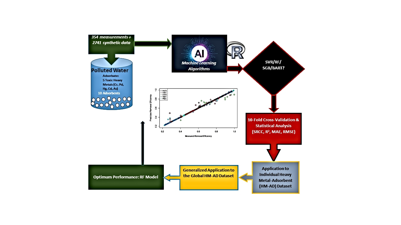
2.3. Dataset
- AD1: Superheated steam-activated granular carbon
- AD2: Ragi husk powder (bio-sorbent)
- AD3: Antep pistachio or Pistacia vera L. (bio-sorbent)
- AD4: Red mud
- AD5: Synthesized functional polydopamine@Fe3O4 nanocomposite (PDA@Fe3O4)
- AD6: Eucalyptus leaves (bio-sorbent)
- AD7: Spirulina (Arthospira) maxima (bio-sorbent)
- AD8: Spirulina (Arthospira) indica (bio-sorbent)
- AD9: Spirulina (Arthospira) platensis (bio-sorbent)
- AD10: Reduced graphene oxide-supported nanoscale zero-valent iron (nZVI/rGO) composites
- AD11: Cupric oxide nanoparticles (CuONPs) prepared with Tamarindus indica pulp extract
- AD12: Cerium hydroxylamine hydrochloride (Ce-HAHCl)
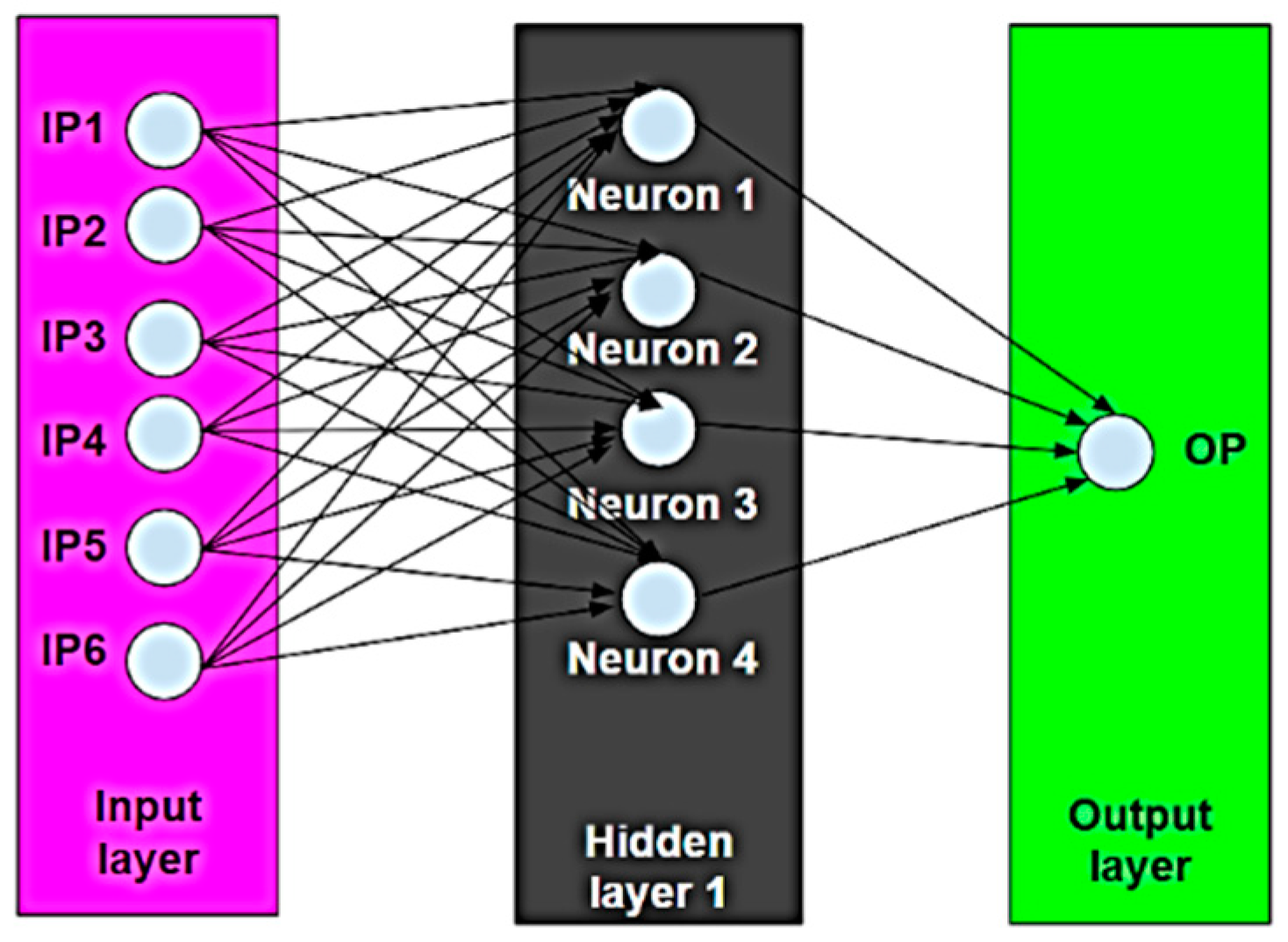
- IP1: Operating temperature, T (°C)
- IP2: Initial pH (-)
- IP3: Initial concentration (mg/L)
- IP4: Contact time (min)
- IP5: Adsorbent dosage (mg)
- IP6: Agitator speed (rpm)
- OP: Removal efficiency (%)
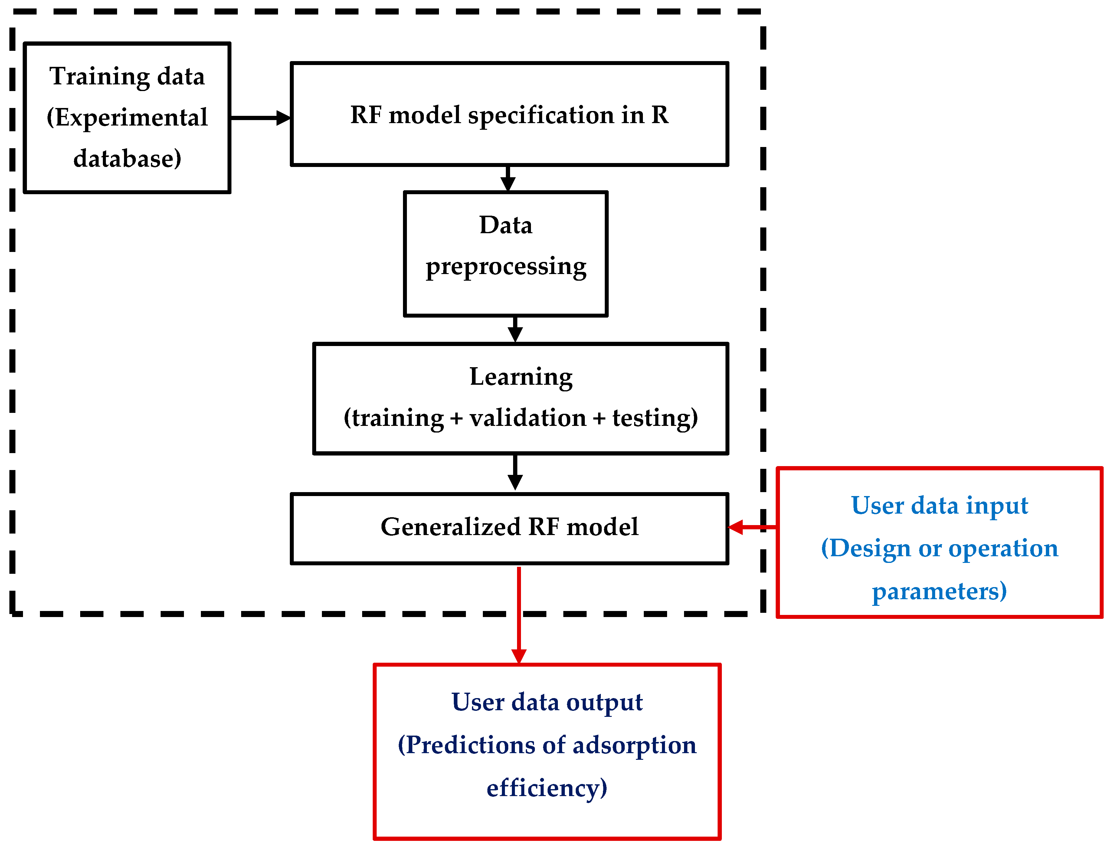
2.4. MLA Modeling
2.4.1. Data Interpolation
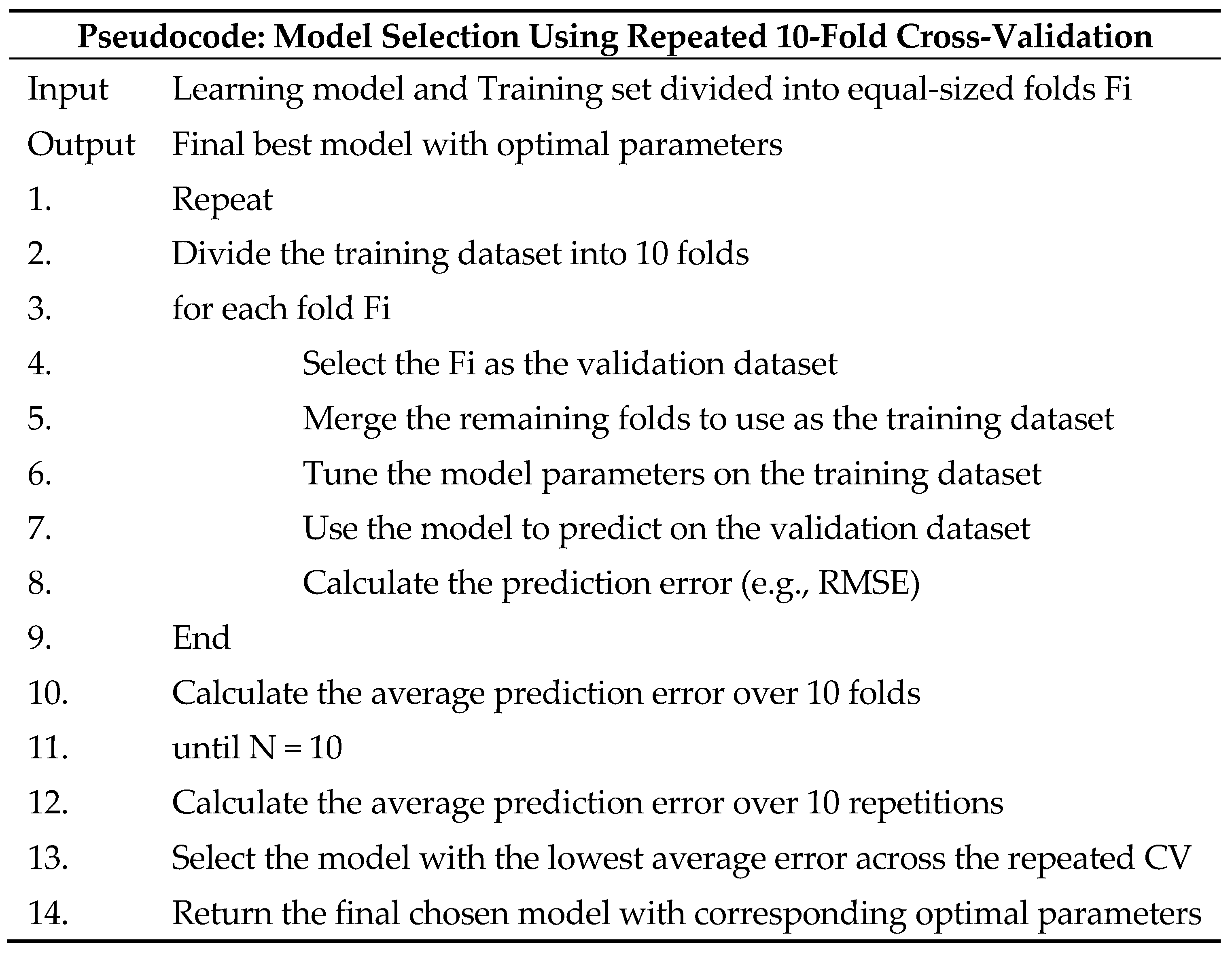
2.4.2. Parameter Optimization and Model Selection
Individual Metal
Comprehensive Dataset
2.5. Computing Framework
3. Results
3.1. ML Model Evaluation for Individual Dataset
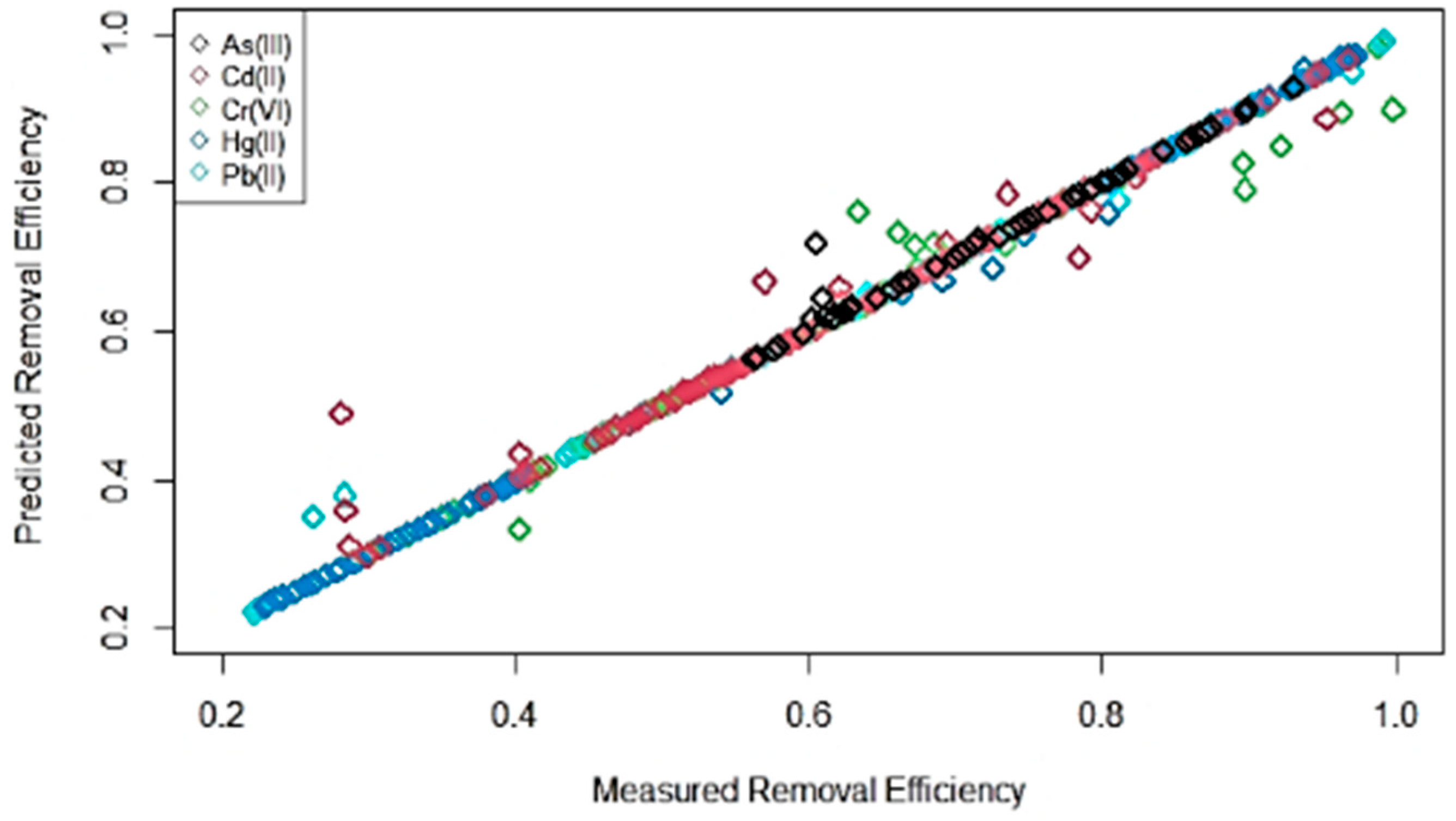
3.2. ML Model Evaluation for Combined Dataset
4. Discussion
5. Conclusions
Author Contributions
Funding
Acknowledgments
Conflicts of Interest
References
- Hegazi, H.A. Removal of heavy metals from wastewater using agricultural and industrial wastes as adsorbents. HBRC J. 2013, 9, 276–282. [Google Scholar] [CrossRef] [Green Version]
- Gupta, V.K.; Gupta, M.; Sharma, S. Process development for the removal of lead and chromium from aqueous solutions using red mud—An aluminium industry waste. Water Res. 2001, 35, 1125–1134. [Google Scholar] [CrossRef]
- Kumar, P.S.; Saravanan, A. Sustainable wastewater treatments in textile sector. In Sustainable Fibres and Textiles; Muthu, S.S., Ed.; Woodhead Publishing: Cambridge, UK, 2017; pp. 323–346. [Google Scholar] [CrossRef]
- Peng, B.; Fang, S.; Tang, L.; Ouyang, X.; Zeng, G. Nanohybrid Materials Based Biosensors for Heavy Metal Detection. In Micro and Nano Technologies, Nanohybrid and Nanoporous Materials for Aquatic Pollution Control; Tang, L., Deng, Y., Wang, J., Wang, J., Zeng, G., Eds.; Elsevier: Amsterdam, The Netherlands, 2019; pp. 233–264. [Google Scholar] [CrossRef]
- Tasharrofi, S.; Hassani, S.S.; Taghdisian, H.; Sobat, Z. Environmentally friendly stabilized nZVI-composite for removal of heavy metals. In New Polymer Nanocomposites for Environmental Remediation; Hussain, C.M., Mishra, A.K., Eds.; Elsevier: Amsterdam, The Netherlands, 2018; pp. 623–642. [Google Scholar] [CrossRef]
- Rhouati, A.; Marty, J.L.; Vasilescu, A. Metal Nanomaterial-Assisted Aptasensors for Emerging Pollutants Detection. In Advanced Nanomaterials; Nikolelis, D.P., Nikoleli, G.P., Eds.; Elsevier: Amsterdam, The Netherlands, 2018; pp. 193–231. [Google Scholar] [CrossRef]
- Atieh, M.A.; Ji, Y.; Kochkodan, V. Metals in the Environment: Toxic Metals Removal. Bioinorg. Chem. Appl. 2017, 2017, 4309198. [Google Scholar] [CrossRef] [PubMed]
- Jin, L.; Zhang, G.; Tian, H. Current state of sewage treatment in China. Water Res. 2014, 66, 85–98. [Google Scholar] [CrossRef] [PubMed]
- Lau, Y.J.; Khan, F.S.A.; Mubarak, N.M.; Lau, S.Y.; Chua, H.B.; Khalid, M.; Abdullah, E.C. Functionalized carbon nanomaterials for wastewater treatment. In Micro and Nano Technologies, Industrial Applications of Nanomaterials; Thomas, S., Grohens, Y., Pottathara, Y.B., Eds.; Elsevier: Amsterdam, The Netherlands, 2019; pp. 283–311. [Google Scholar] [CrossRef]
- Järup, L. Hazards of heavy metal contamination. Br. Med. Bull. 2003, 68, 167–182. [Google Scholar] [CrossRef] [PubMed] [Green Version]
- Khan, S.; Cao, Q.; Zheng, Y.M.; Huang, Y.Z.; Zhu, Y.G. Health risks of heavy metals in contaminated soils and food crops irrigated with wastewater in Beijing, China. Environ. Pollut. 2008, 152, 686–692. [Google Scholar] [CrossRef] [PubMed]
- Schmidt, S.A.; Gukelberger, E.; Hermann, M.; Fiedler, F.; Großmann, B.; Hoinkis, J.; Ghosh, A.; Chatterjee, D.; Bundschuh, J. Pilot study on arsenic removal from groundwater using a small-scale reverse osmosis system towards sustainable drinking water production. J. Hazard. Mater. 2016, 318, 671–678. [Google Scholar] [CrossRef]
- Fu, F.; Wang, Q. Removal of heavy metal ions from wastewaters: A review. J. Environ. Manage. 2011, 92, 407–418. [Google Scholar] [CrossRef]
- Saleh, T.A.; Sarı, A.; Tuzen, M. Optimization of parameters with experimental design for the adsorption of mercury using polyethylenimine modified activated carbon. J. Environ. Chem. Eng. 2017, 5, 1079–1088. [Google Scholar] [CrossRef]
- Benhammou, A.; Yaacoubi, A.; Nibou, L.; Tanouti, B. Adsorption of metal ions onto Moroccan stevensite: Kinetic and isotherm studies. J. Colloid Interface Sci. 2005, 282, 320–326. [Google Scholar] [CrossRef]
- Geyikçi, F.; Kılıç, E.; Çoruh, S.; Elevli, S. Modelling of lead adsorption from industrial sludge leachate on red mud by using RSM and ANN. Chem. Eng. J. 2012, 183, 53–59. [Google Scholar] [CrossRef]
- Wang, S.; Peng, Y. Natural zeolites as effective adsorbents in water and wastewater treatment. Chem. Eng. J. 2010, 156, 11–24. [Google Scholar] [CrossRef]
- Perrich, J.R. Activated Carbon Adsorption for Wastewater Treatment; Fla: Boca Raton, FL, USA; CRC Press: Chicago, IL, USA, 2018. [Google Scholar] [CrossRef]
- Halder, G.; Dhawane, S.; Barai, P.K.; Das, A. Optimizing chromium (VI) adsorption onto superheated steam activated granular carbon through response surface methodology and artificial neural network. Environ. Prog. Sustain. 2015, 34, 638–647. [Google Scholar] [CrossRef]
- Abbas, A.; Al-Amer, A.M.; Laoui, T.; Al-Marri, M.J.; Nasser, M.S.; Khraisheh, M.; Atieh, M.A. Heavy metal removal from aqueous solution by advanced carbon nanotubes: Critical review of adsorption applications. Sep. Purif. Technol. 2016, 157, 141–161. [Google Scholar] [CrossRef]
- Davodi, B.; Ghorbani, M.; Jahangiri, M. Adsorption of mercury from aqueous solution on synthetic polydopamine nanocomposite based on magnetic nanoparticles using Box–Behnken design. J. Taiwan Inst. Chem. Engrs. 2017, 80, 363–378. [Google Scholar] [CrossRef]
- Fan, M.; Li, T.; Hu, J.; Cao, R.; Wei, X.; Shi, X.; Ruan, W. Artificial neural network modeling and genetic algorithm optimization for cadmium removal from aqueous solutions by reduced graphene oxide-supported nanoscale zero-valent iron (nZVI/rGO) composites. Materials 2017, 10, 544. [Google Scholar] [CrossRef]
- Singh, D.K.; Verma, D.K.; Singh, Y.; Hasan, S.H. Preparation of CuO nanoparticles using Tamarindus indica pulp extract for removal of As (III): Optimization of adsorption process by ANN-GA. J. Environ. Chem. Eng. 2017, 5, 1302–1318. [Google Scholar] [CrossRef]
- Peng, W.; Li, H.; Liu, Y.; Song, S. A review on heavy metal ions adsorption from water by graphene oxide and its composites. J. Mol. Liq. 2017, 230, 496–504. [Google Scholar] [CrossRef]
- Mandal, S.; Mahapatra, S.S.; Sahu, M.K.; Patel, R.K. Artificial neural network modelling of As (III) removal from water by novel hybrid material. Process Saf. Environ. Prot. 2015, 93, 249–264. [Google Scholar] [CrossRef]
- Minamisawa, M.; Minamisawa, H.; Yoshida, S.; Takai, N. Adsorption behavior of heavy metals on biomaterials. J. Agric. Food Chem. 2004, 52, 5606–5611. [Google Scholar] [CrossRef]
- Krishna, D.; Sree, R.P. Artificial neural network and response surface methodology approach for modeling and optimization of chromium (VI) adsorption from waste water using Ragi husk powder. Indian Chem. Eng. 2013, 55, 200–222. [Google Scholar] [CrossRef]
- Alimohammadi, M.; Saeedi, Z.; Akbarpour, B.; Rasoulzadeh, H.; Yetilmezsoy, K.; Al-Ghouti, M.A.; Khraisheh, M.; McKay, G. Adsorptive removal of arsenic and mercury from aqueous solutions by eucalyptus leaves. Water Air Soil Pollut. 2017, 228, 429. [Google Scholar] [CrossRef]
- Kiran, R.S.; Madhu, G.M.; Satyanarayana, S.V.; Kalpana, P.; Rangaiah, G.S. Applications of Box–Behnken experimental design coupled with artificial neural networks for biosorption of low concentrations of cadmium using Spirulina (Arthrospira) spp. Resour. Effic. Technol. 2017, 3, 113–123. [Google Scholar] [CrossRef]
- Inyang, M.I.; Gao, B.; Yao, Y.; Xue, Y.; Zimmerman, A.; Mosa, A.; Pullammanappallil, P.; Ok, Y.S.; Cao, X. A review of biochar as a low-cost adsorbent for aqueous heavy metal removal. Crit. Rev. Environ. Sci. Technol. 2016, 46, 406–433. [Google Scholar] [CrossRef]
- Zhu, X.; Wang, X.; Ok, Y.S. The application of machine learning methods for prediction of metal sorption onto biochars. J. Hazard. Mater. 2019, 378, 120727. [Google Scholar] [CrossRef] [PubMed]
- Emigdio, Z.; Abatal, M.; Bassam, A.; Trujillo, L.; Juarez-Smith, P.; El Hamzaoui, Y. Modeling the adsorption of phenols and nitrophenols by activated carbon using genetic programming. J. Clean. Prod. 2017, 161, 860–870. [Google Scholar] [CrossRef]
- Febrianto, J.; Kosasih, A.N.; Sunarso, J.; Ju, Y.; Indraswati, N.; Ismadji, S. Equilibrium and kinetic studies in adsorption of heavy metals using biosorbent: A summary of recent studies. J. Hazard. Mater. 2009, 162, 616–645. [Google Scholar] [CrossRef]
- Vithanage, M.; Rajapaksha, A.U.; Dou, X.; Bolan, N.S.; Yang, J.E.; Ok, Y.S. Surface complexation modeling and spectroscopic evidence of antimony adsorption on ironoxide-rich red earth soils. J. Colloid Interface Sci. 2013, 406, 217–224. [Google Scholar] [CrossRef]
- Bhagat, S.K.; Tung, T.M.; Yaseen, Z.M. Development of artificial intelligence for modeling wastewater heavy metal removal: State of the art, application assessment and possible future research. J. Clean. Prod. 2020, 250, 119473. [Google Scholar] [CrossRef]
- Sakizadeh, M. Artificial intelligence for the prediction of water quality index in groundwater systems. Model. Earth Syst. Environ. 2016, 2, 8. [Google Scholar] [CrossRef]
- Hafsa, N.; Al-Yaari, M.; Rushd, S. Prediction of arsenic removal in aqueous solutions with non-neural network algorithms. Can. J. Chem. Eng. 2020, in press. [Google Scholar] [CrossRef]
- Ahmadi, M.; Chen, Z. Machine learning models to predict bottom hole pressure in multi-phase flow in vertical oil production wells. Can. J. Chem. Eng. 2019, 97, 2928–2940. [Google Scholar] [CrossRef]
- Guo, Y.; Bartlett, P.; Shawe-Taylor, J.; Williamson, R. Covering numbers for support vector machines. IEEE Trans. Inf. Theory 2002, 48, 239–250. [Google Scholar] [CrossRef]
- Durbha, S.; King, R.; Younan, N. Support vector machines regression for retrieval of leaf area index from multiangle imaging spectroradiometer. Remote Sens. Environ. 2007, 107, 348–361. [Google Scholar] [CrossRef]
- Omer, G.; Mutanga, O.; Abdel-Rahman, E.; Adam, E. Performance of support vector machines and artificial neural network for mapping endangered tree species using WorldView-2 data in Dukuduku Forest, South Africa. IEEE J. Sel. Top. Appl. Earth Observ. Remote Sens. 2015, 8, 4825–4884. [Google Scholar] [CrossRef]
- Breiman, L. Random forests. Mach. Learn. 2001, 45, 5–32. [Google Scholar] [CrossRef] [Green Version]
- Čeh, M.; Kilibarda, M.; Lisec, A.; Bajat, B. Estimating the performance of random forest versus multiple regression for predicting prices of the apartments. ISPRS Int. J. Geo-Inf. 2018, 7, 168. [Google Scholar] [CrossRef] [Green Version]
- Wei, L.; Yuan, Z.; Zhong, Y.; Yang, L.; Hu, X.; Zhang, Y. An improved gradient boosting regression tree estimation model for soil heavy metal (arsenic) pollution monitoring using hyperspectral remote sensing. Appl. Sci. 2019, 9, 1943. [Google Scholar] [CrossRef] [Green Version]
- Cha, Y.; Kim, Y.; Choi, J.; Sthiannopkao, S.; Cho, K. Bayesian modeling approach for characterizing groundwater arsenic contamination in the Mekong River basin. Chemosphere 2016, 143, 50–56. [Google Scholar] [CrossRef]
- Yetilmezsoy, K.; Demirel, S.; Vanderbei, R.J. Response surface modeling of Pb (II) removal from aqueous solution by Pistacia vera L.: Box–Behnken experimental design. J. Hazard. Mater. 2009, 171, 551–562. [Google Scholar] [CrossRef]
- Podder, M.S.; Majumder, C.B. The use of artificial neural network for modelling of phycoremediation of toxic elements As (III) and As (V) from wastewater using Botryococcus braunii. Spectrochim. Acta A 2016, 155, 130–145. [Google Scholar] [CrossRef]
- Won, W.; Lee, K. Adaptive predictive collocation with a cubic spline interpolation function for convection-dominant fixed-bed processes: Application to a fixed-bed adsorption process. Chem. Eng. J. 2011, 166, 240–248. [Google Scholar] [CrossRef]
- Aguilera, A.; Morillo, A. Comparative study of different B-spline approaches for functional data. Math. Comput. Model. 2013, 58, 1568–1579. [Google Scholar] [CrossRef]
- R Core Team. R: A Language and Environment for Statistical Computing; R Foundation for Statistical Computing: Vienna, Austria, 2020; Available online: https://www.R-project.org/ (accessed on 20 September 2020).
- Rodriguez, J.D.; Perez, A.; Lozano, J.A. Sensitivity analysis of k-fold cross validation in prediction error estimation. IEEE PAMI 2009, 32, 569–575. [Google Scholar] [CrossRef]


| Reference | HM | AD | Experimental Parameters | Modeling Methodology | |||
|---|---|---|---|---|---|---|---|
| Variable Inputs | Fixed Inputs | Output | Data Points | ||||
| [19] | Cr(VI) | AD1 | IP1 IP2 IP3 IP4 IP5 | IP6 | OP | 36 | - RSM: R2 = 0.9986 - ANN: R2 = 0.9911 |
| [27] | Cr(VI) | AD2 | IP2 IP3 IP5 | IP1 IP4 IP6 | 16 | - ANN: R2 = 0.996 - RSM: R2 = 0.993 | |
| [46] | Pb(II) | AD3 | IP2 IP3 IP4 | IP1 IP5 IP6 | 17 | - RSM: R2 = 0.98383 | |
| [16] | Pb(II) | AD4 | IP2 IP4 IP5 | IP1 IP3 IP6 | 15 | - ANN: R2 = 0.898 - RSM: R2 = 0.672 | |
| [21] | Hg(II) | AD5 | IP2 IP3 IP4 | IP1 IP5 IP6 | OP | 15 | - LI: R2 = 0.991 - FI: R2 = 0.989 - RSM: R2 = 0.9871 |
| [28] | Hg(II) | AD6 | IP2 IP3 IP4 IP5 | IP1 IP6 | 30 | - RSM: R2 = 0.984 - FI: R2 = 0.9849 - LI: R2 = 0.9802 - DRI: R2 = 0.9293 - TI: R2 = 0.8769 | |
| [29] | Cd(II) | AD7 | IP2 IP3 IP5 IP6 | IP1 IP4 | 27 | - FI: R2 = 0.998 - LI: R2 = 0.969 - ANN: R2 = 0.965 - RSM: R2 = 0.760 | |
| Cd(II) | AD8 | 27 | - FI: R2 = 0.994 - ANN: R2 = 0.967 - RSM: R2 = 0.962 - LI: R2 = 0.953 | ||||
| Cd(II) | AD9 | 27 | - ANN: R2 = 0.9955 - FI: R2 = 0.979 - RSM: R2 = 0.974 - LI: R2 = 0.967 | ||||
| [22] | Cd(II) | AD10 | IP1 IP2 IP3 IP4 | IP5 IP6 | 29 | - ANN: R2 = 0.9999 - LI: R2 = 0.9909 - FI: R2 = 0.9852 - RSM: R2 = 0.9826 - DRI: R2 = 0.8226 | |
| [23] | As(III) | AD11 | IP1 IP2 IP3 IP5 | IP4 IP6 | 31 | - ANN: R2 = 0.9994 - LI: R2 = 0.997 - FI: R2 = 0.805 | |
| [25] | As(III) | AD12 | IP1 IP2 IP3 IP4 IP5 IP6 | - | 105 | - ANN: R2 = 0.975 | |
| Parameter (Unit) | Average | Maximum | Minimum | Standard Deviation | HM-AD |
|---|---|---|---|---|---|
| IP1 (°C) | 25.0 | 48.8 | 1.2 | 9.4 | Cr(VI)-AD1 |
| IP2 (-) | 6.0 | 10.8 | 1.2 | 1.9 | |
| IP3 (mg/L) | 150.0 | 268.9 | 31.1 | 47.0 | |
| IP4 (min) | 50.0 | 73.8 | 26.2 | 9.4 | |
| IP5 (mg) | 1.2 | 2.2 | 0.3 | 0.4 | |
| IP6 (rpm) | 150.0 | 150.0 | 150.0 | 0.0 | |
| OP (%) | 71.2 | 96.3 | 39.7 | 10.6 | |
| IP1 (°C) | 25.0 | 25.0 | 25.0 | 0.0 | Cr(VI)-AD2 |
| IP2 (-) | 2.0 | 3.0 | 1.0 | 0.8 | |
| IP3 (mg/L) | 19.3 | 25.0 | 2.0 | 4.9 | |
| IP4 (min) | 120.0 | 120.0 | 120.0 | 0.0 | |
| IP5 (mg) | 3.9 | 60.9 | 1.6 | 10.6 | |
| IP6 (rpm) | 180.0 | 180.0 | 180.0 | 0.0 | |
| OP (%) | 67.0 | 72.7 | 59.2 | 4.0 | |
| IP1 (°C) | 30.0 | 30.0 | 30.0 | 0.0 | Pb(II)-AD3 |
| IP2 (-) | 3.8 | 5.5 | 2.0 | 1.2 | |
| IP3 (mg/L) | 27.5 | 50.0 | 5.0 | 17.8 | |
| IP4 (min) | 62.5 | 120.0 | 5.0 | 45.5 | |
| IP5 (mg) | 1000.0 | 1000.0 | 1000.0 | 0.0 | |
| IP6 (rpm) | 250.0 | 250.0 | 250.0 | 0.0 | |
| OP (%) | 76.0 | 97.3 | 26.5 | 22.5 | |
| IP1 (°C) | 23.0 | 23.0 | 23.0 | 0.0 | Pb(II)-AD4 |
| IP2 (-) | 5.0 | 7.0 | 3.0 | 1.5 | |
| IP3 (mg/L) | 32.1 | 32.1 | 32.1 | 0.0 | |
| IP4 (min) | 32.5 | 60.0 | 5.0 | 20.8 | |
| IP5 (mg) | 5.6 | 10.0 | 1.3 | 3.3 | |
| IP6 (rpm) | 150.0 | 150.0 | 150.0 | 0.0 | |
| OP (%) | 80.6 | 96.8 | 38.8 | 20.9 | |
| IP1 (°C) | 20.0 | 20.0 | 20.0 | 0.0 | Hg(II)-AD5 |
| IP2 (-) | 4.0 | 7.0 | 1.0 | 2.3 | |
| IP3 (mg/L) | 60.0 | 100.0 | 20.0 | 30.2 | |
| IP4 (min) | 240.0 | 420.0 | 60.0 | 136.1 | |
| IP5 (mg) | 10.0 | 10.0 | 10.0 | 0.0 | |
| IP6 (rpm) | 400.0 | 400.0 | 400.0 | 0.0 | |
| OP (%) | 32.7 | 41.0 | 20.5 | 6.3 | |
| IP1 (°C) | 25.0 | 25.0 | 25.0 | 0.0 | Hg(II)-AD6 |
| IP2 (-) | 6.0 | 9.0 | 3.0 | 1.1 | |
| IP3 (mg/L) | 2.7 | 3.9 | 0.5 | 0.5 | |
| IP4 (min) | 47.5 | 90.0 | 5.0 | 15.8 | |
| IP5 (mg) | 1.5 | 2.5 | 0.5 | 0.3 | |
| IP6 (rpm) | 120.0 | 120.0 | 120.0 | 0.0 | |
| OP (%) | 92.6 | 94.7 | 78.5 | 4.2 | |
| IP1 (°C) | 25.0 | 25.0 | 25.0 | 0.0 | Cd(II)-AD7 |
| IP2 (-) | 7.0 | 8.0 | 6.0 | 0.7 | |
| IP3 (mg/L) | 0.0 | 0.0 | 0.0 | 0.0 | |
| IP4 (min) | 6.0 | 6.0 | 6.0 | 0.0 | |
| IP5 (mg) | 0.2 | 0.2 | 0.1 | 0.0 | |
| IP6 (rpm) | 14.0 | 16.0 | 12.0 | 1.4 | |
| OP (%) | 62.3 | 73.3 | 56.6 | 3.8 | |
| IP1 (°C) | 25.0 | 25.0 | 25.0 | 0.0 | Cd(II)-AD8 |
| IP2 (-) | 7.0 | 8.0 | 6.0 | 0.7 | |
| IP3 (mg/L) | 0.0 | 0.0 | 0.0 | 0.0 | |
| IP4 (min) | 6.0 | 6.0 | 6.0 | 0.0 | |
| IP5 (mg) | 0.2 | 0.2 | 0.1 | 0.0 | |
| IP6 (rpm) | 14.0 | 16.0 | 12.0 | 1.4 | |
| OP (%) | 66.2 | 79.2 | 58.2 | 5.7 | |
| IP1 (°C) | 25.0 | 25.0 | 25.0 | 0.0 | Cd(II)-AD9 |
| IP2 (-) | 7.0 | 8.0 | 6.0 | 0.7 | |
| IP3 (mg/L) | 0.0 | 0.0 | 0.0 | 0.0 | |
| IP4 (min) | 6.0 | 6.0 | 6.0 | 0.0 | |
| IP5 (mg) | 0.2 | 0.2 | 0.1 | 0.0 | |
| IP6 (rpm) | 14.0 | 16.0 | 12.0 | 1.4 | |
| OP (%) | 69.9 | 82.5 | 61.8 | 5.6 | |
| IP1 (°C) | 30.0 | 40.0 | 20.0 | 6.5 | Cd(II)-AD10 |
| IP2 (-) | 6.0 | 7.0 | 5.0 | 0.7 | |
| IP3 (mg/L) | 30.0 | 40.0 | 20.0 | 6.5 | |
| IP4 (min) | 20.0 | 30.0 | 10.0 | 6.5 | |
| IP5 (mg) | 30.0 | 30.0 | 30.0 | 0.0 | |
| IP6 (rpm) | 200.0 | 200.0 | 200.0 | 0.0 | |
| OP (%) | 60.1 | 77.3 | 44.3 | 8.7 | |
| IP1 (°C) | 40.0 | 60.0 | 20.0 | 8.9 | As(III)-AD11 |
| IP2 (-) | 7.0 | 12.0 | 2.0 | 2.2 | |
| IP3 (mg/L) | 1000.0 | 1900.0 | 100.0 | 402.5 | |
| IP4 (min) | 270.0 | 270.0 | 270.0 | 0.0 | |
| IP5 (mg) | 75.0 | 135.0 | 15.0 | 26.8 | |
| IP6 (rpm) | 100.0 | 100.0 | 100.0 | 0.0 | |
| OP (%) | 76.2 | 92.7 | 48.2 | 12.3 | |
| IP1 (°C) | 38.5 | 60.0 | 20.0 | 16.3 | As(III)-AD12 |
| IP2 (-) | 7.5 | 10.0 | 4.0 | 2.4 | |
| IP3 (mg/L) | 23.2 | 50.0 | 10.0 | 15.7 | |
| IP4 (min) | 62.3 | 90.0 | 30.0 | 23.4 | |
| IP5 (mg) | 7733.3 | 10,000.0 | 6000.0 | 1761.0 | |
| IP6 (rpm) | 162.1 | 180.0 | 120.0 | 23.8 | |
| OP (%) | 76.6 | 98.9 | 50.0 | 13.9 | |
| Overall statistics | |||||
| IP1 (°C) | 30.0 | 60.0 | 1.2 | 11.9 | Cr(VI)-AD1 Cr(VI)-AD2 Pb(II)-AD3 Pb(II)-AD4 Hg(II)-AD5 Hg(II)-AD6 Cd(II)-AD7 Cd(II)-AD8 Cd(II)-AD9 Cd(II)-AD10 As(II)-AD11 As(II)-AD12 |
| IP2 (-) | 6.0 | 12.0 | 1.0 | 2.3 | |
| IP3 (mg/L) | 102.6 | 1900.0 | 0.0 | 261.1 | |
| IP4 (min) | 78.7 | 420.0 | 5.0 | 78.9 | |
| IP5 (mg) | 1737.0 | 10,000.0 | 0.0 | 3281.4 | |
| IP6 (rpm) | 178.7 | 800.0 | 12.0 | 178.1 | |
| OP (%) | 68.1 | 98.9 | 0.9 | 21.3 | |
| Model | Hyperparameter Names | R Package |
|---|---|---|
| Random Forest | [mtry] | randomForest |
| SVR–RBF Kernel | [sigma, C] | kernlab |
| SVR–Polynomial Kernel | [degree, scale, C] | kernlab |
| Stochastic Gradient Boosting | [n.trees, interaction.depth] | gbm |
| Bayesian Additive Regression | [num_trees] | bartMachine |
| Combined Dataset (Five Metals) | Percentage | No. Data Points |
|---|---|---|
| Training | 80% | 2476 |
| Test | 20% | 619 |
| Total | 100% | 3095 |
| Metal | Algorithm | Performance | |||
|---|---|---|---|---|---|
| MAE | RMSE | SPcorr | R2 | ||
| As (III) 1 | SVR-Poly | 2.42 | 5.43 | 0.91 | 0.84 |
| Stochastic Gradient Boosting | 1.51 | 3.13 | 0.97 | 0.93 | |
| SVR-RBF | 2.41 | 5.30 | 0.92 | 0.84 | |
| Random Forest | 1.36 | 3.53 | 0.96 | 0.93 | |
| Bayesian Additive Regression Tree | 1.33 | 4.18 | 0.98 | 0.97 | |
| As (III) 2 | SVR-Poly | 3.32 | 6.08 | 0.89 | 0.80 |
| Stochastic Gradient Boosting | 2.71 | 5.67 | 0.90 | 0.81 | |
| SVR-RBF | 3.38 | 5.89 | 0.89 | 0.80 | |
| Random Forest | 2.72 | 5.92 | 0.89 | 0.80 | |
| Bayesian Additive Regression Tree | 2.57 | 5.83 | 0.89 | 0.79 | |
| Metal | Algorithm | Performance | |||
|---|---|---|---|---|---|
| MAE | RMSE | SPcorr | R2 | ||
| Cr(IV) 1 | SVR-Poly | 0.38 | 1.08 | 0.94 | 0.89 |
| Stochastic Gradient Boosting | 1.51 | 3.13 | 0.97 | 0.93 | |
| SVR-RBF | 0.49 | 1.14 | 0.94 | 0.89 | |
| Random Forest | 1.36 | 3.53 | 0.96 | 0.93 | |
| Bayesian Additive Regression Tree | 0.10 | 0.15 | 0.99 | 0.99 | |
| Cr (IV) 2 | SVR-Poly | 2.16 | 3.84 | 0.97 | 0.95 |
| Stochastic Gradient Boosting | 2.04 | 4.80 | 0.96 | 0.92 | |
| SVR-RBF | 1.62 | 3.04 | 0.98 | 0.96 | |
| Random Forest | 1.60 | 4.65 | 0.96 | 0.92 | |
| Bayesian Additive Regression Tree | 1.21 | 4.0 | 0.97 | 0.94 | |
| Metal | Algorithm | Performance | |||
|---|---|---|---|---|---|
| MAE | RMSE | SPcorr | R2 | ||
| Cd (II) 1 | SVR-Poly | 1.06 | 1.77 | 0.97 | 0.95 |
| Stochastic Gradient Boosting | 0.58 | 1.32 | 0.98 | 0.97 | |
| SVR-RBF | 0.95 | 1.39 | 0.98 | 0.97 | |
| Random Forest | 0.66 | 2.00 | 0.96 | 0.92 | |
| Bayesian Additive Regression Tree | 0.65 | 1.60 | 0.99 | 0.98 | |
| Cd (II) 2 | SVR-Poly | 2.44 | 5.42 | 0.96 | 0.92 |
| Stochastic Gradient Boosting | 2.05 | 5.07 | 0.96 | 0.93 | |
| SVR-RBF | 2.0 | 3.59 | 0.98 | 0.97 | |
| Random Forest | 1.63 | 5.18 | 0.96 | 0.92 | |
| Bayesian Additive Regression Tree | 1.16 | 3.22 | 0.98 | 0.97 | |
| Metal | Algorithm | Performance | |||
|---|---|---|---|---|---|
| MAE | RMSE | SPcorr | R2 | ||
| Hg (II) 1 | SVR-Poly | 0.54 | 0.95 | 0.97 | 0.95 |
| Stochastic Gradient Boosting | 0.29 | 0.61 | 0.99 | 0.98 | |
| SVR-RBF | 0.42 | 0.90 | 0.98 | 0.96 | |
| Random Forest | 0.11 | 0.38 | 0.99 | 0.99 | |
| Bayesian Additive Regression Tree | 0.24 | 0.78 | 0.99 | 0.98 | |
| Hg (II) 2 | SVR-Poly | 0.61 | 1.67 | 0.94 | 0.88 |
| Stochastic Gradient Boosting | 0.26 | 0.75 | 0.98 | 0.97 | |
| SVR-RBF | 1.13 | 1.99 | 0.95 | 0.91 | |
| Random Forest | 0.23 | 0.85 | 0.95 | 0.97 | |
| Bayesian Additive Regression Tree | 0.14 | 0.30 | 0.99 | 0.99 | |
| Metal | Algorithm | Performance | |||
|---|---|---|---|---|---|
| MAE | RMSE | SPcorr | R2 | ||
| Pb (II) 1 | SVR-Poly | 2.29 | 3.47 | 0.98 | 0.97 |
| Stochastic Gradient Boosting | 1.46 | 1.37 | 0.98 | 0.96 | |
| SVR-RBF | 1.96 | 3.59 | 0.98 | 0.97 | |
| Random Forest | 0.92 | 3.14 | 0.98 | 0.96 | |
| Bayesian Additive Regression Tree | 0.61 | 1.37 | 0.99 | 0.99 | |
| Pb (II) 2 | SVR-Poly | 1.13 | 1.99 | 1.0 | 1.0 |
| Stochastic Gradient Boosting | 0.90 | 2.21 | 0.99 | 0.99 | |
| SVR-RBF | 2.29 | 3.47 | 1.0 | 1.0 | |
| Random Forest | 0.18 | 0.42 | 0.99 | 0.99 | |
| Bayesian Additive Regression Tree | 0.69 | 2.78 | 0.99 | 0.99 | |
| Model | Train | Test | ||||||
|---|---|---|---|---|---|---|---|---|
| MAE | RMSE | SPCC | R2 | MAE | RMSE | SPCC | R2 | |
| SVR-Poly | 0.0276 | 0.046 | 0.977 | 0.976 | 0.0278 | 0.052 | 0.972 | 0.970 |
| SGB | 0.0247 | 0.043 | 0.981 | 0.979 | 0.249 | 0.047 | 0.979 | 0.976 |
| SVR-RBF | 0.0267 | 0.043 | 0.981 | 0.978 | 0.0273 | 0.050 | 0.976 | 0.973 |
| RF | 0.004 | 0.015 | 0.997 | 0.997 | 0.007 | 0.033 | 0.989 | 0.988 |
| BART | 0.023 | 0.048 | 0.990 | 0.974 | 0.025 | 0.054 | 0.983 | 0.969 |
Publisher’s Note: MDPI stays neutral with regard to jurisdictional claims in published maps and institutional affiliations. |
© 2020 by the authors. Licensee MDPI, Basel, Switzerland. This article is an open access article distributed under the terms and conditions of the Creative Commons Attribution (CC BY) license (http://creativecommons.org/licenses/by/4.0/).
Share and Cite
Hafsa, N.; Rushd, S.; Al-Yaari, M.; Rahman, M. A Generalized Method for Modeling the Adsorption of Heavy Metals with Machine Learning Algorithms. Water 2020, 12, 3490. https://doi.org/10.3390/w12123490
Hafsa N, Rushd S, Al-Yaari M, Rahman M. A Generalized Method for Modeling the Adsorption of Heavy Metals with Machine Learning Algorithms. Water. 2020; 12(12):3490. https://doi.org/10.3390/w12123490
Chicago/Turabian StyleHafsa, Noor, Sayeed Rushd, Mohammed Al-Yaari, and Muhammad Rahman. 2020. "A Generalized Method for Modeling the Adsorption of Heavy Metals with Machine Learning Algorithms" Water 12, no. 12: 3490. https://doi.org/10.3390/w12123490
APA StyleHafsa, N., Rushd, S., Al-Yaari, M., & Rahman, M. (2020). A Generalized Method for Modeling the Adsorption of Heavy Metals with Machine Learning Algorithms. Water, 12(12), 3490. https://doi.org/10.3390/w12123490