Observation Strategies Based on Singular Value Decomposition for Ocean Analysis and Forecast

Abstract

In this article, we discuss possible observing strategies for a simplified ocean model (Double Gyre (DG)), used as a preliminary tool to understand the observation needs for real analysis and forecasting systems. Observations are indeed fundamental to improve the quality of forecasts when data assimilation techniques are employed to obtain reliable analysis results. In addition, observation networks, particularly in situ observations, are expensive and require careful positioning of instruments. A possible strategy to locate observations is based on Singular Value Decomposition (SVD). SVD has many advantages when a variational assimilation method such as the 4D-Var is available, with its computation being dependent on the tangent linear and adjoint models. SVD is adopted as a method to identify areas where maximum error growth occurs and assimilating observations can give particular advantages. However, an SVD-based observation positioning strategy may not be optimal; thus, we introduce other criteria based on the correlation between points, as the information observed on neighboring locations can be redundant. These criteria are easily replicable in practical applications, as they require rather standard studies to obtain prior information.

1. Introduction

In recent years, there has been a growing demand for oceanographic forecast data [1,2], which comes from different public and private subjects for operational oceanography purposes. This request stimulates the production of reliable predictions of physical and biogeochemical ocean variables to support activities such as search and rescue operations, ocean energy, fisheries, and environmental monitoring and pollution control. Observations play an essential role in operational systems as they also allow evaluating the reliability of predictions. The most important initiative in this context is the Global Ocean Observation System (GOOS), which includes several regional observation components providing data to global and basin-scale operational services, as well as to regional downstream services [3].

Operational oceanographic services both at the basin and regional scales improve their forecast reliability when the model forecast is properly initialized with fields obtained through a data assimilation procedure. Data assimilation (DA) combines observations and models first-guess-weighted by their respective accuracies to obtain the best unbiased estimation of the ocean state. In a DA scheme, the observations correct the trajectory (first guess) according to their influence, which mainly depends on the observation and model error covariance matrices. As a consequence, DA can be useful to better control the error growth of the state trajectory with respect to the real evolution. Furthermore, in the operational practice, a common procedure of initializing a simulation starting with external data (e.g., climatology, objective analysis, model analysis, etc.) requires a spin-up interval during which the solution is not usable. DA schemes as 4D-Var reduce the spin-up effects (keeping a dynamical consistency between analysis and model equations) and also reduce model uncertainties.

Large amounts of data come from satellite observations (mainly Sea Surface Temperature and Sea Surface Height), which have some intrinsic limitations (surface-limited observations, revisiting times). Many parameters are only observable by collecting in situ observations through specific sensor networks that integrate satellite observations with data along the water column and at higher frequencies. The main limitation of in situ observation networks is their high cost for installation and maintenance over time; it is very important, therefore, to design an in situ observing system that maximizes the impact of the observations in the forecast, minimizing the cost.

Ocean models can also be used to evaluate both existing and new observing networks through different methodologies [4]. Observing System Experiments (OSEs) compare analysis obtained by eliminating only a part of the observations with the analysis obtained by assimilating the entire dataset to understand the impact of the omitted observations. Observation System Simulation Experiments (OSSEs) use “synthetic” observations to evaluate the benefit of assimilating observations from instruments/networks not yet installed. Adjoint-based techniques and ensemble-based methods can be used to study observation sensitivities and the impact on assimilated systems, contributing to the design of observing systems [4,5,6].

As different observations have different impacts when they are assimilated in an ocean model, a major problem is designing an observation network that provides data giving the best results (i.e., fewer errors) when they are assimilated. The positioning of the observing system is indeed somehow related to the unstable modes, which deserve more than others to be corrected. Since the fundamental milestone made by Lorenz in 1965 [7], it is well known how the divergence in chaotic systems rises from the unstable directions of the state trajectory where small errors in initial conditions significantly grow, leading to very different final states. This places a time limit to the predictability of the system state, which is usually evaluated by the largest Lyapunov exponents. The assimilation of observations attempts to prolong that time limit [8]. Some significant errors could decay over time, whereas smaller errors could intensely grow and produce a heavy impact on forecast reliability. The growth of the divergence between model evolution and the real state of the system is driven by these unstable directions, rather than by the largest components of the error embedded in the predicting system [9,10]. Indeed, the structure of the fast-growing perturbations is a dynamically evolving field and depends on the flow regime, as it derives from the position of the current state on the attractor and varies over time [7,11,12].

For what concerns observation strategies, we can expect that a suitable positioning of observation devices in areas in which error in the initial condition is fast-growing may better control this growth. Such a choice can be performed on the basis of the study of perturbation growth. Hansen and Smith [13] showed that for sufficiently small errors, observation strategies based on system dynamics produce better results than strategies based on error estimates.

A notable contribution to this field was made by Farrell and Joannou [14,15] in their General Stability Theory (GST) of a dynamical system, in which they extended the traditional modal stability theory to include transient growth processes. The authors identified the decomposition to singular values (SVD) as a suitable tool for treating perturbation growths in geophysical fluid systems. A variation of this method considers the calculation of Hessian singular vectors, which identify the errors in initial conditions that evolve into the largest forecast errors [6].

The existence of large singular values indicates that small errors in the initial background state can grow very rapidly, reducing the system predictability, and the respective singular vectors indicate the areas where disturbances grow faster. Analyzing Singular Vectors (SVs) appears strategic to increase model predictability by giving an indication of where it is more important to reduce errors in initial conditions [6,16].

The application of SVD to select observations has been already tested in a number of studies, mostly related to operational aspects of atmospheric forecasting systems [5,17,18,19,20,21]. A review of observation strategies [22] confirmed the utility of SVD information in choosing the observations to be assimilated. Bergot et al. [23] considered the SVD as a useful tool to identify areas where assimilating even a few observations is able to significantly reduce forecast errors. An important portion of literature about the topic of adaptive observations was originated by the first experimental reference, the so-called Fronts and Atlantic Storm Track Experiment (FASTEX) [24,25,26]. Other experiments were carried out by assimilating additional observations from aircraft in regions characterized by rapidly growing SVs [19,27,28].

In this work, we test some possible observation strategies of a simplified ocean system with the aim of establishing an optimal configuration of an in situ observing network able to reduce forecasting uncertainties through DA. For simplicity, we limit this study to velocity observations. In particular, our goal is to achieve such an optimal configuration using a limited number of observation points, as these may have a significant cost, in order to ensure the greatest possible benefit to an integrated assimilation/forecasting system. The benefit is measured with respect to the short-/medium-range forecast (analysis and forecast cycles of a few days), as required in the operational practice. In order to select the possible observation points, the proposed strategy is based on the SVD and on a maximum correlation among the horizontal velocities, which is traduced into a minimum distance, variable over the model domain. Indeed, we verify that an observation strategy based on SVD may fail if it is not accompanied by other considerations linked to the flow structure, and such a combination of SVD analysis with a correlation analysis can be used to limit redundant observations.

The experiments are carried out by using the ocean model ROMS (Regional Ocean Modelling System, www.myroms.org) [29], which already includes suitable routines for the SVD computation [30]. We perform a set of numerical experiments assimilating different datasets and investigate the effects on model results.

In Section 2, the configuration of the experiment is presented, and in particular, the description of the model, the DA scheme, and the proposed strategy to place in situ observation points.

In Section 3, the results of all experiments are reported; our best strategy is compared to a random localization strategy and also to a selection procedure based on SVD and on a minimum fixed distance among observations.

2. Materials and Methods

2.1. The Model Set-Up

The reference model used in this work is an idealized ocean model, widely known as Double Gyre (DG). Although it is conceptually much simpler than realistic simulations, it is still relevant from an oceanographic point of view. DG simplified dynamics have been used as an idealized case to reproduce the seasonal and interannual oscillations of the large-scale circulation in the ocean, useful for the climate system predictability [30].

This configuration is also used by the ROMS developers [31] as a test case to introduce the functionalities of the tangent linear model and its adjoint. This simplified ocean system is strongly barotropic, and no relevant differences can be found in different vertical layers. The basin has a flat bathymetry 500 m deep with all closed boundaries. The model domain is a large rectangular basin 1000 km in size in the east–west direction and 2000 km in the north–south direction; it is discretized horizontally in 56 × 110 cells and vertically in 4 equally spaced s-levels. The model is forced by a constant zonally uniform wind stress with a positive zonal component at its midaxis, which is inverted to a negative zonal component approaching the northern and southern boundaries, as defined by a sinusoidal function of latitude:

$${\tau }_x=-{\tau }_{0}cos\left(\frac{2\pi y}{L_y}\right)$$

(1)

where ${\tau }_0= 0$.05 N/m² and L_y is the meridional extent of the basin. This particular wind distribution induces two large interacting vortices with a scale of about 1000 km: a subpolar cyclonic gyre and a subtropical anticyclonic gyre, whose stationary depends on the eddy viscosity values.

The model solves the 3D primitive equations in a beta-plane approximation centered at 45° N. Density profiles are defined by an analytically stable profile of the active tracers, as described by Moore et al. [31]. The advection for both 3D momentum and tracers in the horizontal and vertical components is implemented by, respectively, the third-order upstream scheme along constant S-surfaces and the fourth-order centered scheme. Horizontal turbulent processes are parametrized by a harmonic operator whose horizontal eddy viscosity and diffusivity are equal to 160 m²/s. Although forced by a steady wind, the model solution depends on the eddy viscosity value, and circulation passes from a stationary pattern (high eddy viscosity) to an oscillating behavior (low eddy viscosity), with the formation of smaller-scale vortices and the shifting of the main current patterns. In fact, the DG circulation shows a bifurcation [32], corresponding to a critical value of the Reynolds number. For values lower than the critical value, the flow converges quickly to a unique steady solution, whereas for values above the critical value, instabilities occur, and the symmetry of the structure of the subpolar and subtropical cells is broken. The vertical turbulent mixing is parameterized by coefficients of vertical viscosity and diffusion of 1 m²/s; linear bottom friction is introduced with a bottom drag coefficient of 8 × 10⁻⁷ m/s. To ensure model stability, the numerical time steps are set, respectively, to 45 s (barotropic time step) and 900 s (baroclinic time step).

The model is initially started through the steady solution (Figure 1a), obtained by a 20-year-long simulation with a high eddy viscosity, equal to 1280 m²/s, which ensures a steady circulation that is symmetrical with respect to the zonal axis. For the following 10-year run, the eddy viscosity is then decreased to a lower value of 160 m²/s: in this case, the circulation loses symmetry as it becomes unsteady and characterized by meandering where the two original gyres move through the domain with other gyres arising.

For our model experiments we define a couple of independent model runs:

1.

A Nature Run (NR), which is the model initialized by the last snapshot of the 10-year run (Figure 1c). This is considered the true state of the ocean, a virtual reality from which synthetic observations are extracted;

2.

A Free Run (FR) or background, which is the simulation initialized by an initial velocity field obtained by averaging the unsteady solution of the 10-year run (Figure 1b). This represents the common and simplest way to initialize numerical simulations by means of a “climatological” time-averaged solution.

In each experiment, a set of observations is extracted from the NR using the observation strategies discussed below. Such a synthetic dataset includes velocity observations in the form of ocean current profiles at a frequency of 15 min, which are assimilated using the FR as the background, thus producing an analysis. In real ocean-observing systems, such kinds of observations are normally taken by means of Acoustic Doppler Current Profilers (ADCPs). The analysis is performed in a 5-day assimilation window that provides initial conditions to a subsequent 5-day forecast.

The positions of observation instruments are fixed in each experiment and chosen by adopting three different strategies: (1) randomly, (2) in the area of maximum dominant singular vectors and imposing a minimum distance among the positions, and (3) in the area of maximum dominant singular vectors, imposing a maximum limit of correlation between the velocity time series in each position. For what concerns the first set of experiments (random positioning), the positions are obtained by the rand function in MATLAB©, assuming a minimum distance is equal to the grid cell size (in this case, around 18 km). To reduce the dependence of the results on a particular random spatial configuration, we repeat each experiment by assimilating different datasets characterized by the same number of (virtual) observation instruments. Finally, to assess the selection procedure for different hydrodynamic states, the assimilation test is repeated in different time windows.

The assimilation of synthetic observations is executed through the incremental formulation of the 4D-Var based on the Lanczos algorithm (ROMS-IS4DVar). In such a procedure, the increments to add to the control vector to minimize the cost function are computed iteratively [5]. The control vector corresponds to the initial state, so only the initial conditions were adjusted by assimilating data.

A maximum number of 10 inner loops and 2 outer loops are set up, and the assimilation process stops when the minimization of the cost function gradient reaches a given tolerance that we set equals 10⁻⁴, as we verified that this limit is sufficiently adequate for convergence. The presence of observation errors is considered in the observation error matrix as we assume implicitly that observations are affected by an error of 0.01 m/s.

The background error covariance matrix B_x is factorized by means of the univariate correlation matrix C, the diagonal matrix of the prior error standard deviations Σ_x, and the multivariate balance operator K_b, as described in [5]:

$$B_x=K_b{\mathsf{\Sigma }}_{x}C{\mathsf{\Sigma }}_x^T{K}_b^T.$$

(2)

The background error standard deviation Σ_x is defined by using the standard deviation of the state variable fields during the 10-year-long (unsteady) simulation, a period long enough to compute meaningful circulation statistics.

The correlation matrix C is in turn factorized by a diagonal matrix of grid box volumes W, a horizontal and vertical correlation function model L_h and L_v, and a matrix of normalization coefficients Λ, as:

$$C=\mathsf{\Lambda }{L}_v^{1/2}{L}_h^{1/2}{W}^{-1}{L}_h^{T/2}{L}_v^{T/2}{\mathsf{\Lambda }}^T.$$

(3)

The normalization coefficients are used to ensure that the diagonal elements of the associated correlation matrix C are equal to unity and they are computed through the so-called “exact method,” in which the horizontal and vertical isotropic decorrelation scales imposed equal 30 km and 100 m, respectively, for all the state variables.

2.2. Observation Strategies

The proposed criteria for identifying the most suitable positions to install observation instruments join two requirements: (a) finding areas characterized by high values of the dominant SVs; (b) imposing a maximum limit to the correlation between the velocity time series at the observation points.

For what concerns the first requirement, we resort to the Singular Value Decomposition (SVD) of the tangent propagator to identify the directions of maximum error growth in a given time interval, according to the Generalized Stability Theory (GST) by Farrell and Ioannou [14,15] for nonautonomous systems. SVD decomposes the matrix L (in this study, it is the tangent propagator) in three matrices that satisfy LV = US [33]. The matrices V and U are formed by the eigenvectors of L^TL and LL^T, respectively, which are autonomous and symmetric for construction. Therefore, their eigenvectors form two orthogonal bases of the domain space and the range space, respectively. For this property, any disturbance at the initial time can be written as a linear combination of the initial singular vectors in the domain space, whereas its evolution can be written as a linear combination of the final singular vectors in the range space. Furthermore, the eigenvalues are the same for both matrices, L^TL and LL^T, and are called singular values; their square root corresponds to the growth factor of the relative initial singular vector, as they are transformed by L. Therefore, the growth rate of all the perturbations is confined by the fastest-growing singular mode, characterized the higher singular value. The dominant initial singular vector defines the direction of maximum growth error in the interval [t₁,t₂]. This calculation allows us to assess the fastest-growing disturbance among all those possible during a given finite time interval, called optimization time. The SVD computation is controlled by two main parameters: the norm, by which the growth of the singular vectors is evaluated, and the optimization time. The dominant initial singular vector is calculated as the singular vector that maximizes a norm at the final time of the interval, as adopting different norms leads to different SVs. In most oceanographic studies, the norm used is the total energy, the same we apply in this work, although other norms have been used depending on the particular aim, such as kinetic energy, enstrophy, and the Hessian norm [5,6,17,33,34]. More details on the SVD can be found in Farrell and Ioannou [14,15].

The number of singular modes of the system is of the order of 10⁵, equivalent to the dimension of the model state. The leading singular vectors are computed in ROMS through the Lanczos algorithm [35] by integrating the tangent linear model forward in time and the adjoint model backward in time a sufficient number of times for the convergence of the algorithm [31].

The SVD is applied with respect to the tangent model of the free-run circulation starting from the climatological state so it is the same for all the time windows. The 200 dominant SVs are computed for different optimization times (5, 10, 20, and 60 days). In Figure 2, the singular values computed with optimization times of 5 and 60 days are reported as examples, and we see that the choice of limiting the calculation to the first 200 SVs, containing the main information on the perturbation evolution, is adequate as it also avoids the computation of a huge number of SVs.

Figure 3 shows the sum of projections onto the horizontal surface velocity components of all the dominant initial singular vectors (upper maps) and the dominant final vectors (bottom maps), weighted with the corresponding singular values. SVs and singular values are computed from the free run by considering different optimization time (T_op) of 5, 10, 20, and 60 days. The structures of the initial and final singular vectors computed on a short T_op are similar to each other and concentrated near the convergence of the currents along the western side, where the two branches of the currents merge and change their direction (from meridional to zonal).

The difference between the initial and the final singular vectors maps grows for increasing optimization times, as well as the singular values (Figure 2). The perturbations computed for 60 days evolve much more than those computed over a shorter period, in agreement with the higher singular values obtained for larger optimization times. However, significantly large singular values, even for the 5-day optimization window, are due to the fact that the initial period of the background run is subject to a strong tendency to change the circulation structure, especially close to the convergence area. Indeed, the simulation starts from the climatological state (Figure 1b) and the circulation is subject to strong variations which are concentrated in the central–western area.

Concerning the second requirement, we set a minimum distance among observations, defined on the basis of a maximum correlation between the time series of model velocities at the observation positions themselves.

The need to impose a minimum distance among in situ observations arises from the typical structure of the dominant singular vectors quite concentrated in specific areas. The highest values of the SV component on the surface velocity are strictly localized in the middle of the western boundary where the ascending and descending currents converge (Figure 2). On the one hand, it is crucial to control such areas of maximum error growth with sufficient detail. On the other hand, having too many observation points concentrated in this part would not give a strong benefit to the analysis since horizontal velocities in this area can be strongly correlated to each other. Therefore, a procedure only based on SV would lead to select too dense instrument positioning. Hence, some experiments are realized imposing a fixed minimum distance between the observation points, but this method does not avoid choosing sampling points excessively correlated. Moreover, we expect for most hydrodynamic fields of interest, the correlation between points is not homogeneous on the whole domain, as well as the suitable minimum distance among observations. This correlation is computed by the following steps:

(1)

For each grid cell (i, j) we compute the spatial correlation of both the u and v velocity components with respect to all of the other grid cells (h, l), with i ≠ h and j ≠ l, and then we take the norm of the matrix:

$$\left|\begin{array}{cc}〈u_{ij}{u}_{hl}〉& 〈v_{ij}{u}_{hl}〉\\ 〈u_{ij}{v}_{hl}〉& 〈v_{ij}{v}_{hl}〉\end{array}\right|.$$

(4)

Each cell is associated with a single normalized correlation map, whose values range between 0 (uncorrelated grid cells) and 1 (perfectly correlated grid cells).

(2)

A maximum value for such normalized correlation is imposed as a threshold to calculate for each grid cell the averaged distance beyond which the correlation is lower than the chosen threshold. In this way, all correlation maps for each grid cell can be transformed into a single map of distances. This map of minimum distances among in situ observation points is computed as the mean radius inside which the correlation of the variable of interest is higher than the imposed correlation threshold.

Figure 4 shows the map of distances used in this study (in km), computed by imposing a maximum correlation of the time series of velocities equal to 0.6. Note that distances are never too small (in this case, >100 km) and they increase moving away from the critical area of convergence.

3. Results

As described in the previous sections, we test three different observation strategies applied to an idealized ocean model (DG) to identify the observation network configuration, which gives rise to the best analysis and forecast.

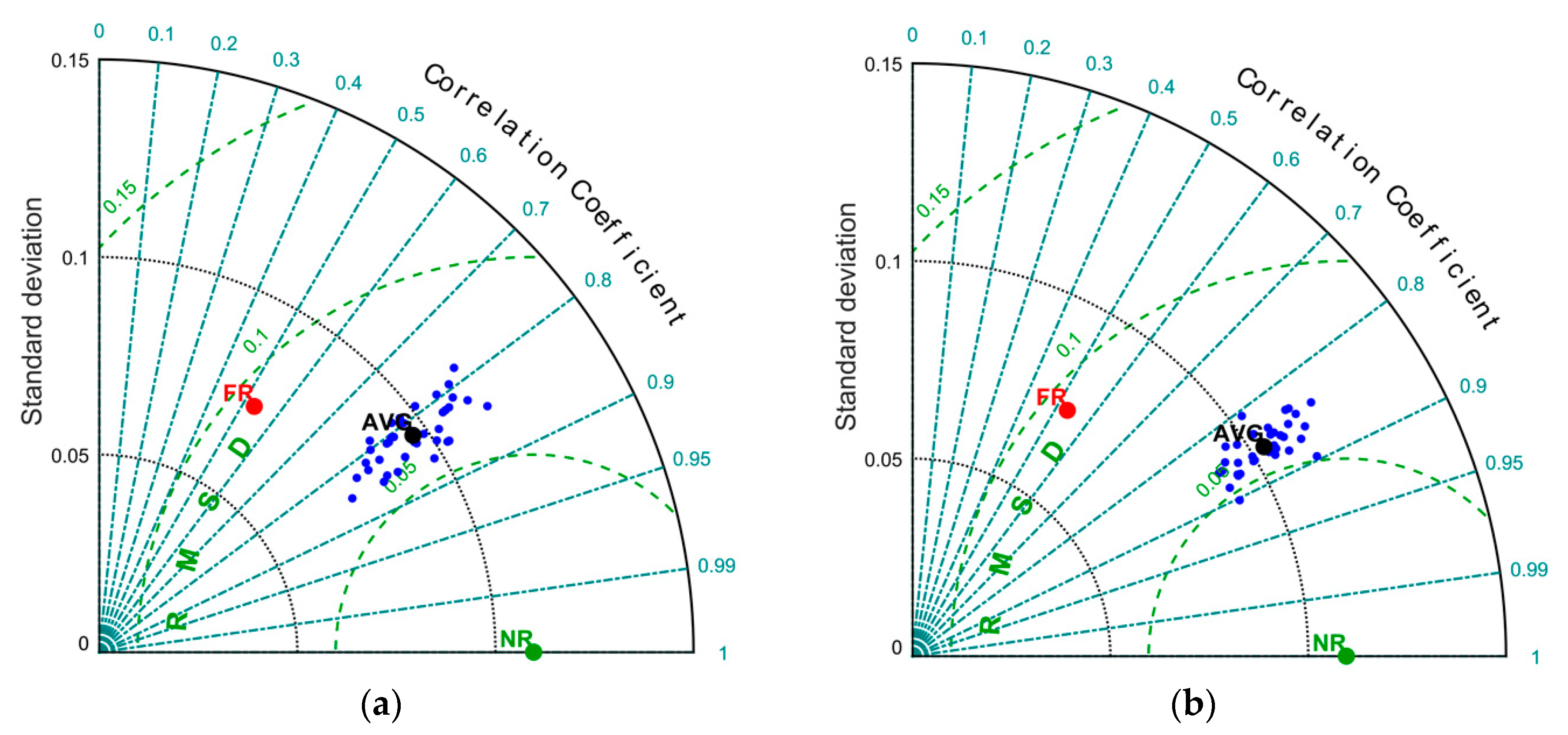
To compare each test, we adopt the Taylor diagram representation [36], which is often used in the operational field and allows collecting the same graph three of the most used statistical indices: the correlation, the centered root-mean-square error, and the standard deviations between two series (considering the Nature Run as the target). As in this study, we compare the maps of values at the same time, and correlation must be understood as a spatial correlation. These statistics are computed on the surface velocity components at the final time of the assimilation window, which is the initial condition for the five-day forecast run.

In the first experiment, we test the assimilation of an increasing number of velocity profiles, randomly located using the criteria described in the previous section. We start with 20 observation instruments (i.e., velocity profilers or ADCPs). As randomness can produce datasets more or less impactful for DA, the test is repeated considering different positions.

For the five-day assimilation window, two points are highlighted in Figure 5:

1.

The Nature Run (NR), that we assume as the true state of the system;

2.

The Free Run (FR), starting from the climatological state, which is poorly correlated with the NR (around 50%).

We find an excellent capability of the DA algorithm (ROMS-IS4DVar) to adjust the initial condition and bring the evolution of the state of the system closer to the truth.

Figure 5 shows a wide spread between the analyses produced by assimilating different datasets, each corresponding to a different network configuration. We observe a significant spread of the results around such average, as analysis data can have a stronger (around 0.8 for Dataset M) or weaker correlation (around 0.6 for Dataset U). Some analyses although characterized by a high correlation to the NR have lower standard deviations than the NR, hence they poorly represent the true circulation structures.

As an example, in Figure 6, we report the snapshots of the circulation of both the worst and the best analysis obtained, respectively, from the synthetic datasets corresponding to the configuration networks “M” and “U.”

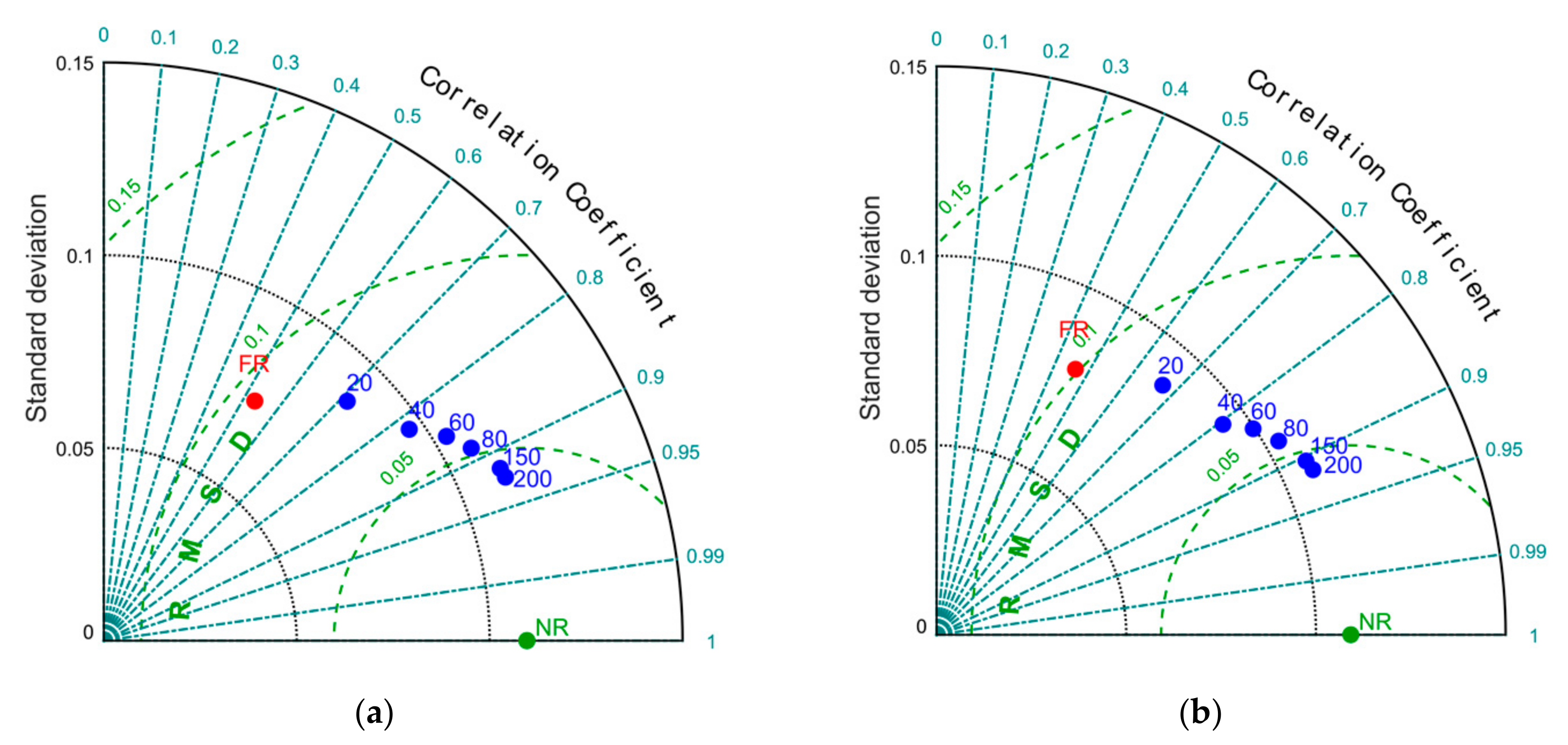
This first set of experiments is extended through the assimilation of a growing number of randomly positioned ADCPs (40, 60, 80, 100, 150, and 200).

Looking at the averaged statistics of analyses (named AVG in Figure 7), we have a positive effect of DA in improving the estimation of the model state as the number of observation points increases. At the same time, the statistical indices within each ensemble are increasingly closer to each other.

The results of all tests with the same number of observation points are summarized by means of a number of average points, each representing the averaged statistics of the related ensemble in Figure 8. We observe a progressively better quality of analyses in terms of all statistical indices (correlation, RMSE, and standard deviation) and a progressively lower benefit in the assimilation of additional observations. Indeed, as the number of observations increases, the marginal improvement of the analyses decreases. Therefore, a suitable strategy to localize measuring tools is especially impactful in observation networks characterized by a few instruments, which is the case of most in situ observation networks used in operational oceanography.

Figure 9 shows the improvement of the quality of analysis and forecast for an increasing number of observations. Forecast reliability, in terms of correlation and error, is strictly dependent on the quality of initial conditions; therefore, it is quite proportioned to the analysis.

By considering individually each analysis, some overlapping areas between the statistical scores of different ensembles are also shown in Figure 7 and Figure 9. This means that, in some cases, a significantly different number of assimilated data can approximately lead to the same improvement. Therefore, a relatively small number of well-positioned instruments can produce an analysis almost equivalent to that produced by a network of poorly located instruments, albeit larger. In fact, some analyses obtained with only 20 ADCPs have produced results equivalent to networks with 40 or even 60 ADCPs (Figure 7 and Figure 9).

In the second set of experiments, the positions of in situ observation instruments are identified by two elements: (1) the highest values of the projection on the velocity components of the dominant singular vectors, and (2) a fixed minimum distance among the instruments. As we mentioned in Section 2.2, the need to impose a minimum distance among instruments arises from the typical structure of the dominant singular vectors concentrated in relatively small areas.

In some experiments, not reported in this paper, we sample our DG system by extracting most measurements in the area of highly dominant SVs, but the results are even worse than those obtained with randomly positioned observations.

Distances are provided in dimensionless units, as they are divided by the barotropic Rossby deformation radius LR = (gh)1/2/f ≈ 900 km. We repeat the ensemble for testing different minimum distances from 0.04xLR to 0.28xLR.

Following the present observation strategy, the first observation point is located where the projection of the dominant SV on the velocity is maximum, and the following observation points lie farther than the chosen minimum distance.

The results of this set of experiments are shown in Figure 10 and Figure 11, in which we compare the analyses obtained in the first assimilation window (Figure 10) and, on average, for all the assimilation windows (Figure 11).

Looking at the first assimilation window (0−5 days), the worse dataset corresponds to an imposed minimum distance of the order of the spatial resolution, which is 0.04xLR. By increasing this minimum distance, we progressively obtained better correlation up to a value approaching 0.8, in turn corresponding to a minimum separation of about 0.25xLR. The observation positions of both the worst and the best dataset are reported in Figure 12. Considering other assimilation windows, the results are quite similar: the worst correlations are usually obtained for short minimum distances, and the correlation tends to increase when we separate the observation positions. The maximum correlation is found in the range of 0.15−0.25xLR (Figure 13).

Taking the average of all curves referred to the whole set of assimilation windows, the best correlations are obtained by imposing a minimum distance of about 0.2 xLR (Figure 13).

Datasets selected by imposing a distance up to 0.08−0.1 xLR produce worse analyses than randomly selected observations; the same occurs with minimum distances larger than 0.3 xLR. Conversely, in the range between 0.1 xLR and 0.25−0.3 xLR, this selection procedure produces, on average, analyses more reliable than that corresponding to random positioning.

Finally, as a third set of experiments, we test a procedure, still based on SVD, in which we impose a maximum correlation between the time series of the observed variables at the observation positions, instead of a fixed minimum distance. Such a limitation on the correlation between the time series of model velocities at observation points is introduced by imposing a minimum distance variable over the domain, and it is computed as explained in Section 2.2.

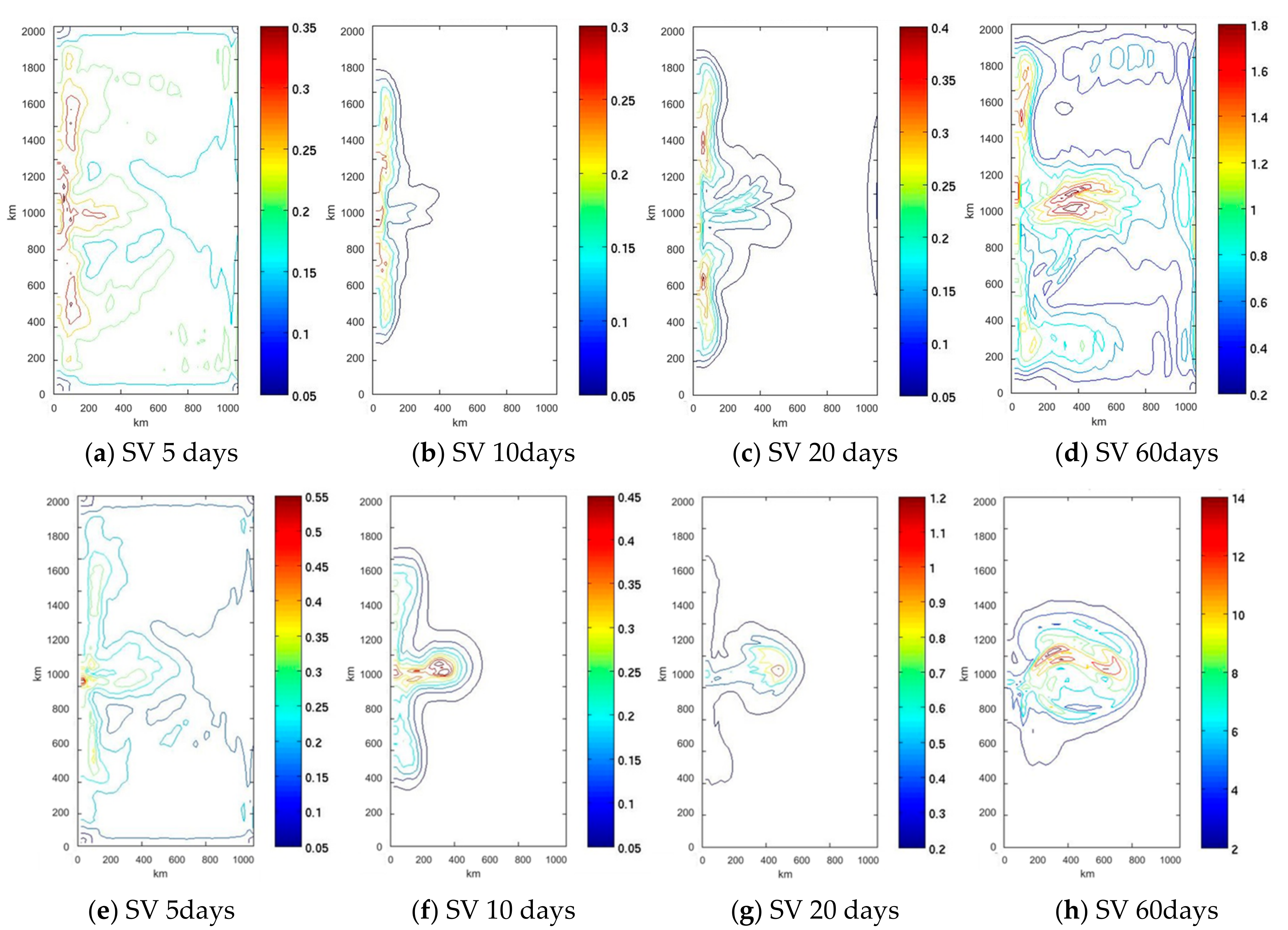
The selection procedure for this set of experiments is based on the map in Figure 4. Starting from the observation point in which we compute the maximum value of the projection of the SV onto the velocity, we identify the minimum distance to place additional observations through such a map derived from the correlation analysis.

It is important to underline that, in this procedure, the position of observation points are uniquely determined once a correlation threshold is defined. Such a threshold should be itself a calibration parameter of the sampling strategy to be selected on the basis of the correlation value that may guarantee the best comparison between analysis and the (virtual) truth. Although the correlation threshold is not calibrated in this study, such a unique configuration of the observation points is found to be the one that gives rise, on average, to the best analysis.

The average value of such a variable correlation distance is around 300 km, which is about 0.3xLR, slightly outside the “best” minimum distance found for the second set of experiments in which a fixed separation among observations is set. However, this distance, on the map in Figure 4, varies between lower values (around 150−200 km), near the convergence area, and higher values (>600 km) near the northern, southern, and eastern edges. The highest SVs are located within the area of lower correlation distances that fall within the range of 0.15−0.20 LR that we find, empirically, as an optimal distance interval using the fixed distance criterion.

The third procedure is able, on average, to improve the quality of the analysis model with respect to both the random procedure, and to the SVD-based procedure with a fixed distance among observations.

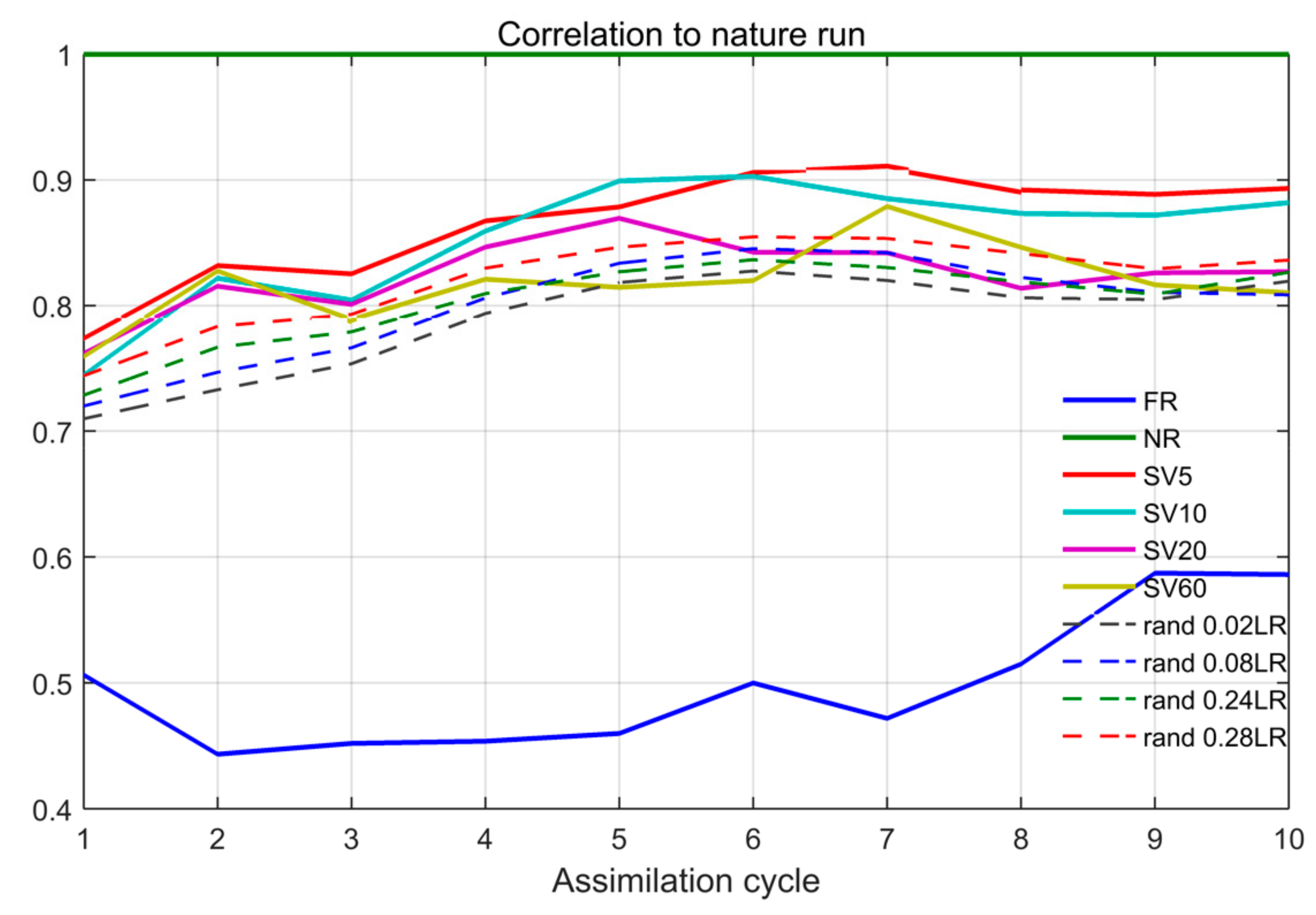
The observation strategy is tested for repeated assimilation cycles, as in the normal procedures adopted in the operational practice. A summary representation of results is shown in Figure 13. The observation strategy based on the combination of SVD and correlation analysis (solid lines) in most cases gives the best performances with respect to any random positioning procedure (dashed lines).

We also assess the sensitivity of the results to the optimization time for the SVD computation. In this case, the difference among the datasets, in terms of correlation with respect to the NR, is not so relevant, but we find that the configuration of observation points obtained by the SVD on a shorter optimization period (5−10 days) gives the best results. In particular, the analysis corresponding to the SVD with an optimization time of five days (SV5 in Figure 13) always yields significantly better analyses than any other tested strategy.

4. Discussion and Conclusions

The marginal improvement of the reliability of an ocean forecasting system can be obtained by a proper design of the ocean-observing component.

The Singular Value Decomposition was already used by various authors in the field of Geophysical Fluid Dynamics (mainly in the atmosphere) for several purposes, including the identification of possible adaptive observation strategies. However, the analysis of the potential of this method is still rather lacking to provide effective and functional indications for the design of in situ observation networks.

In this work, we evaluate some possible SVD-based strategies to determine an optimal set of in situ observation points in the case only a limited number of observation tools are available. This situation is common in reality, given the high cost of installing and managing in situ observation networks, especially in the oceanographic field.

We compare three observation strategies aimed at reducing the forecast uncertainty obtained through an idealized Double-Gyre ocean model, with repeated analysis and forecast cycles, using the variational assimilation scheme ROMS-IS4DVar.

We first proceed to evaluate the benefit linked to the assimilation of randomly positioned observations. The assimilation algorithm in use always produces a positive improvement in the estimation of the state of the system. The effectiveness of this improvement is not straightforward, as it depends in a complex way on the number of observation points and also on the location of these points in the model domain. This is especially evident in case only a limited number of observations is available.

Having a limited number of observation tools, and looking for the combination of positions that gives maximum benefit to DA, we assume that a fundamental indication for selecting observation points can be provided by the study of the areas in which the maximum error growth occurs. SVD is an excellent method for identifying these areas. The computation of the dominant Singular Vectors (SVs), and in particular of its projection on the physical components of interest, i.e., the velocity field, can give important information about error dynamics in the limit of validity of the linear tangent model. However, as the highest values of such SVs components can be concentrated in small areas, information obtained from points too close to each other is likely to be too correlated. To avoid this effect, we test two criteria:

• A first criterion, based on a rigid distance, is able to identify an optimal separation distance, which, in this case, is equal to about one-fifth of the Barotropic Rossby Deformation Radius. Around this value we have, on average, the best skills for the analysis model compared to the Nature Run assumed as truth;
• A second criterion, based on the maximum correlation between points, adopts a variable minimum distance among observation points. This criterion defines uniquely the position of observation points and provides better results both with respect to random simulations and with respect to the former optimization criterion.

Further improvements of the last criterion can be achieved through an accurate calibration of the threshold correlation parameter. However, even when adopting a threshold parameter of the first attempt, the obtained results are, on average, better than any formerly adopted strategy.

The extension of this method to real applications must take into account other factors, such as the presence of other variables of interest or a more accurate characterization of the observation error. In cases of ocean models more complex than the ocean DG, when baroclinic effects and density variations are more important, an SVD-based observation strategy should also evaluate the projection of the dominant SV on other variables, such as temperature and salinity, as any observation strategy cannot disregard the acquisition of density profiles. The application of this method to real ocean systems will also require a careful characterization of measurement errors, estimated from the performances of real observation instruments.

Testing such criteria to the design of observation networks, as in the standard Observing System Simulation Experiments (OSSEs) used for simulating the possible benefits of observing systems, could be of great interest. Indeed, most existing ocean observation networks are not designed from the very beginning using objective criteria to optimally support analysis/forecast models. Suitable design strategies are therefore needed for both making up new observation systems and expanding the capabilities of existing observation networks in order to improve their efficiency for data assimilation.

References

1. OECD. The Ocean. Economy in 2030; Organisation for Economic Co-Operation and Development (OECD): Paris, France, 2016. [Google Scholar] [CrossRef]
2. She, J.; Allen, I.; Buch, E.; Crise, A.; Johannessen, J.A.; Le Traon, P.-Y.; Lips, U.; Nolan, G.; Pinardi, N.; Reissmann, J.H.; et al. Developing European operational oceanography for Blue Growth, climate change adaptation and mitigation, and ecosystem-based management. Ocean. Sci. 2016, 12, 953–976. [Google Scholar] [CrossRef] [Green Version]
3. Tanhua, T.; McCurdy, A.; Fischer, A.; Appeltans, W.; Bax, N.J.; Currie, K.; Deyoung, B.; Dunn, D.C.; Heslop, E.E.; Glover, L.K.; et al. What we have learned from the framework for ocean observing: Evolution of the global ocean observing system. Front. Mar. Sci. 2019, 6. [Google Scholar] [CrossRef] [Green Version]
4. Oke, P.R.; Larnicol, G.; Jones, E.M.; Kourafalou, V.; Sperrevik, A.K.; Carse, F.; Tanajura, C.A.S.; Mourre, B.; Tonani, M.; Brassington, G.B.; et al. Assesing the impact of observations on ocean forecasts and reanalyses: Part 2, Regional applications. J. Oper. Oceanogr. 2015, 8, s63–s79. [Google Scholar] [CrossRef]
5. Moore, A.M.; Arango, H.G.; Broquet, G.; Powell, B.S.; Weaver, A.T.; Zavala-Garay, J. The Regional Ocean Modeling System (ROMS) 4-dimensional variational data assimilation systems: Part I-System overview and formulation. Prog. Oceanogr. 2011, 91, 34–49. [Google Scholar] [CrossRef]
6. Smith, K.D.; Moore, A.M.; Arango, H. Estimates of ocean forecast error covariance derived from Hessian Singular Vectors. Ocean. Model. 2015, 89, 104–121. [Google Scholar] [CrossRef]
7. Lorenz, E.N. A study of the predictability of a 28-variable atmospheric model. Tellus 1965, 17, 321–333. [Google Scholar] [CrossRef] [Green Version]
8. Kantz, H.; Schreiber, T. Nonlinear Time Series Analysis; Cambridge University Press: Cambridge, UK, 2004. [Google Scholar]
9. Toth, Z.; Kalnay, E. Ensemble Forecasting at NMC: The Generation of Perturbations; NMC: Washington, DC, USA, 1993; p. 20233. [Google Scholar]
10. Ehrendorfer, M.; Tribbia, J.J. Optimal prediction of forecast error covariances through singular vectors. J. Atmos. Sci. 1997, 54, 286–313. [Google Scholar] [CrossRef]
11. Corazza, M.; Kalnay, E.; Patil, D.J.; Yang, S.-C.; Morss, R.; Cai, M.; Szunyogh, I.; Hunt, B.R.; Yorke, J.A. Use of the breeding technique to estimate the structure of the analysis “errors of the day”. Nonlinear Process. Geophys. 2003, 10, 233–243. [Google Scholar] [CrossRef] [Green Version]
12. Palmer, T.N.; Zanna, L. Singular vectors, predictability and ensemble forecasting for weather and climate. J. Phys. A Math. Theor. 2013, 46, 254018. [Google Scholar] [CrossRef]
13. Hansen, J.A.; Smith, L.A. The role of operational contraints in selecting supplementary observations. J. Atmos. Sci. 2000, 57, 2859–2871. [Google Scholar] [CrossRef] [Green Version]
14. Farrell, B.F.; Ioannou, P.J. Generalized stability theory. Part I: Autonomous operators. J. Atmos. Sci. 1996, 53, 2025–2040. [Google Scholar] [CrossRef]
15. Farrell, B.F.; Ioannou, P.J. Generalized stability theory. Part II: Nonautonomous operators. J. Atmos. Sci. 1996, 53, 2041–2053. [Google Scholar] [CrossRef] [Green Version]
16. Wikle, C.K. Atmospheric modeling, data assimilation, and predictability. Technometrics 2005, 47, 521. [Google Scholar] [CrossRef]
17. Palmer, T.N.; Gelaro, R.; Barkmeijer, J.; Buizza, R. Singular vectors, metrics, and adaptive observations. J. Atmos. Sci. 1998, 55, 633–653. [Google Scholar] [CrossRef]
18. Buizza, R.; Montani, A. Targeting observations using singular vectors. J. Atmos. Sci. 1999, 56, 2965–2985. [Google Scholar] [CrossRef]
19. Langland, R.H.; Tóth, Z.; Gelaro, R.; Szunyogh, I.; Shapiro, M.A.; Majumdar, S.J.; Morss, R.E.; Rohaly, G.D.; Velden, C.; Bond, N.; et al. The North Pacific Experiment (NORPEX-98): Targeted observations for improved North American weather forecasts. Bull. Am. Meteorol. Soc. 1999, 80, 1363–1384. [Google Scholar] [CrossRef] [Green Version]
20. Buizza, R.; Cardinali, C.; Kelly, G.; Thépaut, J.-N. The value of observations. II: The value of observations located in singular-vector-based target areas. Q. J. R. Meteorol. Soc. 2007, 133, 1817–1832. [Google Scholar] [CrossRef]
21. Cardinali, C.; Buizza, R.; Kelly, G.; Shapiro, M.; Thépaut, J.-N. The value of observations. III: Influence of weather regimes on targeting. Q. J. R. Meteorol. Soc. 2007, 133, 1833–1842. [Google Scholar] [CrossRef]
22. Langland, R.H. Issues in targeted observing. Q. J. R. Meteorol. Soc. 2005, 131, 3409–3425. [Google Scholar] [CrossRef]
23. Bergot, T.; Hello, G.; Joly, A.; Malardel, S. Adaptive observations: A feasibility study. Mon. Weather. Rev. 1999, 127, 743–765. [Google Scholar] [CrossRef]
24. Gelaro, R.; Langland, R.H.; Rohaly, G.D.; Rosmond, T.E. As assessment of the singular-vector approach to targeted observing using the FASTEX dataset. Q. J. R. Meteorol. Soc. 1999, 125, 3299–3327. [Google Scholar] [CrossRef]
25. Langland, R.H.; Rohaly, G.D. Adjoint-Based Targeting of Observations for FASTEX Cyclones; Naval Research Lab: Monterey, CA, USA, 1996. [Google Scholar]
26. Pu, Z.X.; Kalnay, E. Targeting observations with the quasi-inverse linear and adjoint NCEP global models: Performance during FASTEX. Q. J. R. Meteorol. Soc. 1999, 125, 3329–3337. [Google Scholar] [CrossRef]
27. Bishop, C.H.; Toth, Z. Ensemble transformation and adaptive observations. J. Atmos. Sci. 1999, 56, 1748–1765. [Google Scholar] [CrossRef]
28. Szunyogh, I.; Toth, Z.; Emanuel, K.A.; Bishop, C.H.; Snyder, C.; Morss, R.E.; Woolen, J.; Marchok, T. Ensemble-based targeting experiments during fastex: The effect of dropsonde data from the lear jet. Q. J. R. Meteorol. Soc. 1999, 125, 3189–3217. [Google Scholar] [CrossRef]
29. Haidvogel, D.; Arango, H.; Budgell, W.; Cornuelle, B.; Curchitser, E.; Di Lorenzo, E.; Fennel, K.; Geyer, W.; Hermann, A.; Lanerolle, L.; et al. Ocean forecasting in terrain-following coordinates: Formulation and skill assessment of the Regional Ocean Modeling System. J. Comput. Phys. 2008, 227, 3595–3624. [Google Scholar] [CrossRef]
30. Speich, S.; Dijkstra, H.; Ghil, M. Successive bifurcations in a shallow-water model applied to the wind-driven ocean circulation. Nonlinear Process. Geophys. 1995, 2, 241–268. [Google Scholar] [CrossRef] [Green Version]
31. Moore, A.M.; Arango, H.G.; Di Lorenzo, E.; Cornuelle, B.; Miller, A.J.; Neilson, D.J. A comprehensive ocean prediction and analysis system based on the tangent linear and adjoint of a regional ocean model. Ocean. Model. 2004, 7, 227–258. [Google Scholar] [CrossRef]
32. Shen, J.; Medjo, T.; Wang, S. On a wind-driven, double-gyre, quasi-geostrophic ocean model: Numerical simulations and structural analysis. J. Comput. Phys. 1999, 155, 387–409. [Google Scholar] [CrossRef] [Green Version]
33. Kalnay, E. Atmospheric Modeling, Data Assimilation and Predictability; Cambridge University Press: Cambridge, UK, 2003. [Google Scholar]
34. Buehner, M.; Zadra, A. Impact of flow-dependent analysis-error covariance norms on extratropical singular vectors. Q. J. R. Meteorol. Soc. 2006, 132, 625–646. [Google Scholar] [CrossRef]
35. Golub, G.H.; Van Loan, C.F. Matrix Computations; Johns Hopkins University Press: Baltimore, MD, USA, 1989. [Google Scholar]
36. Taylor, K.E. Summarizing multiple aspects of model performance in a single diagram. J. Geophys. Res. Atmos. 2001, 106, 7183–7192. [Google Scholar] [CrossRef]
Figure 1. Surface current field (arrows) and Sea Surface Height (SSH) (m) of (a) the steady solution, (b) the climatological state, and (c) the initial state of the Nature Run for the first assimilation window.
Water 12 03445 g001
Figure 2. The 200 dominant singular values computed on an optimization time of 5 days (a) and an optimization time of 60 days (b).
Water 12 03445 g002
Figure 3. Sum of projections on the horizontal surface velocities of the 200 dominant initial singular vectors, for different optimization times (ad). Similar sum of projections computed for the first 200 final singular vectors (eh). Singular values are used to weight Singular Vectors (SVs).
Water 12 03445 g003
Figure 4. Map of the correlation distances (km) related to a correlation threshold of 0.6.
Water 12 03445 g004
Figure 5. Representation of the ensemble of the analyses obtained from the assimilation of different datasets of velocity fields from 20 observation points randomly positioned (blue points), the Free Run (red point), and the Nature Run (green point) in the first assimilation window. The orange circle indicates the M dataset, whereas the cyan circle indicates the U dataset, which Figure 6 refers to.
Water 12 03445 g005
Figure 6. Vector maps of the analysis from the configuration network “M” (a) and “U” (c) at the end of the assimilation window (see Figure 5). The observation positions, taken from the Nature Run (NR), are represented in (b) (Dataset “M”) and (d) Dataset “U”).
Water 12 03445 g006
Figure 7. Representation of the ensemble of the analyses obtained from datasets of velocity measurements from, respectively, 40 (a), 60 (b), 80 (c), and 150 (d) observation points randomly positioned (blue points), Free Run (red point), and Nature Run (green point) in the first assimilation window.
Water 12 03445 g007aWater 12 03445 g007b
Figure 8. Representation of the average point representing a different ensemble of (a) the analyses obtained from datasets of velocity measures characterized by a different number of observation points randomly positioned: 20, 40, 60, 80, 150, and 200; (b) the subsequent forecast.
Water 12 03445 g008
Figure 9. Correlation (a) and error (b) of the average point representing a different ensemble size (whose members are reported by single dots) of the analyses and the subsequent forecast obtained from datasets of velocity measures characterized by a different number of observation points randomly positioned: 20, 40, 60, 80, 150, and 200.
Water 12 03445 g009
Figure 10. Representation in the Taylor diagram (a) and correlation graph (b) of the analyses obtained for the first assimilation window. Each case corresponds to a network configuration defined by the highest SVs and the minimum fixed distance, expressed as a fraction of the Rossby deformation radius. The green point and the green line correspond to the case of a variable distance based on the correlation map.
Water 12 03445 g010
Figure 11. Taylor’s diagram (a) and correlation graph (b) of the average statistics of the analyses obtained for all assimilation windows. Each case corresponds to a network configuration defined by the highest SVs and the minimum fixed distance, expressed as a fraction of the Rossby deformation radius. The green point and the green line correspond to the case of a variable distance on the correlation map.
Water 12 03445 g011
Figure 12. Observation points of dataset selected by the Singular Value Decomposition (SVD)-based procedure imposing a minimum distance of 0.08 LR (a), 0.24*LR (b), and, finally, produced by the SV-based imposing the correlation distance of Figure 10 (c).
Water 12 03445 g012
Figure 13. Correlation of analyses run to the Nature Run for the 10 cycles of the 5-day-long-assimilation windows where the observation networks were based on the correlation map of Figure 4 and the SVD computed for different optimization times: 5 days, 10 days, 20 days, and 60 days. The dashed lines represent the results for the random strategy plus a fixed minimum distance. The analyses are compared to each other and to the Free Run (blue line).
Water 12 03445 g013
Publisher’s Note: MDPI stays neutral with regard to jurisdictional claims in published maps and institutional affiliations.