1. Introduction
The Naval Weapons Industrial Reserve Plant (NWIRP) occupies about 40 km
2 in southwest McGregor, Texas on a topographic divide underlain by a shallow groundwater system within fractured limestone bedrock (
Figure 1). The NWIRP began manufacturing explosives in 1980 [
1,
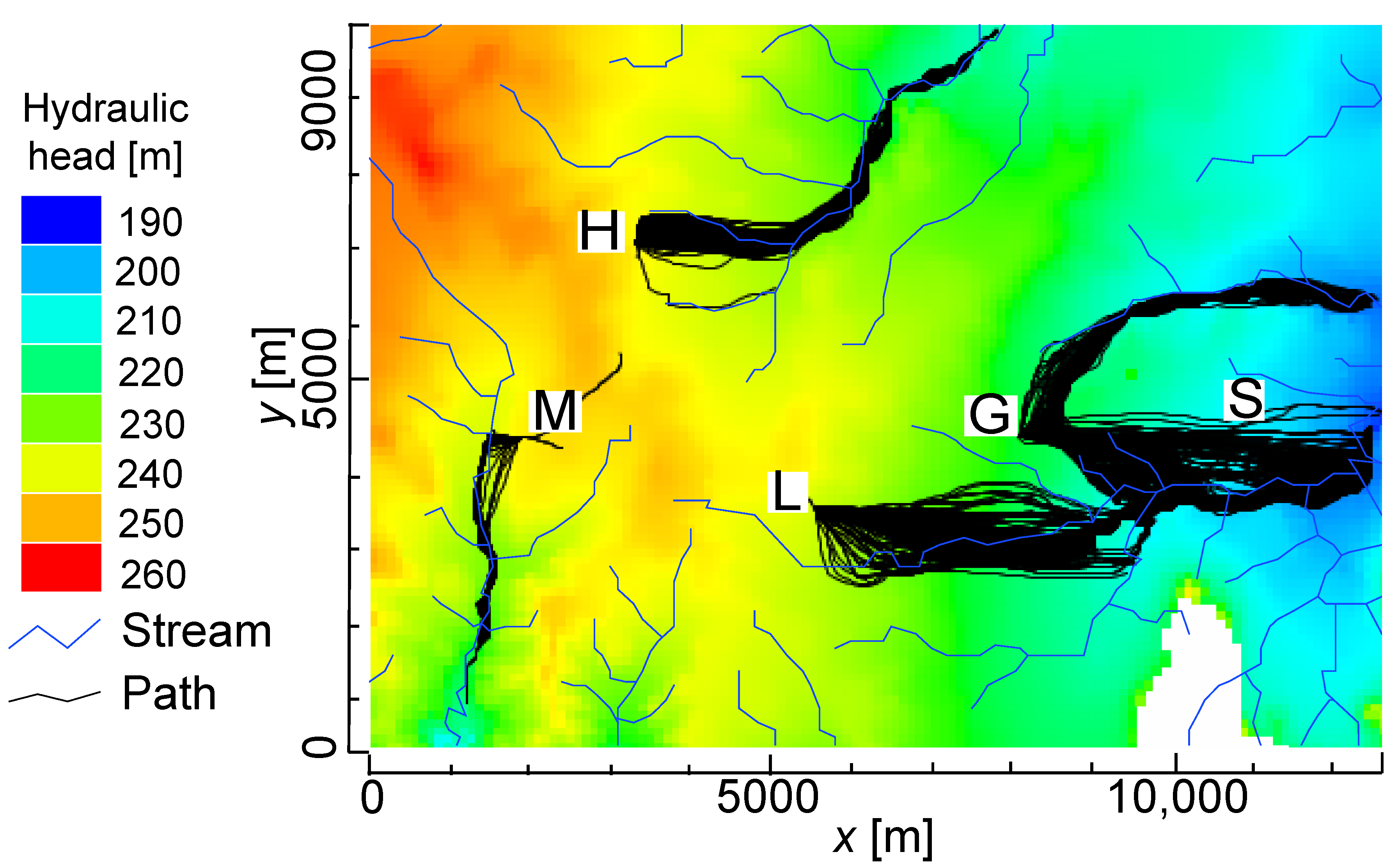
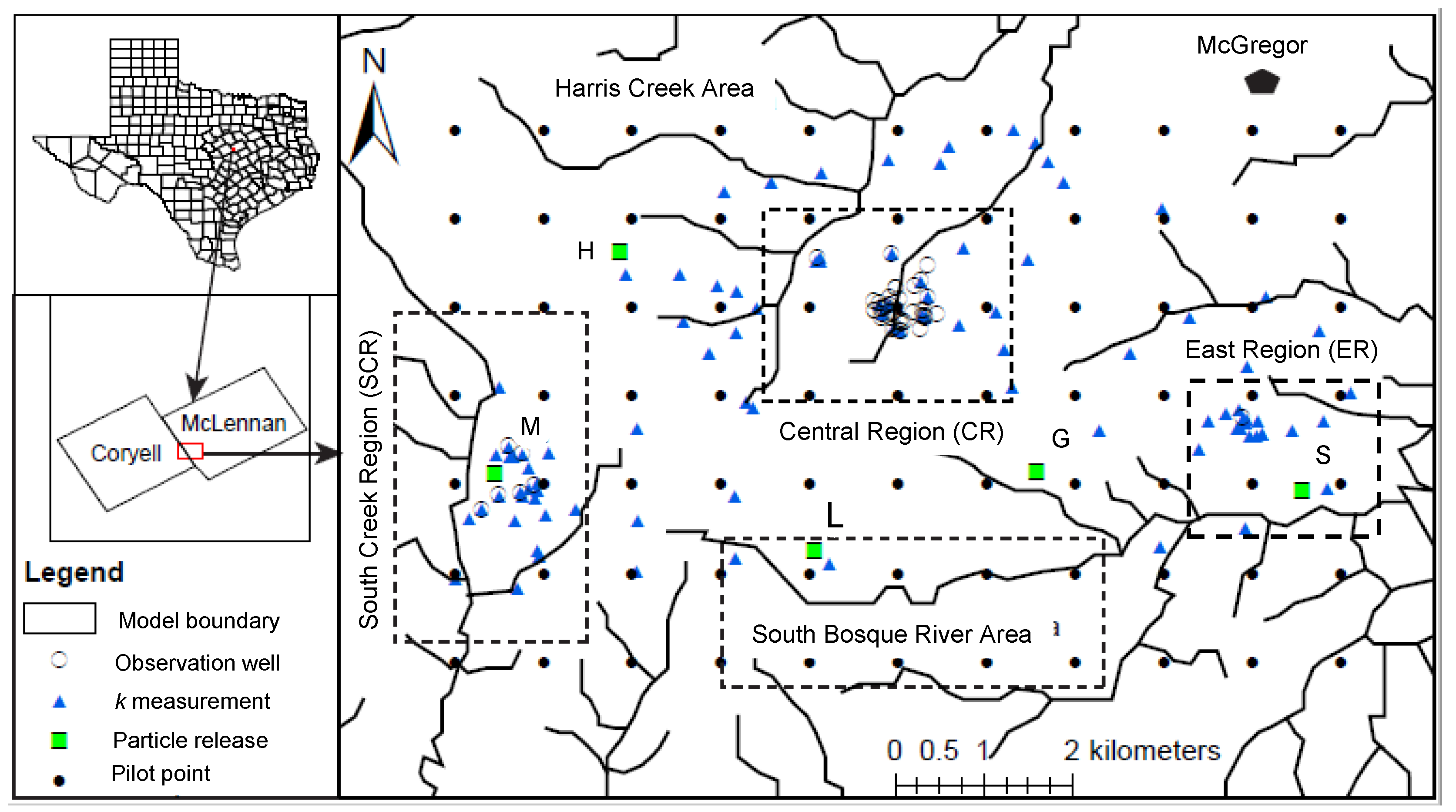
2] and stored several hazardous chemical wastes including ammonium perchlorate at five administrative locations: G, H, L, M, and S (see
Figure 1) those were found in lakes and streams surrounding the plant in 1998 [
3,
4]. Such short travel times were inconsistent with estimates from groundwater velocities that suggested the contamination should not have entered streams and migrated offsite for decades [
5]. Authorities failed on two fronts: (1) they significantly underestimated travel times for contaminants to reach nearby streams and (2) they failed to appropriately monitor the system after discovery of wastes exiting the site.
To address these issues, a heterogeneous MODFLOW-NWT [
6] model was developed to simulate flow and transport at the NWIRP site. The model included two fractured layers (the upper and lower layers), topography, streams, and heterogeneous hydraulic conductivities. In addition, a MODPATH [
7] particle-tracking model estimated conservative tracer transport paths and transport times. Predictions were conditioned through calibration against 43 measured hydraulic heads. Uncertainties in these predictions were quantified and the most important parameters and observations identified.
Moreover, the Null-space Monte Carlo (NSMC) [
8,
9,
10] nonlinear uncertainty analysis technique was used to generate probability distributions of calibrated parameters and commensurate particle travel-time predictions. Briefly, the NSMC technique uses subspace approaches like singular value decomposition [
11] to identify only those model parameters informed by the observation dataset [
12]. This facilitates inversion of over-parametrized models by only calibrating those variables about which the dataset has information while relegating the rest to their user-preferred initial guesses through Tikhonov regularization [
13].
Based on linear and nonlinear uncertainty analyses using MODFLOW and MODPATH models of the NWIRP site, we quantified the times for particles to reach nearby streams, which ultimately feed into nearby rivers and lakes. We also suggested locations for additional monitoring wells and a future data collection plan to better characterize and monitor the site to support improved waste-containment operations. These additional data were selected to ensure the greatest reductions in model-prediction uncertainty.
Background
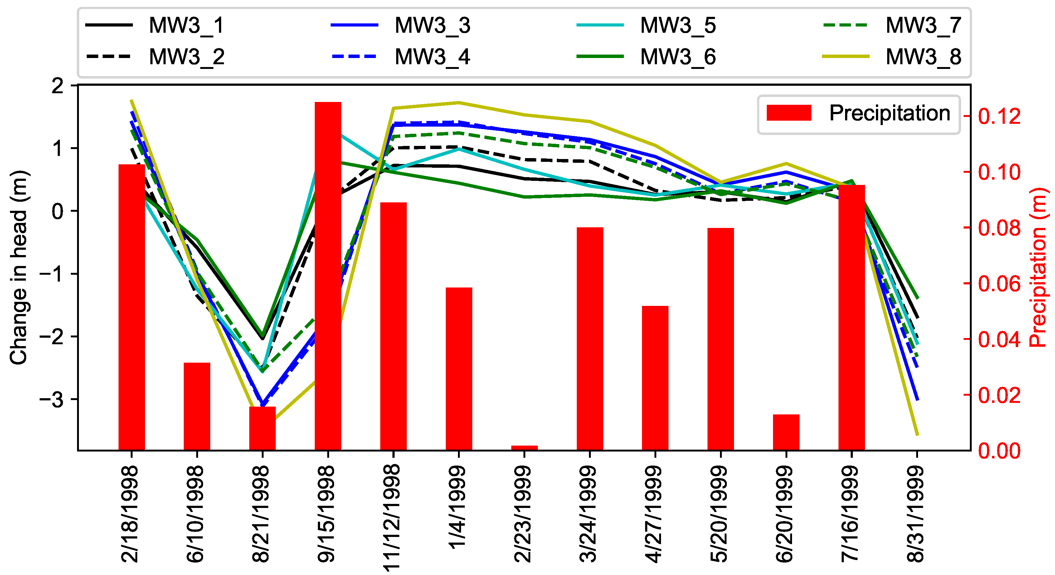
Ensafe Inc. [
3] estimated groundwater volumetric flux in Georgetown Limestone at 2 m/year using average gradients, hydraulic conductivity from slug-test data, and a total porosity while assuming homogeneous and steady groundwater velocities throughout the area. However, those estimates did not consider the increased fluxes and hydraulic heads affecting groundwater flow velocities during storm periods. The Georgetown Limestone, similar to other fractured carbonates like the Austin Chalk, exists as an upper, highly fractured and unsaturated zone overlying a low-permeability, moderately fractured zone [
14,
15,
16,
17,
18]. Recharge from precipitation significantly increases lateral flow through the Georgetown Limestone when the water table rises into the upper, highly fractured zone. The water table is sensitive to recharge (storms) as shown in
Figure 2. A rising water table can mobilize dissolved perchlorate such that it enters the upper zone where it is more easily transported off site. Even though some dissolved perchlorate is transported off site, the source persists as residual perchlorate in the lower fractured zone awaiting remobilization during the next storm (see
Figure 3).
2. Modeling Approach
The level of parametrization of an environmental model should be commensurate with the quality and quantity of data used in its calibration to ensure confidence in the range of predictive possibilities [
12,
20]. Calibration is constrained by the information content of the calibration data set (plus expert judgment) and linear predictive uncertainty can be assessed even before a calibration exercise. Parameter uncertainty along with observation worth can be quantified [
21,
22]. Post-calibration, the NSMC method facilitates a nonlinear assessment of parameter and prediction uncertainties [
22], but even with the use of super parameters (linear combinations of estimable parameters) to reduce the number of model calls, the approach can still be computationally intensive. The NSMC approach determines those parameters that are most informed by the calibration dataset and focuses on calibrating those parameters. For parameters that are not strongly informed by the calibration dataset, regularization techniques maintain those parameters close to their user-specified values.
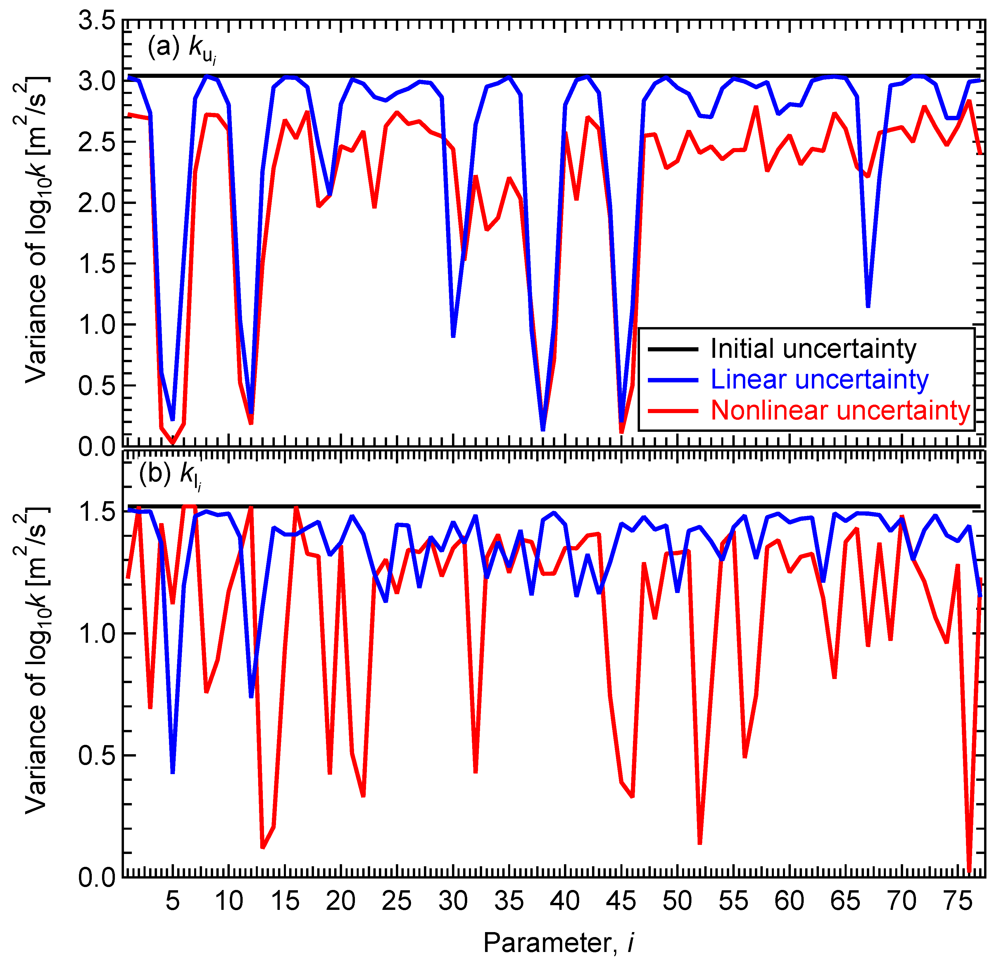
Predictive uncertainty analyses can be undertaken with a calibrated model using methods based on the propagation of variance [
22], which acknowledges that historic observation can be replicated with many non-unique parameter combinations. Predictive uncertainty reduction is calculated based on the pre- and post-calibration parameter uncertainties, where pre-calibration parameter variances (uncertainties) are specified according to measurements and expert judgment while post-calibration uncertainties are revealed through the calibration process and commensurate post-calibration analyses. Reductions in uncertainties in model predictions result from the information content in the calibration dataset through the decrease in pre-calibration parameter uncertainties upon calibration. Solution-space uncertainty, usually the smaller of the two, is due to uncertainty in the calibration data (i.e., measurement error). Null-space uncertainty is due to shortcomings in the data or model that preclude precise identification of the parameter (i.e., many parameter combinations can calibrate the model about equally well). The mathematical process of distinguishing solution- from null-space uncertainty is achieved through singular value decomposition (SVD), which is conducted with straightforward mathematical vector and matrix manipulations [
21,
22].
Measurement errors (observation noise) can never be eliminated and these impact predictive uncertainties. The calibration process minimizes the weighted-sum-of-squares differences, the objective function, between site observations and their corresponding model predictions. Both quantitative (observation noise, measurement accuracy, number of measurements comprising an observation, etc.) and qualitative (expert judgment) metrics should be used to specify weights in the objective function.
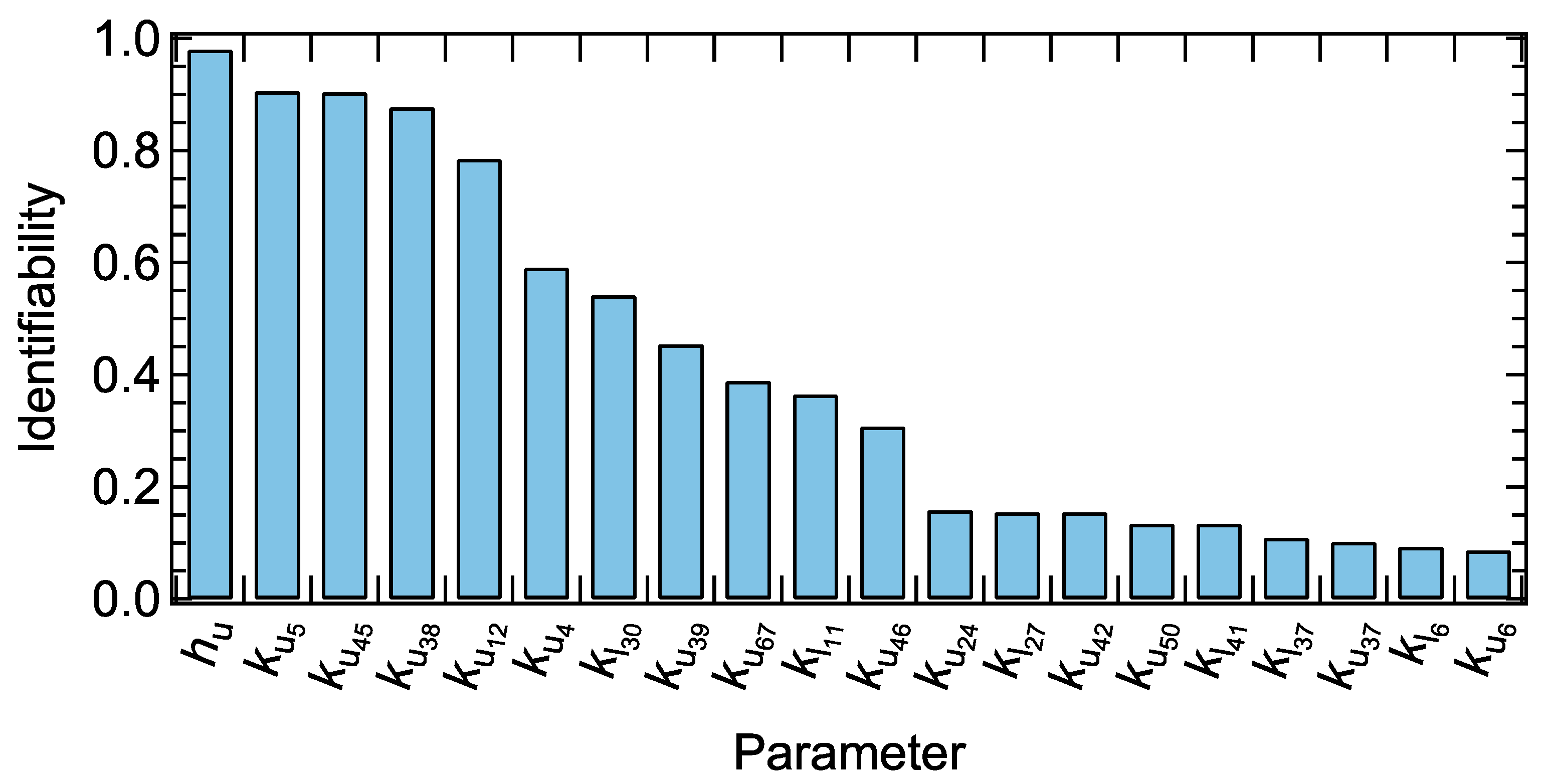
Identifiability is a metric indicating the calibration data’s ability to constrain a model parameter [
23]. Quantitatively, it is the direction cosine between a parameter and its projection onto solution-space uncertainty. Identifiability can be used in both model design and implementation to assess whether a model needs more calibration data to reduce parameter uncertainty while also quantifying the uncertainties in predictions that depend specifically upon that parameter.
Observation worth is quantified based on the reduction in uncertainty in a parameter or prediction that is accrued through the acquisition of that data point [
24]. Reduction in these uncertainties below their pre-calibration level is a measure of the worth of an observation (or observation group) with respect to that parameter or prediction.
The NSMC technique generates multiple, unique parameter fields that satisfy both the model-to-measurement misfit (i.e., a sufficiently low objective function) and parameter-reality constraints (i.e., parameters cannot be assigned unrealistic values) and it quantifies post-calibration parameter and prediction uncertainties [
25]. It generates a suite of equally likely and realistic parameter fields that are used to make predictions. Generating parameter fields involves three steps: (1) generating random parameter fields according to pre-calibration uncertainty, (2) perturbing pre-calibrated parameters by removing the solution-space uncertainty, and (3) a brief model calibration with three optimization iterations using fewer parameters or (super parameters), which are linear combinations of those parameters that have their pre-calibration uncertainty reduced by a significant amount (user defined, but for example >10%). Uncertainty in a prediction can thereby be assessed through construction of an empirical probability density function (PDF) assembled by running the model using each NSMC parameter field realization to generate PDFs of predictions.
The NSMC approach is faster than the related Markov Chain Monte Carlo (MCMC) approach, which is a Bayesian technique that samples parameters/predictions to obtain posterior PDFs [
22]. The MCMC approach requires two steps: Monte Carlo random sampling for all model parameters, not just those constrained by data, and Markov Chain sequencing of events that are probabilistically related. Essentially, MCMC methods approximate parameter posterior distributions by random sampling in a probabilistic space and then making the corresponding model runs. Similar to NSMC, a Bayesian analysis provides post-calibration parameter estimates with quantified probabilities. For models with long run times and many parameters, MCMC becomes computationally expensive while Doherty [
22] demonstrated that the additional model runs required by MCMC yield insignificant accuracy gains over NSMC.
2.1. Conceptual Model
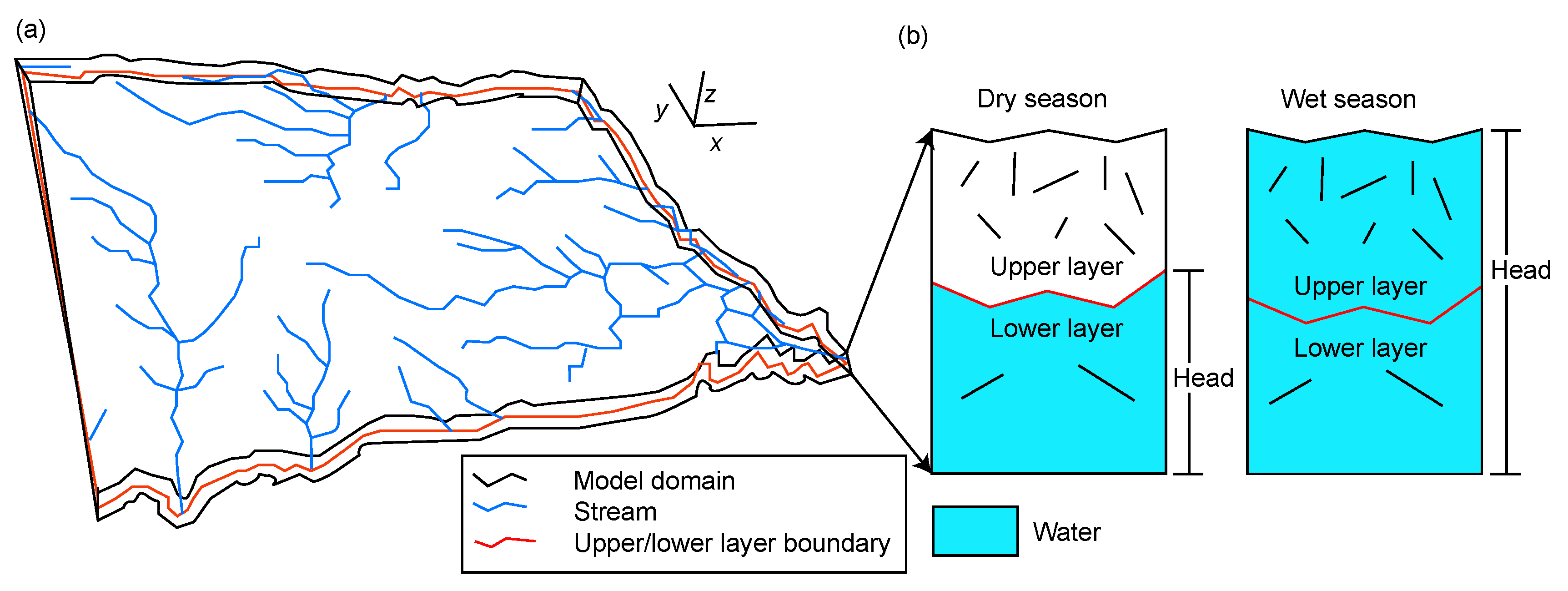
The conceptual model was built using four digital elevation maps (DEMs) from the Texas Natural Resources Information System website [
26] to create the model topography. GIS [
27] and SURFER [
28] were used to mosaic and grid the DEM data [
29]. The conceptual model also included local rivers, streams, creeks, and spring as shown in
Figure 3a. The model comprised two 4-m-thick layers representing the upper, weathered layer and the lower, less-permeable limestone. The NWIRP model domain and terrain-following layers were adjusted according to the topographic elevation (see
Figure 3a). The top of the upper model layer was assumed 2
below the land surface. The bottom of the model was established uniformly 10
below surface [
29]. Average precipitation from 1960 to 2015 was
. A base-flow study conducted in a nearby similar geologic setting indicated that 7% of total precipitation infiltrated to the aquifer [
29,
30], so recharge was assigned
. Due to lack of transient recharge and head data, a steady-state numerical model (see
Section 2.2) was developed assuming that the upper layer was fully saturated during the storm periods; this upper layer was, on average, five orders of magnitude more conductive than the bottom layer.
2.2. Numerical Model Development
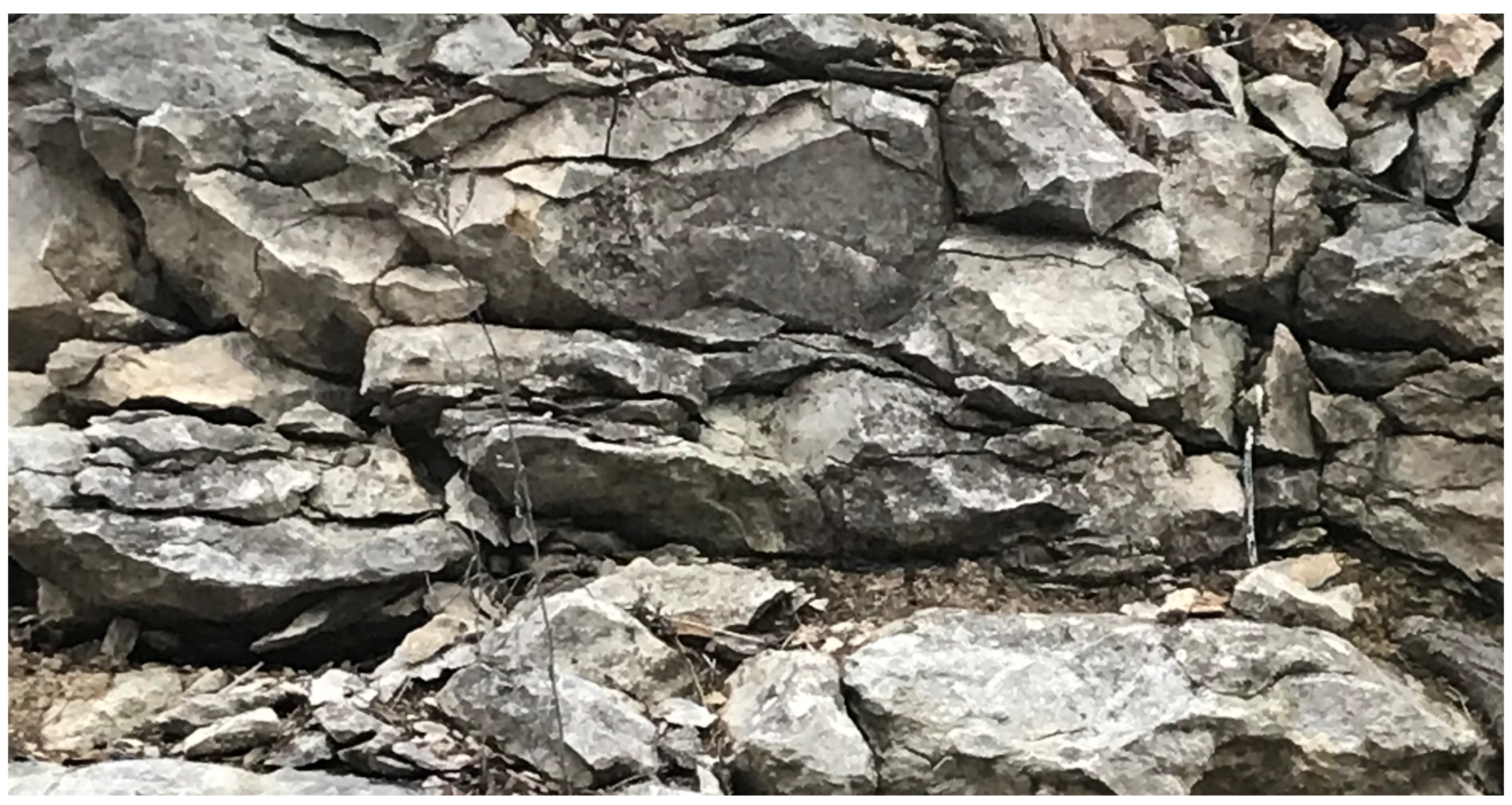
The upper layer in the model domain is densely fractured (
Figure 4); however, the fracture system has not been characterized for this site (e.g., no data on fracture length, spacing, aperture, orientation, etc.). A dense fracture system significantly enhances hydraulic conductivity of a rock formation. Sufficient data were available to characterize the system as an equivalent porous medium with enhanced hydraulic conductivity for the upper layer compared to the lower layer. Therefore, this effort started by developing groundwater and particle tracking models of the NWIRP site (
Figure 1), calibrating to available data, assessing observation worth, as well as quantifying uncertainties in parameters and particle travel-time predictions. Next, results from the NSMC approach were used to generate PDFs of pilot-point hydraulic conductivities and travel times. A grid-refinement study was performed to adopt an optimal grid resolution for this study. Cell dimensions along x and y axes for the grid-refinement study were
m
,
m
,
m
, and
m
, each with two layers.
Figure 5 shows that finer grids increased run times with negligible accuracy changes for piecewise homogeneous hydraulic conductivities. Therefore, we considered the model with two layers (representing the highly conductive upper layer overlying the less-conductive lower layer), 126 columns, and 97 rows with
cells.
Several boundary conditions (BCs) were applied in the model domain. Recharge through precipitation was specified at the top of the model while the lateral sides along with the bottom of the model were specified as no-flow boundaries. No-flow boundaries can affect results near the edges of the model, so the NWIRP regions of interest were always at least
km (15 cells) from the model edges. In addition to specified-flux and no-flow BCs, head-dependent-flux (HDF) BCs were assigned to cells containing a stream (drain cells in MODFLOW). In the HDF BC, a reference head and a conductance value were assigned at stream boundaries where water may only leave the flow system through the drain cell and it may not re-enter the groundwater system through cells further downstream. Also, if the hydraulic head in the stream cell fell below a certain threshold (e.g., bottom of the upper layer), the flux from the drain to the model cells was set to zero. The model was executed with MODFLOW-NWT [
6], which admits the drying and re-wetting nonlinearities of an unconfined aquifer [
6,
31]. Single particles were released at the midpoint of each layer from the five administrative areas and tracked until they exited the model domain at streams. Streams were modeled as potential discharge cells.
2.3. Parameters
Groundwater flow is fundamentally governed by the distribution of hydraulic conductivities. In conventional calibration methods, property uniformity or pilot-point distributions are used as the basis for spatial parameter distribution [
32]. In the absence of data, piecewise-homogeneous zones are often specified. If geologic zones are not piecewise-uniform, pilot points are distributed throughout such zones. Pilot-point property values were estimated during this calibration exercise and the hydraulic conductivities at model cells were assigned according to a kriging algorithm [
32]. Pilot points facilitate a smooth but plausible distribution of hydraulic properties over a geologic unit, which cannot be achieved using piecewise-uniform methods. The upper model layer had only a single hydraulic conductivity measurement, but one parameter over such a large region would lend false confidence in the solution because it would yield unrealistic homogeneity [
33]. Instead, a total of 77 pilot points (
Figure 1) were used in each layer such that hydraulic conductivity fields were developed with heterogeneity commensurate with the information available in the observation data set. The initial value of the horizontal hydraulic conductivity in the upper layer,
, was
for all 77 pilot points with a 1.5% porosity [
29].
Ensafe Inc. [
3] conducted 99 slug tests estimating horizontal hydraulic conductivities in the lower layer,
, ranging from
to
with mean
. These hydraulic-conductivity estimates were used in an exponential variogram with specified range and sill (variance) [
34]. The range and variance of log of hydraulic-conductivity measurements were 700
and 1.52, respectively, and using the 99 measured hydraulic conductivities, they were kriged (interpolated) onto each model cell. The vertical anisotropies and porosity of the lower layer were specified as one tenth of horizontal hydraulic conductivities and 0.5% [
29], respectively. Note, although it could facilitate a higher level of heterogeneity, no nugget effect was considered in this study because the empirical semi-variogram did not require it. Nevertheless, our broad hydraulic conductivity constraints during model calibration effectively interrogated a broad uncertainty range and admitted a high degree of heterogeneity.
The calculated range and sill were used to generate kriging factors for pilot points in the lower layer. Later, these factors were used to interpolate k onto the model grid using kriging. Because of exposure to weathering and erosional process, the upper layer is more heterogeneous even though it comprises similar rock types, so a larger variance was appropriate. Thus, a variance of 3.04 (almost twice that of the lower layer) was assigned to the upper layer with the same 700-m range as the lower layer. Variances of horizontal anisotropies for the upper and lower layers were set to 0.61. Parameter uncertainties and observation worth were calculated based on propagation of variance. Initially, a pre-calibration covariance matrix was calculated for the pilot points. The diagonal elements of the covariance matrix were the k variances while off-diagonal elements were non-zero covariances based on the 99 estimated hydraulic conductivities and their geospatial characteristics. This covariance matrix was used to generate pre-calibration pilot point realizations.
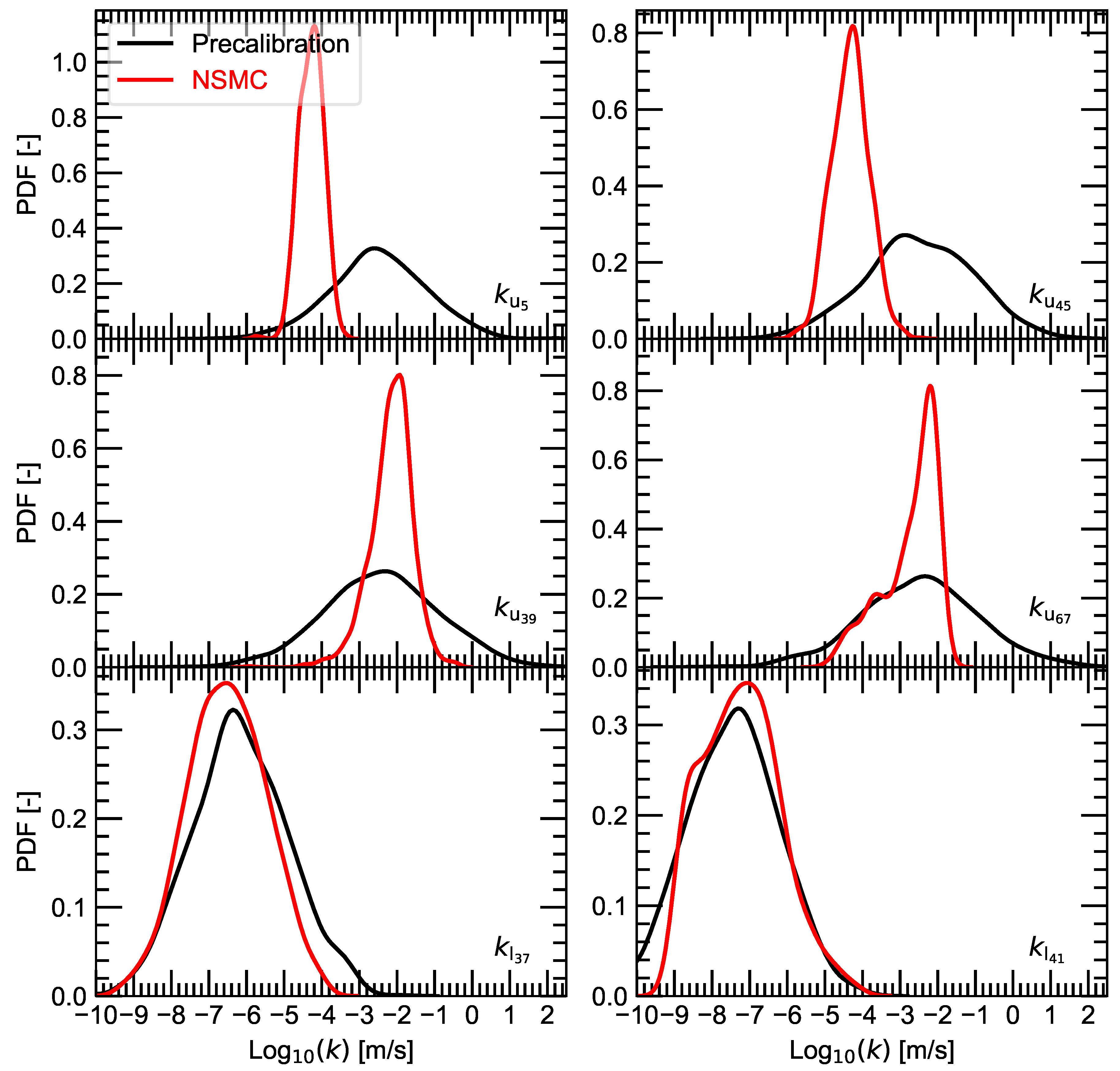
A total of 158 log-transformed parameters were adjusted during calibration. Parameters were subdivided into four groups: (1) 77 pilot-point-based horizontal hydraulic conductivities for the upper (–), (2) and lower (–) layers, (3) horizontal anisotropies for the upper, , and lower, , layers, and (4) vertical anisotropies for the upper, , and lower, , layers. Each hydraulic conductivity was assigned a pre-calibration lognormal probability distribution with mean of and for the upper and lower layers, respectively.
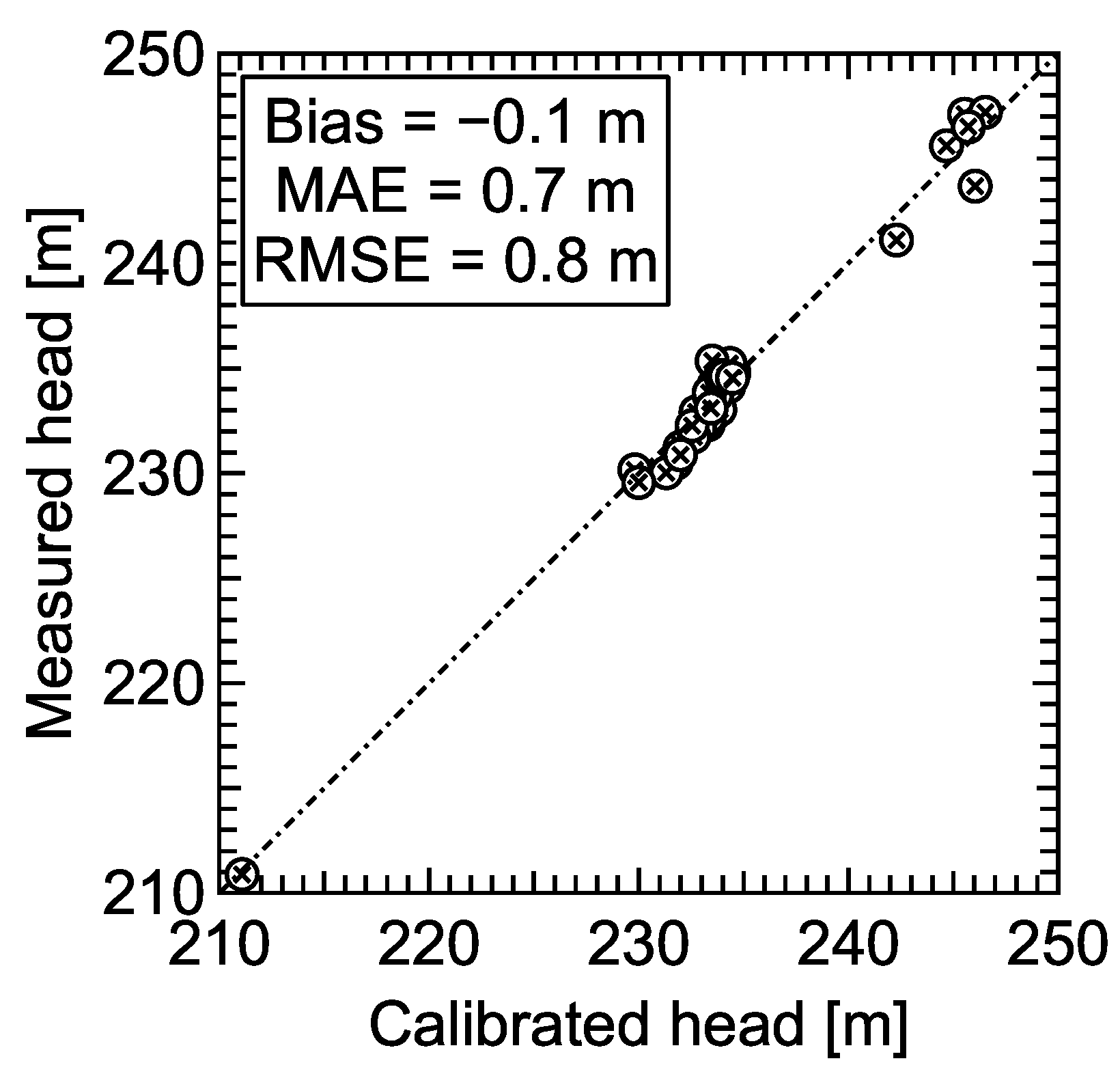
2.4. Calibration Data and Predictions of Interest
Because of model complexity and under-determinacy, regularization was used during calibration [
22] to reduce bias and to decrease the required number of model calls. The calibration was performed against 43 steady-state hydraulic heads (average hydraulic head if multiple measurements were available) at the monitoring wells indicated with open circles in
Figure 1 (see,
Appendix A for hydraulic-head data). Each observation was assumed equally important (equal weight). Predictions of interest were travel times for 10 particles released at the midpoints of the upper and lower layers at the five administrative hazardous storage sites labeled in
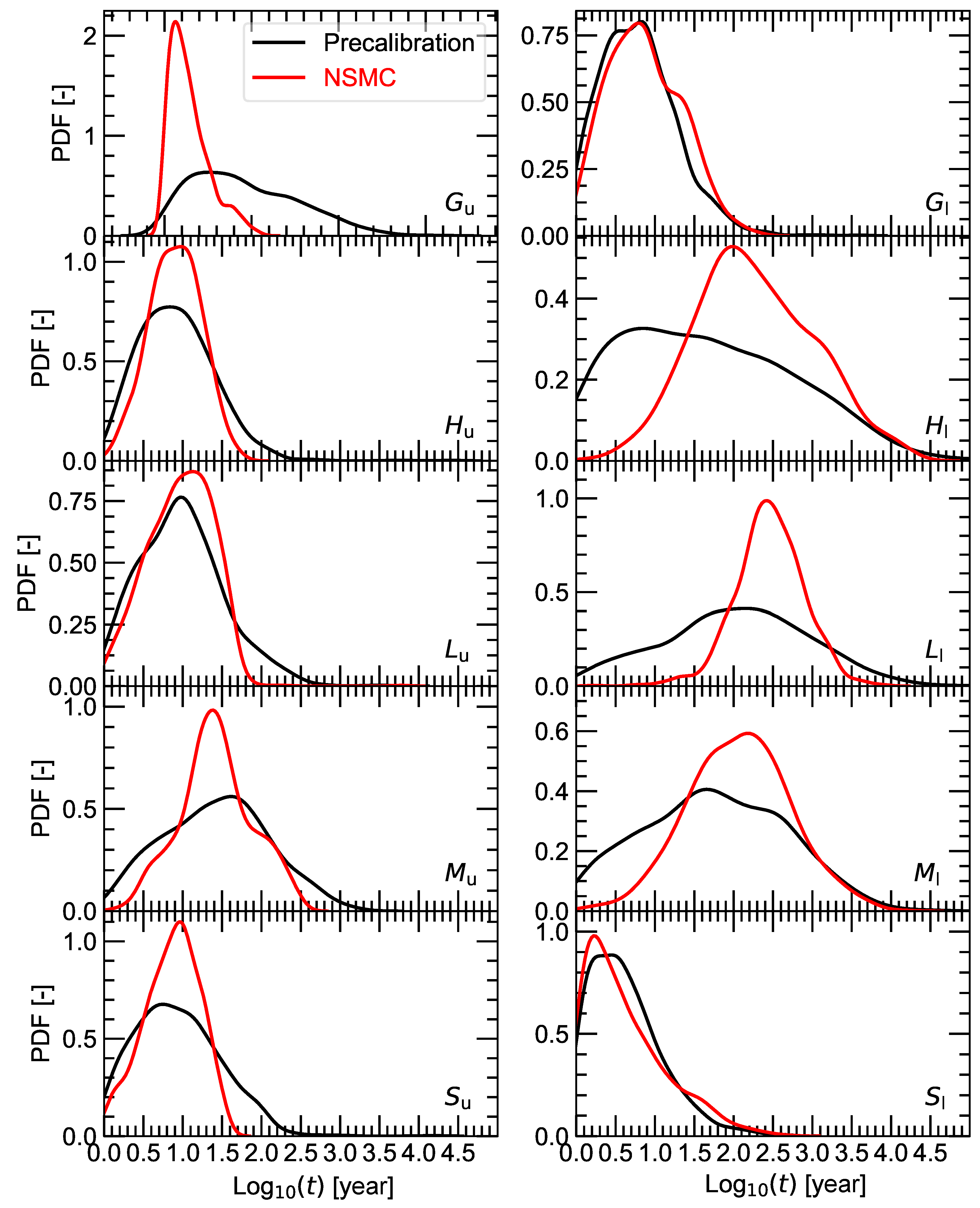
Figure 1 [
2]. Travel times for the particles were simulated and their uncertainties were quantified.
2.5. Calibration and NSMC
Steps in the calibration and uncertainty analyses included: (1) parametrization and calibration of the NWIRP groundwater model; (2) observation worth were calculated; (3) the effects of additional monitoring wells on travel-time predictions and observation worth were estimated; (4) uncertainties in travel-time predictions were then explored upon consideration of the new hypothetical observations (i.e., future borehole locations); and (5) post-calibration uncertainties of pilot points and particle travel times were assessed using the NSMC technique.
With 158 adjustable parameters (154 pilot points, two horizontal anisotropies, and two vertical anisotropies) and only 43 observations, this made this an ill-posed problem; not all parameters could be uniquely estimated [
11,
35]. Using SVD, it was determined that 25 unique linear combinations of parameters (super parameters) could be reasonably identified. In other words, all parameters (113 more than could possibly be identified by the 43 data points) were presented to the calibration and PEST’s subspace-regularization capabilities determine which parameters can be uniquely identified by the dataset and subsequently only focuses on those. Here, the dataset informed 25 parameters, which can be specified as linear combinations if there are strong correlations between some of them. For over-parametrized models, an NSMC analysis affords a more accurate, nonlinear assessment of predictive uncertainty. The NSMC approach was executed in three steps. First, a total of 1000 pilot-point realizations were generated (the mean of each pilot point stabilized by 1000 realizations) using a lognormal distribution with mean (from pump tests) and the pre-calibration covariance matrix. Second, each pre-calibrated parameter realization was perturbed by adding null-space uncertainty. This step calculated the orthogonal differences between calibrated parameters and random parameter realizations. Then, these differences were added to each realization of calibrated parameters to generate 1000 realizations of calibrated parameters with perturbations in the null space. For each of these null-space-projected parameter-field realizations, three iterations of a parameter calibration were undertaken perturbing pre-calibrated parameters by removing the solution-space uncertainty. Model results (hydraulic heads and particle travel times) using the newly generated parameter fields were necessarily similar to the results from the calibrated model; however, up to three calibration iterations (each yielding an updated Jacobian matrix and set of calibrated parameters) were undertaken to see if these steps could bring the model back into calibration. If a sufficiently low objective function could not be achieved after these three calibration iterations, then that parameter field was discarded (as not effectively calibrating the model or maintaining parameter reality).
4. Conclusions
Based on groundwater and particle-tracking simulations of the NWIRP site, calibration and model interrogation quantified parameter and predictive uncertainties, parameter identifiabilities, and observation worth for both existing and hypothetical monitoring wells. Using a linear analysis, pre-calibration parameter uncertainties were reduced up to 92% and 36 of 158 parameters exceeded a 10% reduction when constrained by the calibration data set. An identifiability study revealed that seven parameters were highly identifiable (>0.5) while 12 parameters had identifiabilities between 0.1 and 0.5. Travel-time uncertainties were reduced up to 92%. Using a nonlinear analysis, pre-calibration travel-time uncertainties were reduced by >50% for two particles released at site M and between 5 and 40% for the remaining sites. Vertical anisotropy did not play a significant role because there was minimal vertical flow in the model and no well data suggesting a vertical gradient.
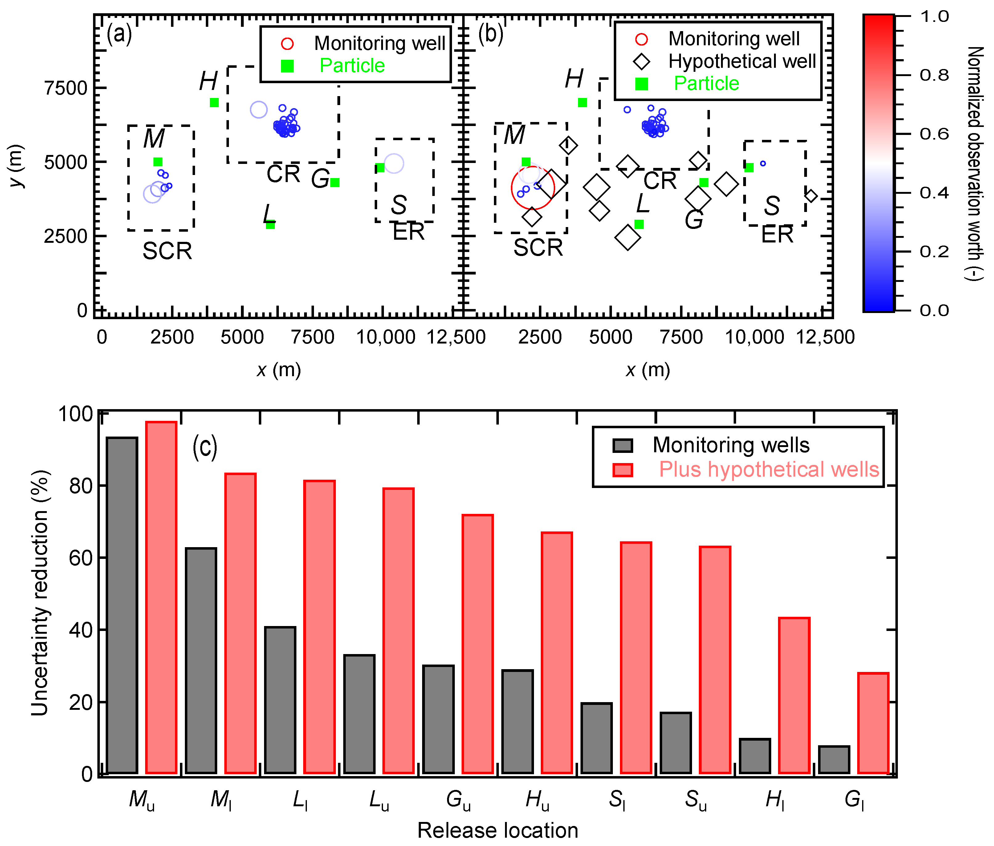
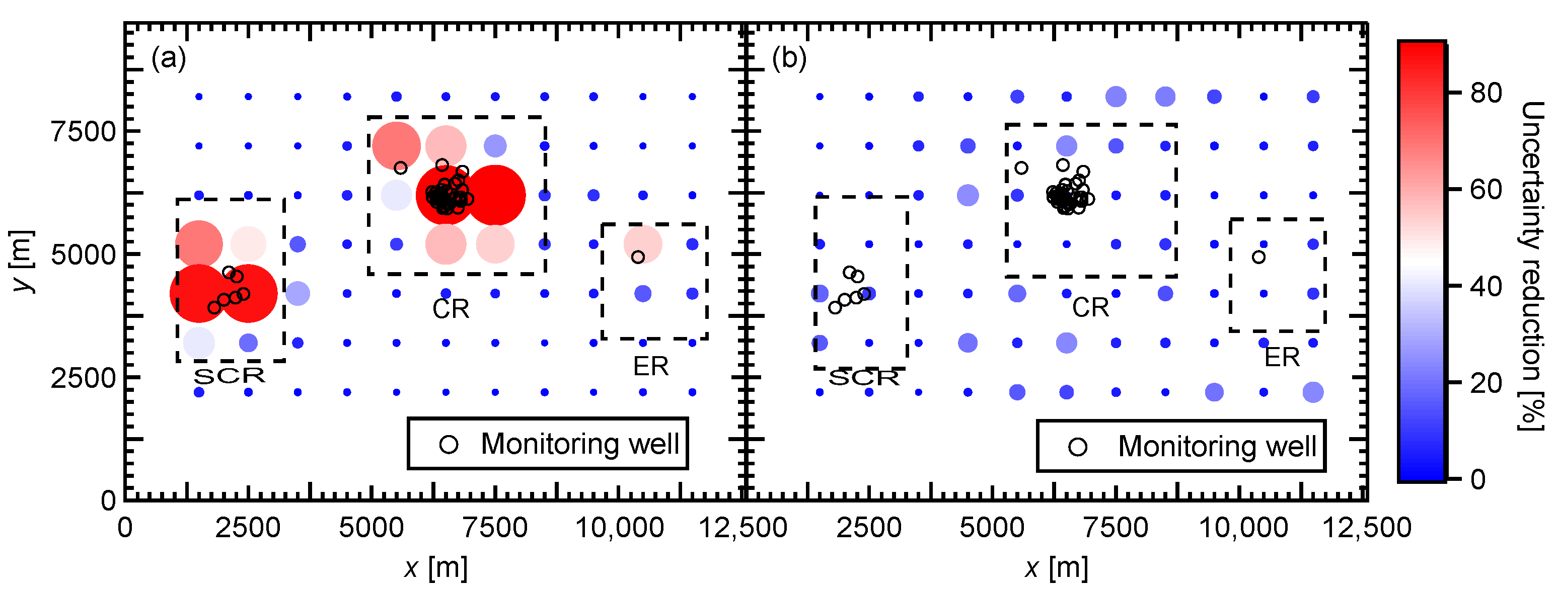
Also, this study generated pre- and post-calibration parameter distributions along with corresponding travel-time PDFs. The decreases in width of these distributions (variances) reflected the information content in the calibration data set. This study also predicted travel times for conservative particles to reach nearby streams and, for the upper layer, they exited the flow system within a year. An observation-worth analysis showed that the existing monitoring well network does not strongly constrain travel times. Suggested data collection, especially at the locations shown in
Figure 9b, could reduce travel-time for all particles by factors from 1.04 to 4.3. Ultimately, it is up to the regulator to determine how many wells must be added to reduce modeling uncertainties to a point where they are comfortable making remediation decisions based on simulated site behavior.
Any seriously contaminated site like NWIRP should undergo a rapid and detailed modeling study before further data collection and, of course, before making remediation decisions. For example, the authority collected clustered water-level measurements, which could have been optimized if a comprehensive study was conducted before drilling wells. In addition, no base-flow data were collected even though a single base-flow measurement significantly improves uncertainty quantification [
36]. This study also demonstrated that if a contaminant reached the upper layer (for example during storm events that raise the water table), it will travel much faster to surrounding streams. The predictive-uncertainty and observation-worth analyses determined the most important parameters and observations contributing to the greatest decreases in predicted travel-time uncertainties. Ultimately, the 43 poorly distributed water-level measurements over such a large model domain and the absence of base-flow data were notable shortcomings. This analysis can support decision making by identifying where additional wells should be located to achieve the greatest reductions in predictive uncertainty.
Looking to the future, transient modeling would be appropriate for this system, but it cannot currently be undertaken because of a lack of water-level time-series data. Although beyond the scope of this study, it would be reasonable to use these calibrated parameters in a transient model to assess other aspects of contaminant transport subject to storm or flood events. While a discrete fracture network model could be an alternative approach, the fractured system was not sufficiently characterized to support development of such a model. Also, chemical wastes were treated as conservative particles. Although a more complex transport model would also be of value, the necessary data (e.g., a comprehensive study on the chemical wastes including measurements of dispersion, matrix diffusion, sorption, decay, and other local or regional mixing phenomena for individual chemical constituents) are not available.


