Article

Setting Up of an Experimental Site for the Continuous Monitoring of Water Discharge, Suspended Sediment Transport and Groundwater Levels in a Mediterranean Basin. Results of One Year of Activity

by
Stefano Giorgio Pagano
1,2,†,
Donato Sollitto
2,†,
Marco Colucci
2,
Davide Prato
2,
Fabio Milillo
1,
Giovanni Francesco Ricci
1,* and
Francesco Gentile
1
1
Department of Agricultural and Environmental Sciences (Di.S.A.A.T), University of Bari, via Amendola 165/A, 70126 Bari, Italy
2
Basin Authority of the Southern Apennines District, Viale Lincoln-ex Saint Gobain’s Area, 81100 Caserta, Italy
*
Author to whom correspondence should be addressed.
Pagano and Sollitto contributed equally to this work.
Water 2020, 12(11), 3130; https://doi.org/10.3390/w12113130
Submission received: 9 September 2020 / Revised: 20 October 2020 / Accepted: 31 October 2020 / Published: 8 November 2020
(This article belongs to the Section Hydrology)

Abstract

:
The study of suspended sediment transport requires continuous measurement of water discharge to better understand the sediment dynamics. Furthermore, a groundwater monitoring network can support the stream discharge measures, as it reveals how the interactions between surface water and groundwater may affect runoff and consequently sediment transport during flood events. An experimental site for the continuous monitoring of water discharge, suspended sediment transport and groundwater levels was set up in the Carapellotto basin (27.17 km2), which is located in Apulia, Southern Italy. Seven flood events that occurred in the operation timespan were covered with a full record of both water discharge and sediment concentration. Some monitoring problems, largely due to the clogging of the float by mud, suggested to improve the experimental set up. The results show high values of suspended sediments concentration which indicate the sub-basin’s key role in the sediment delivery to the whole river system, while counter-clockwise hysteresis loops are the most frequent due to the basin characteristics. The effects of the interaction between surface water and groundwater are related not only to the flood magnitude but also to the hydrogeological features in the hyporheic zone.

1. Introduction

Suspended sediment dynamics in rivers involves erosion, transport, deposition and resuspension processes that occur within basins. The suspended sediment concentration (SSC) in streams may evolve over time, in response to the basin morphology, climate and human disturbances [1,2,3,4]. The study of suspended sediment transport at the basin scale is useful for the assessment of water quality associated with fluvial sediments [5], for restoration purposes [6], for estimating erosion processes, sediment production and the effectiveness of control measures [7,8,9].
SSC monitoring in a basin is usually based on water sampling in different locations to measure solid transport within the river network. The efficiency of monitoring depends on the number of sampling sites in the measurement network and on the sampling frequency. In most countries, especially in the Mediterranean areas, concentration and discharge data are very poor or non-existent, and in some, the number of samplings is decreasing [10,11].
Water discharge (Q) measurement is often carried out by coupling acoustic and optical systems [12,13]. The former emits a sound toward the water surface and measure the time it takes to get back. The latter measure the water velocity on the flow surface using the Doppler effect. Calibration against current meter data is needed, as well as an accurate survey of the cross-section.
Significant variations of the factors affecting SSC occur at the event scale. During flood events, the Q and SSC usually do not show a univocal relationship but describe hysteretic behaviors. The study of hysteresis patterns is a common technique to study the main factors in suspended transport processes [3,14,15,16,17,18], as well as to identify the sediment source areas [2,19,20,21,22]. Williams [23] classified the main types of hysteresis, defining a single line (no hysteresis), circular loop (with a clockwise or counter-clockwise direction), and eight-shaped loop.
Therefore, sediment transport studies require at the same time continuous monitoring of both Q and suspended sediment [24,25]. Turbidity measurement is currently used as a surrogate for SSC, and needs calibration against manual samples, mostly during floods [7,26,27,28,29,30,31].
In many basins, groundwater and surface water are hydraulically connected, and their interaction can take place in different ways based on the hydrogeological conditions and may have important effects on the river discharge [32]. The interaction between surface water and groundwater may also have important effects on the flood formation through the bank storage processes.
The assessment of groundwater and surface water connectivity is often complex because it depends on many factors, such as the distribution and the magnitude of the hydraulic conductivity, the relation of the water stage to the adjacent groundwater gradients and the morphology of the river [33,34]. In some cases, analytical or numerical models are applied to simulate different scenarios of the water stage occurring during flood events and analyze the groundwater response [35,36].
Groundwater may also influence the SSC, especially in perennial rivers [37]. In the dry period, when the contribution of slope erosion is smaller a dilution effect could take place, while in the wet period an increase of SSC may occur [38,39]. Moreover, in Mediterranean rivers characterized by a non-perennial behavior, groundwater flow impacts the SSC regime [40]. Hence, the study of the annual variation of groundwater is also important to improve the relationship between Q and SSC [39]. However, a critical aspect which needs to be considered when studying the influence of groundwater on SSC, is that more than one monitoring section is needed to estimate the contribution of slope erosion on sediment load [40].
Based on these considerations, a new measuring station for both Q and SSC and a network of groundwater monitoring points was set up in the Carapellotto basin, a sub-basin of the Carapelle torrent, to improve the knowledge of the sediment transport dynamics and its relations with Q increasing the available measured data and creating a system of two nested basins. While monitoring stations for water discharge and sediment load [17,21,40] as well as for water discharge and groundwater levels [41,42,43] can be found in the literature, it is difficult to find monitoring sites where all these hydrological variables are monitored continuously at the same time, especially in Mediterranean environments. As the setting up of a new monitoring station has many technological issues and is very time, effort and cost consuming, many researchers reported their experience in order improve the knowledge and give benefits for other work [44,45,46].
This paper aims at analyzing the results of one year of activity of the new experimental site for the continuous monitoring of Q, SSC and groundwater levels installed on the Carapellotto basin (1) to describe the efficiency of the measuring station in operating mode and the operations carried out to adapt the instrumentation to the site conditions and (2) to analyze the data obtained during the first year of activity in order to study (i) the Q–SSC relations at the event scale by means of the analysis of the hysteretic loops and (ii) the surface water–groundwater interactions during flood events.

2. Materials and Methods
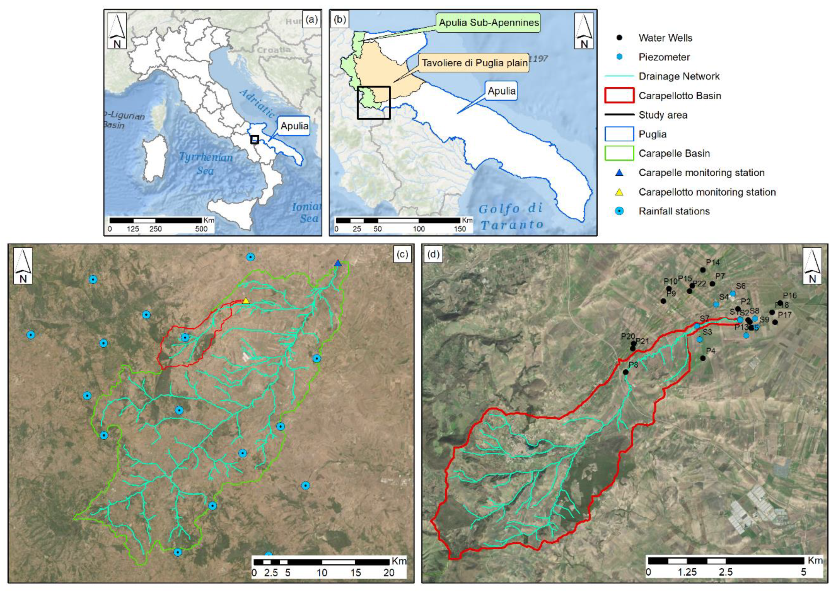
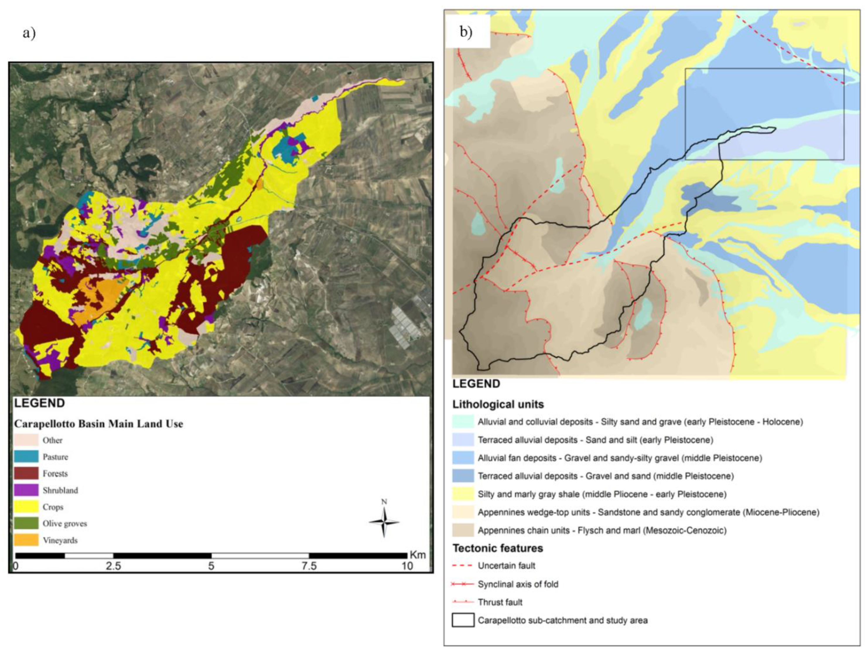
2.1. Study Area

The basin selected for setting up the experimental site is the Carapellotto (Figure 1d), which lies in the south-western sector of the Tavoliere di Puglia plain (Figure 1b). It includes the easternmost hills of the Sub-Apennines chain (Figure 1d) and the foothills area in the north-western part of the Apulia region (Southern Italy, Figure 1a). The drainage area is 27.17 km2, the elevation ranges from 226 to 1009 m a.s.l. with an average slope of 19.23% (Table 1). The climate, typically Mediterranean, influences the hydrological regime which is characterized by floods occurring mainly in the wet season (November/April) and by low flows in the dry season (May/October) [17]. The average yearly rainfall in the area, based on the data measured by the Department of Civil Protection (1921–2012), is 655 mm. The whole time series can be found at the following website: https://protezionecivile.puglia.it.
The basin is mainly covered with vegetation (more than 96%) [47]; the remaining is occupied by urban areas, roads, productive areas and rural buildings (Figure 2a). The predominant vegetation is agriculture (62%): Durum wheat and other non-irrigated crops cover 51%, while olive groves occupy 8%. Forests are in the upper part and on the hilly slopes (22% of total area), spontaneous vegetation and shrubs (12%) cover the riparian area of the drainage network. The lithology in the headwaters is characterized mainly by flysch-marly units and sandstone-sandy conglomerates. In the plain areas the main lithological classes are terraced silty-sand-gravel, alluvial deposits and silty-marly shale (Figure 2b).
The surroundings of the monitoring station (Figure 1), in the eastern sector of the area, are characterized by the presence of quaternary terraced alluvial deposits with very heterogeneous grain size and texture, that lie on the silty and marly clays referred to as the “Argille Subappennine Formation” (Plio-Pleistocene). In the Quaternary units lies the shallow porous aquifer of the Tavoliere di Puglia plain, a wide alluvial aquifer which represents the main source of the local water supply, mostly exploited for agricultural uses [48].
The Carapellotto is nested in the Carapelle basin, which is also monitored for runoff and SSC since 2007. More information about the Carapelle basin and its monitoring station can be found in Appendix A and in Gentile et al. [17].

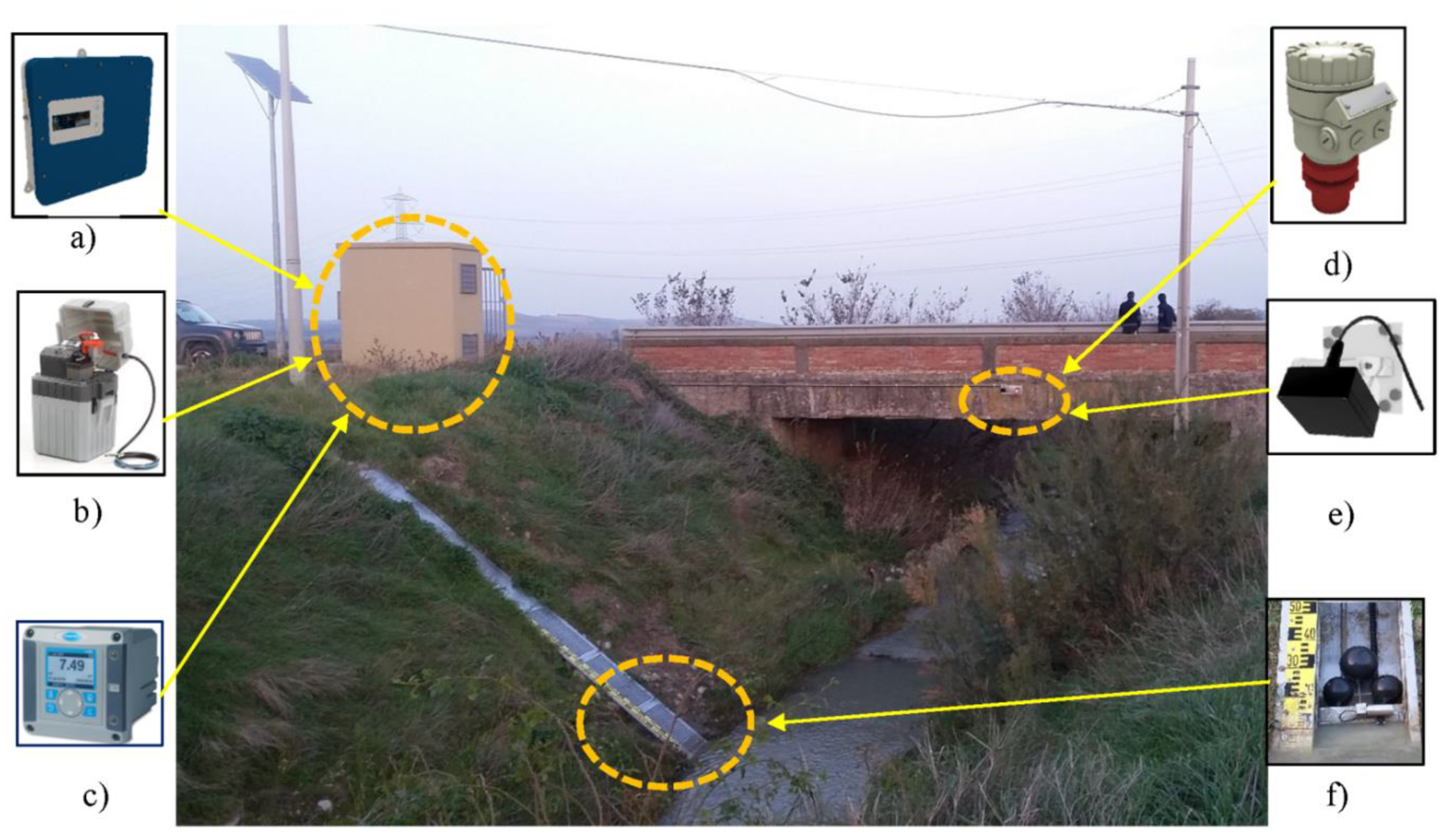
2.2. Monitoring Equipment and Data Analysis

In Apulia region (Southern Italy), the Italian Hydrographic Service used to manually sample SSC at 17 river cross-sections from 1951 to 1989; thereafter, it ceased such activity as it was time and cost expensive. In 2007, the Department of Agro-Environmental Science of Bari University installed a continuous SSC monitoring station on the Carapelle torrent (Ponte Ordona-Castelluccio dei Sauri, drainage area 506.2 km2), which worked from 2007 to 2011. The data obtained were used to analyze the sediment dynamics at the event scale [17,18,25], as well as to model erosion and transport processes [7,49,50].
To improve the knowledge of the sediment transport dynamics in the area and its relations with Q, a new measuring station for both Q and SSC was installed in the Carapellotto basin, nested in the Carapelle basin. In addition, a network of groundwater monitoring points was established in the areas surrounding the monitoring station, to improve the information about surface water-groundwater exchanges. In the following the data of the first year of activity are presented as well as the installation problems occurred during the study period. The Q–SSC relationship was investigated at the event scale through the hysteresis analysis. [51]. The analysis of the hysteretic loops considers that if the sediment peak SSCp occurs before the water discharge peak Qp, or if the SSC/Q ratios on the rising limb of the hydrograph (Q-graph) are greater than those on the falling limb, then the loop is clockwise. Instead, if SSCp arrives after Qp, or if SSC/Q ratios on the rising limb of the Q-graph are lower than those on the falling limb, the loop shows a counter-clockwise direction. The eight-shaped loop is a combination of a clockwise and a counter-clockwise loop, usually due to more than one peak in the hydrograph or sedigraph.
The surface flow-groundwater interdependence was assessed considering both the whole monitored period and at the event scale.
The monitoring station (Figure 3) installed in November 2015, includes a flow meter, a turbidimeter and an automatic sampler. A photovoltaic panel (24 V–240 Wp), located on a pole and equipped with a charge controller, provides the electricity to the system through two series-connected batteries (12 V–220 Ah). The electric panels, the instrument controllers, the flow and SSC data loggers and the automatic sampler are located in a prefabricated concrete cab.
The monitoring equipment is completed by an IP-Cam fixed to the bridge deck. The camera uses a Wi-Fi signal from a dedicated modem GSM/GPRS to upload every 15 min a snapshot to a ftp server. This enables the visual checking of the flood events and the status of the monitoring equipment.

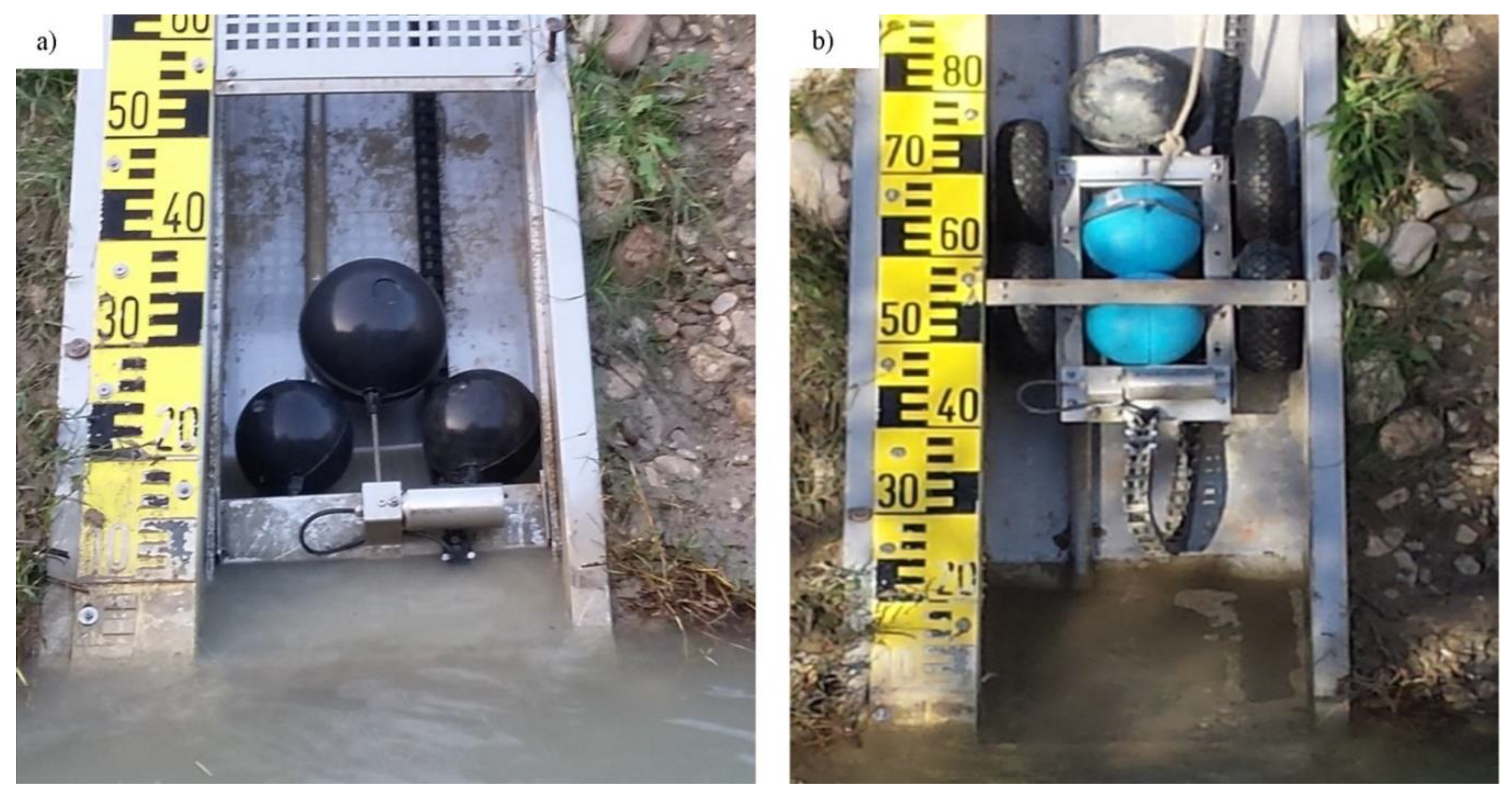
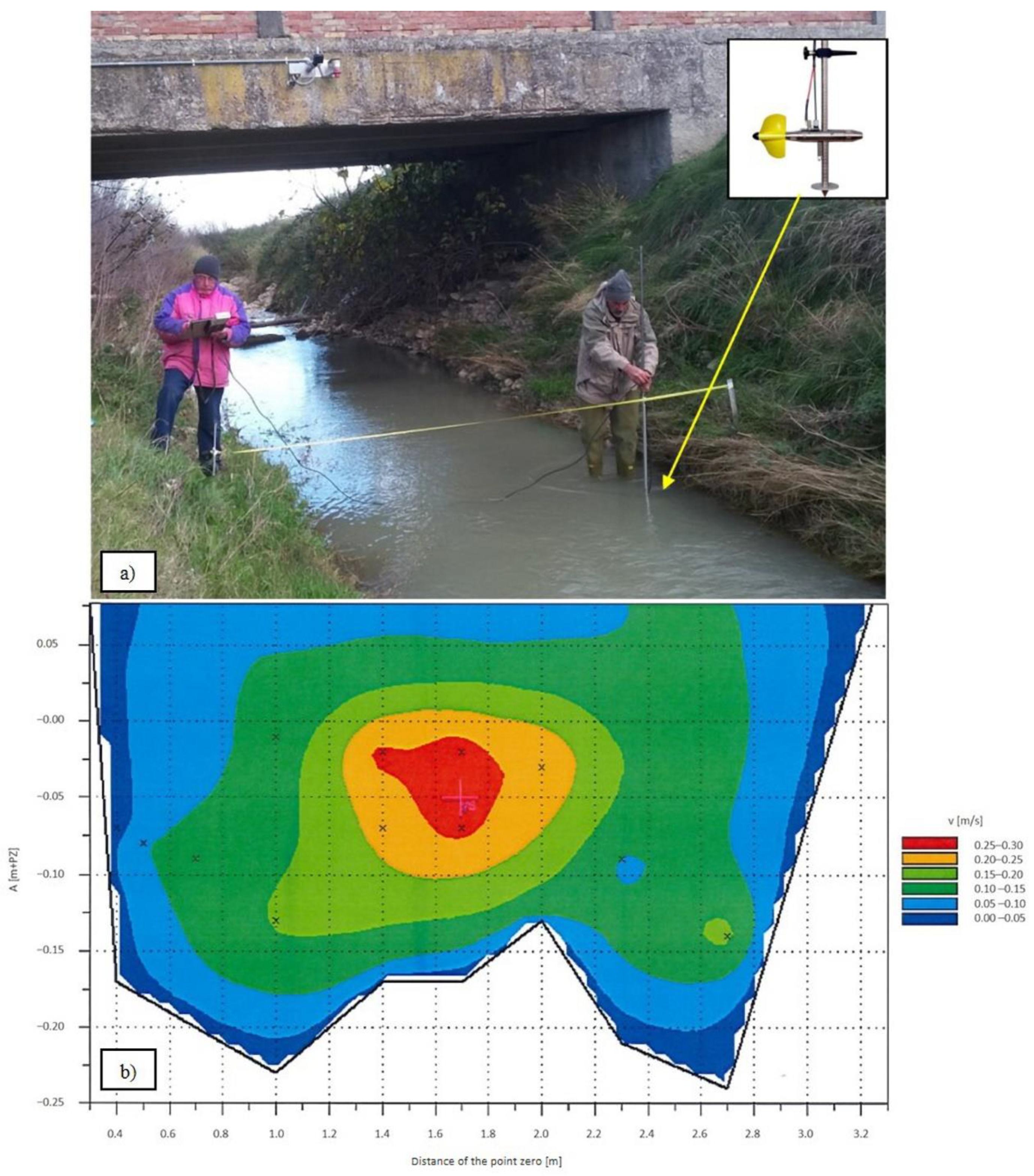
2.2.1. Water Discharge Measurement

The water discharge measurements are provided by a system composed of an ultrasonic sensor to measure the water level (Figure 3d), a radar sensor to measure the water surface velocity (Figure 3e) and a processor (Figure 3a) designed for operation and control of these sensors.
The discharge sensors are both installed on the upstream side of the bridge on the Carapellotto torrent, at about 3.5 m height from the bottom of the river. These non-contact measurements are elaborated by the processor applying the velocity-area method, assuming that the cross-section profile with trapezoid geometry is stable. The ultrasonic level sensor has a measuring range from 0.2 to 4 m with 0.2% accuracy. The radar velocity sensor (24 GHz) operates by means of the Doppler effect on the water surface. It ranges from 0.05 ms−1 to 15 ms−1, with 1 mms−1 resolution and 0.5% accuracy of the mean velocity reading. The time step for measuring with both instruments was set as 15 min. Finally, the processor is connected to an 8-channel data logger that manages and transmits data by means of a GSM/GPRS modem.
A field water discharge measurement was performed to calibrate sensors using a current meter (Figure 4a). In order to obtain the water discharge values all the recorded data of the velocity and water level were processed using SEBA Software-Q3 (Figure 4b).

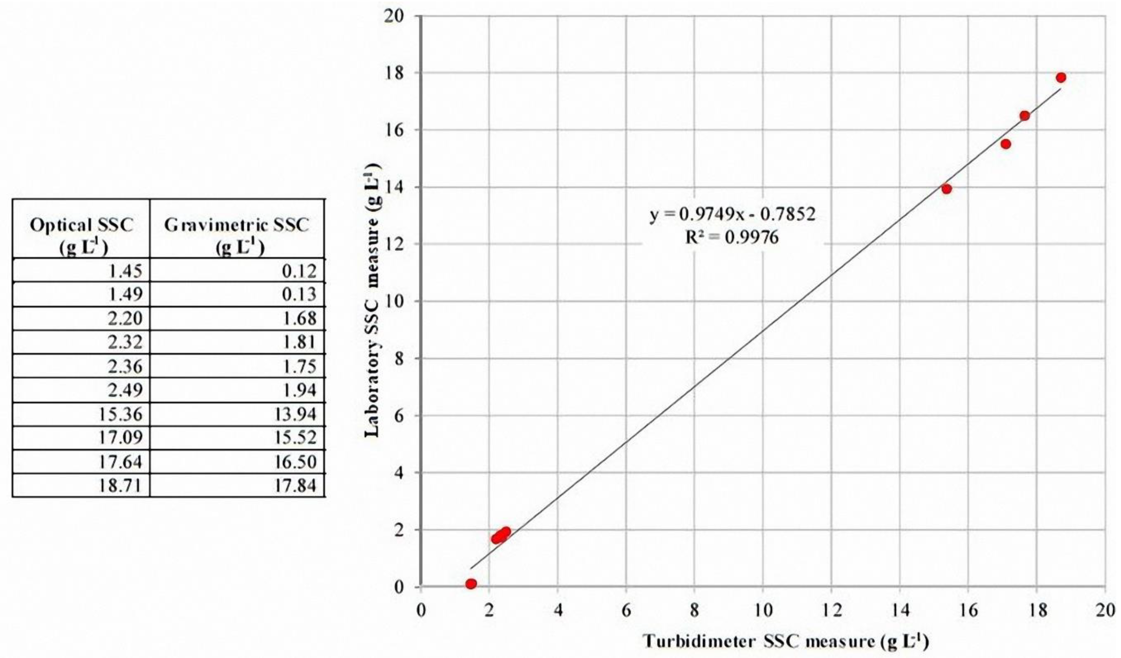
2.2.2. Suspended Sediment Concentration Measurement

Suspended solid concentration (SSC) measurements are performed by means of an optical sensor with dual-beam optics and a back-scatter detector both connected to the controller (Figure 3c). The optical probe is housed in a specific handmade metallic tank (width 0.5 m, height 0.4 m and length 6.1 m-Figure 3f), grilled from 0 to 1.60 m height and located on the western river bank. The sensor has the zero position at 0.15 m above the river bed and it is installed on a floating system (Figure 3f and Figure 8) in order to follow water level oscillations, measuring the sediment concentration close to the water surface. The housing tank permits the probe to float and protects it both from potential errors due to incident radiant energy straying into the infrared field and from impacts from coarse materials transported by floods.
The probe has a near infrared LED (light-emitting diode) light source that emits at an angle of 45°. Two photoreceptors detect scattered light, the first one at 90° (works when the turbidity method is selected) and the second backscatter at 140° (works when coupled with the first when the suspended solid concentration method is selected). The detectors measure the light emitted by the source beam and reflected by the suspended solids. A windscreen wiper activates every 15 min to clean the lens on the light emitter. These sensors are coupled to a dedicated controller that manages and displays the measured data. The controller allows two analog signal outputs (0–20 mA or 4–20 mA) and both of these can be set to represent a measured parameter. The output signals define a measurement range of 0.001–4000 NTU for turbidity mode and 0.001–50 g L−1 for suspended solids mode, assumed to be compatible with the expected characteristics of the sediment transport in the measuring section. The controller is connected to the 8-channel data logger that manages and transmits data by means of the GSM/GPRS modem.
The automatic sampler (Figure 3b) contains 24 bottles of 1 l capacity, and is located in the prefabricated cab, with a height of 4.3 m above the bottom of the river, while the pumping pipe is 10.5 m long. Aiming to refer the laboratory measurement to the same control volume as the turbidimeter measurement, the intake of the sampling pipe has been fixed on the turbidimeter floating system. An automatic sampler starts on a specific water level threshold and repeats sampling at established time intervals. Finally, to measure the water temperature in the river a temperature sensor has been installed within the housing tank (Figure 3f). The optical SSC values were calibrated against gravimetric SSC from 10 physical samples taken with dip-sampling [52] on 17 March and 3 May 2016 (Figure 5). The calibration equation of the turbidimeter fits the experimental data very well (Figure 5), with R2 = 0.99; furthermore, the uppermost gravimetric SSC is as high as 17.84 g L−1, which makes the equation quite reliable.

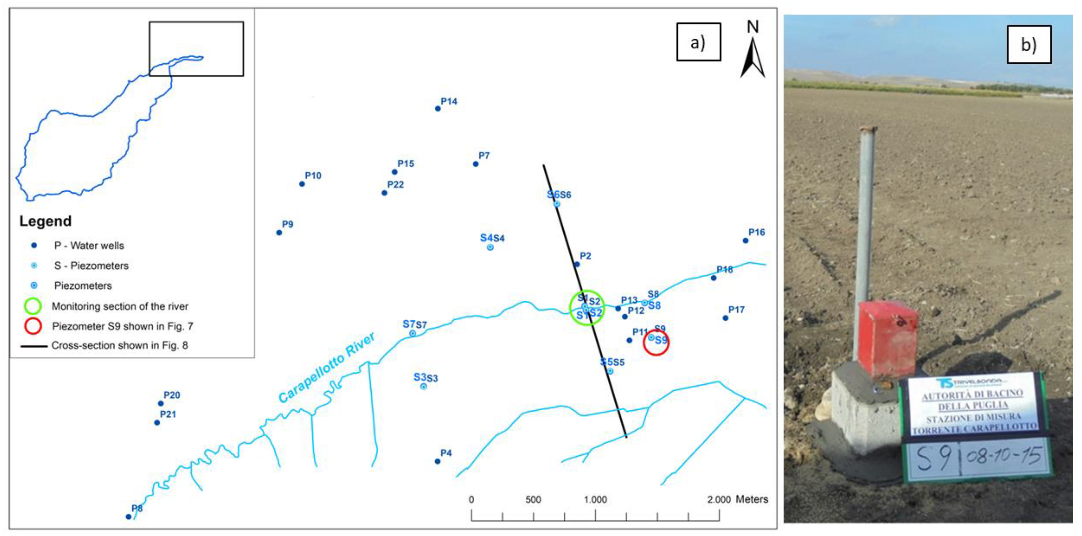
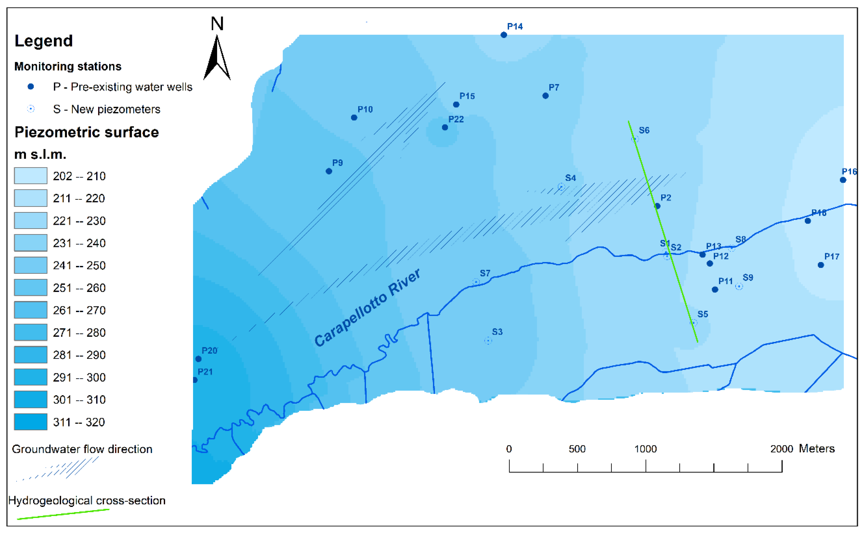
2.3. The Groundwater Monitoring Network

The groundwater monitoring network is based on nine new piezometers near to the river monitoring section and on several preexisting water wells. The two different groups differ in the spatial and temporal scale of the groundwater level measurements (Figure 6a).
A preliminary acquisition of piezometric data is provided by periodic measurements carried out every month in existing water wells surveyed with a portable piezometric probe, in order to provide a large-scale piezometric map around the monitoring section of the river and to estimate the groundwater flow direction and the seasonal regime of the water table. An integrated groundwater monitoring network has been designed in order to improve the distribution of the piezometric data and to better analyze the piezometric variation related to the hydraulic regime of the river. For this purpose, nine monitoring boreholes have been drilled and equipped with piezometric probes and data loggers for the continuous data recording (Figure 6b).
These monitoring wells are located along to the stream and at very short distances from it, not more than 1 km. They were drilled across the whole permeable thickness down to reach the underlying impervious clay substratum, so they are from 9 to 20 m deep. The boreholes’ stratigraphic data were recorded and analyzed to define the hydro-stratigraphic model of the study site. Slug tests were also carried out in two piezometers (S8 and S9) in order to estimate the hydraulic conductivity of the porous layers. All the piezometers (Sensor Technik Sirnach, STS) are equipped with piezometric probes consisting of pressure transducers, recording the water pressure and providing the height of the water column in the wells, with a +/− 0.05 % accuracy. The probes have selected sample rate from 0.5 s to 24 h, and they are all set to one-hour acquisition interval. Some of the piezometers closest to the river (S1, S3, S7 and S8) are also equipped with temperature probes (STS-OCS) in order to detect thermal impulses due to surface water/groundwater interactions, while the others (S2, S4, S5, S6 and S9) are equipped only with the piezometric probes (STS-DL70N).
Based on the stratigraphic logs from the boreholes S1, S2, S5 and S6 a hydro-stratigraphic cross-section oriented from N-NW to S-SE and passing through the river monitoring station was drawn (Figure 7). The analysis of the stratigraphic data recorded during the boreholes drilling revealed a wide variability in grain size and texture. All the data may be summarized in four main lithological units:
-
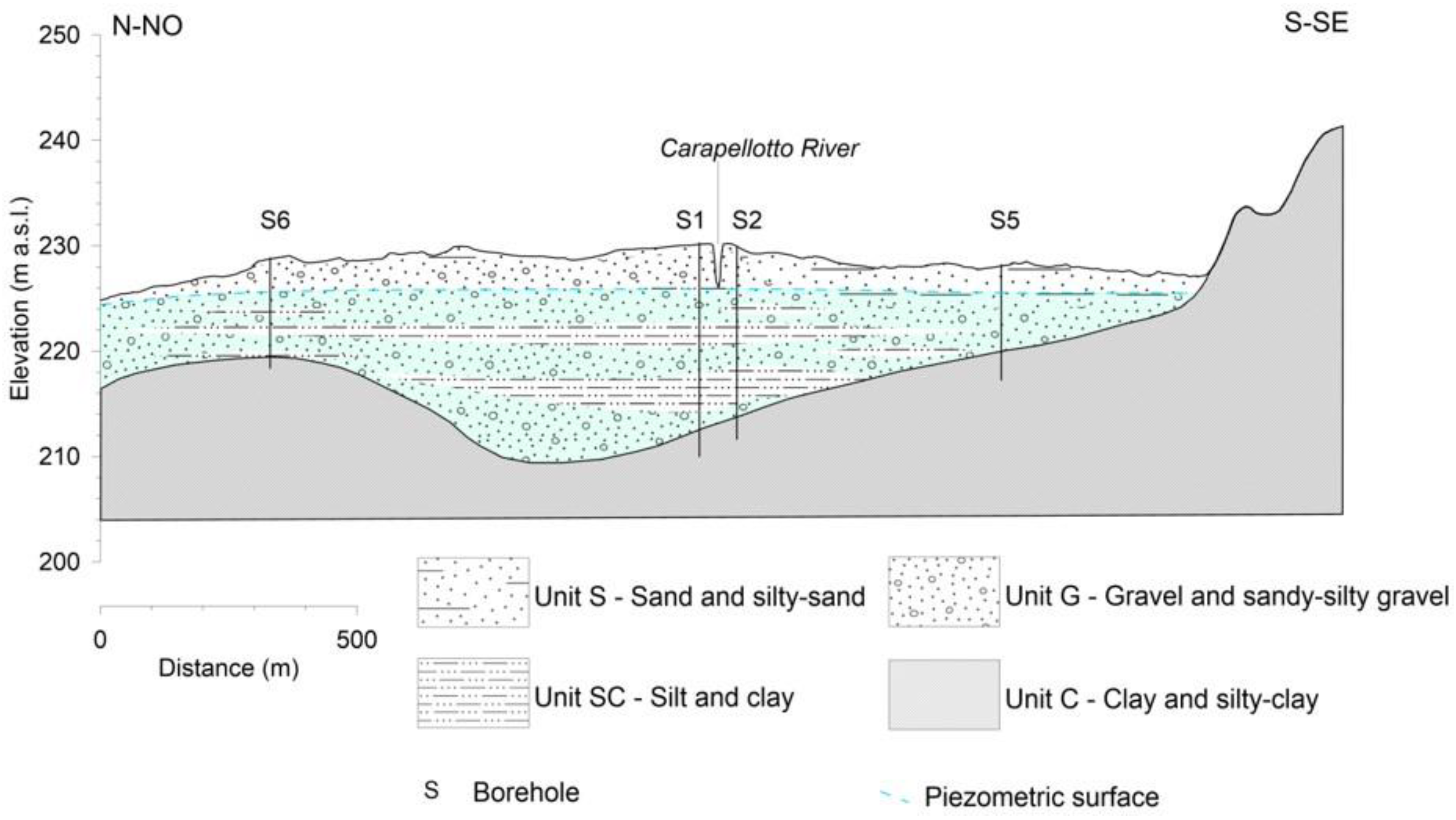
Unit S–Sand and silty sand;
-
Unit SC–Silt and clay;
-
Unit G–Gravel and sandy-silty gravel;
-
Unit C–Clay and silty-clay.
The spatial distribution of these lithologies in the subsoil is very complex, and it represents a typical expression of the fluvial sedimentary environment.
The subsoil is mainly characterized by clast-supported conglomerates and sandy-silty gravels referred to as the unit G, which is locally interbedded with silt and clay layers (Unit SC) at various depths. Sand and silty sand layers of the unit S are usually found on the top of the stratigraphic sequence, mainly on the right bank side, where they outcrop between the boreholes S2 and S5 and are up to 4 m thick. All these units are referred to the quaternary deposits, and they hold a very shallow aquifer.
The deeper unit (Unit C), composed of clay and silty clay, represents the uppermost level of the “Argille Subappennine” Formation. This unit outcrops on the hills surrounding the study site and it was also detected at the bottom of all the stratigraphic logs, at variable depth and roughly deepening from upstream to downstream. The top of the unit C is quite irregular, and it reflects the morphology of the ancient riverbed. Along the analyzed cross- section, it deepens from the S-SE hills to the central sector of the study area, passing from 8 m deep in S5 to 17 m deep in S1, while it rises up to 9 m of depth in S6.

3. Results and Discussion

3.1. Efficiency of the Monitoring Equipment

The monitoring site proved to be effective during its activity, thanks also to some modifications made compared to previous experiences. In particular, with respect to the Carapelle monitoring site, the implementation of the automatic sampler was very useful to get SSC data during floods, when it is very difficult to carry out a manual sampling [17,53]. These data, characterized by high SSC values, are very useful for the calibration of the turbidimeter (Figure 5). Moreover, getting samples is useful also to carry out studies focused on water quality [21], as the samples can be analyzed in the laboratory for nutrients and pesticides. With respect to other monitoring stations for water discharge and sediment load measurements [21,40] the inclusion of a network for the continuous monitoring of groundwater levels was effective to get information on the relationships among the different hydrological variables. Furthermore, the modular transmitter represents a mean not only to get data in real time but also to control if the monitoring equipment is correctly working, which is very important when the monitoring site is quite far and not very easy to reach. The camera enables a visual analysis of the flood events and of the status of the monitoring site.
As for the quality of the measurements, if the water discharge data are based on an accurate calibration on site (Figure 4), the turbidimeter data were validated with a laboratory analysis, which compared the optical SSC values against gravimetric SSC values with very high correlation (Figure 5). Moreover, the data coming from the piezometers were continuously checked and compared, for validation, with those coming from the monthly manual sampling in the wells.
In one year of monitoring, some installation problems affected only the SSC measurement equipment. According to Navratil et al. [54], failures are difficult to prevent before the test during floods. SSC was not successfully measured for four out of the eleven events that occurred (Table 2), caused by two mechanical problems. First, the sediment clogged the float guides, resulting in the blockage of the flotation system, which in turn caused the probe to be submerged by the sediment. Second, sediment also clogged the pumping pipe, causing failure of the automatic sampling.
The event nr. 2, which generated also the highest measured Qp, occurred in early spring, after a period of dry weather in which only a moderate event had occurred. The riverbed in the reach upstream the monitoring station was subjected to scouring, and a large amount of fine sediment reached the station. This caused failure of the monitoring system which prevented the measurement of SSC also for the event nr.3. After that, the housing tank, the turbidimeter and the automatic sampler pumping pipe were cleaned. From late spring to autumn, monitoring worked properly. After the dry period preceding event nr. 2, a constant flow was present in the channel also without a corresponding rainfall, highlighting the baseflow contribution.
In event nr. 10, the measurements were not reliable because, during the flood, the turbidimeter was blocked above the water level. Finally, in event nr. 11, the concentration measures failed, because it occurred in a period where the soil was bare, due to agricultural practices (wheat cultivation), making available a large amount of sediment which filled the lower part of the turbidimeter housing tank.
To fix the mechanical problems, the flotation system was redesigned (Figure 8a,b) by eliminating the sliding guides and putting in operation a support with dimensions similar to the cross-section of the housing tank. The inflatable wheels of the support permit free floating and limit excessive oscillations in the tank.

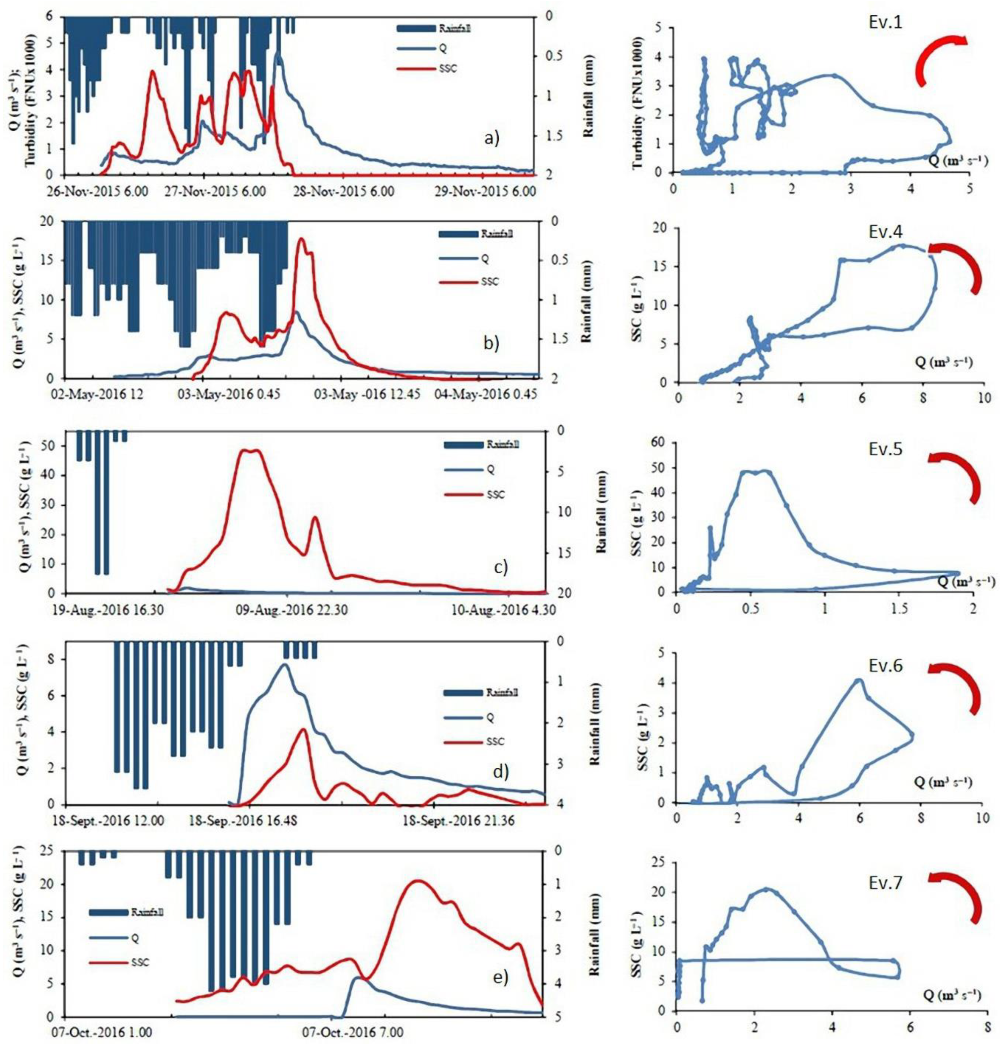
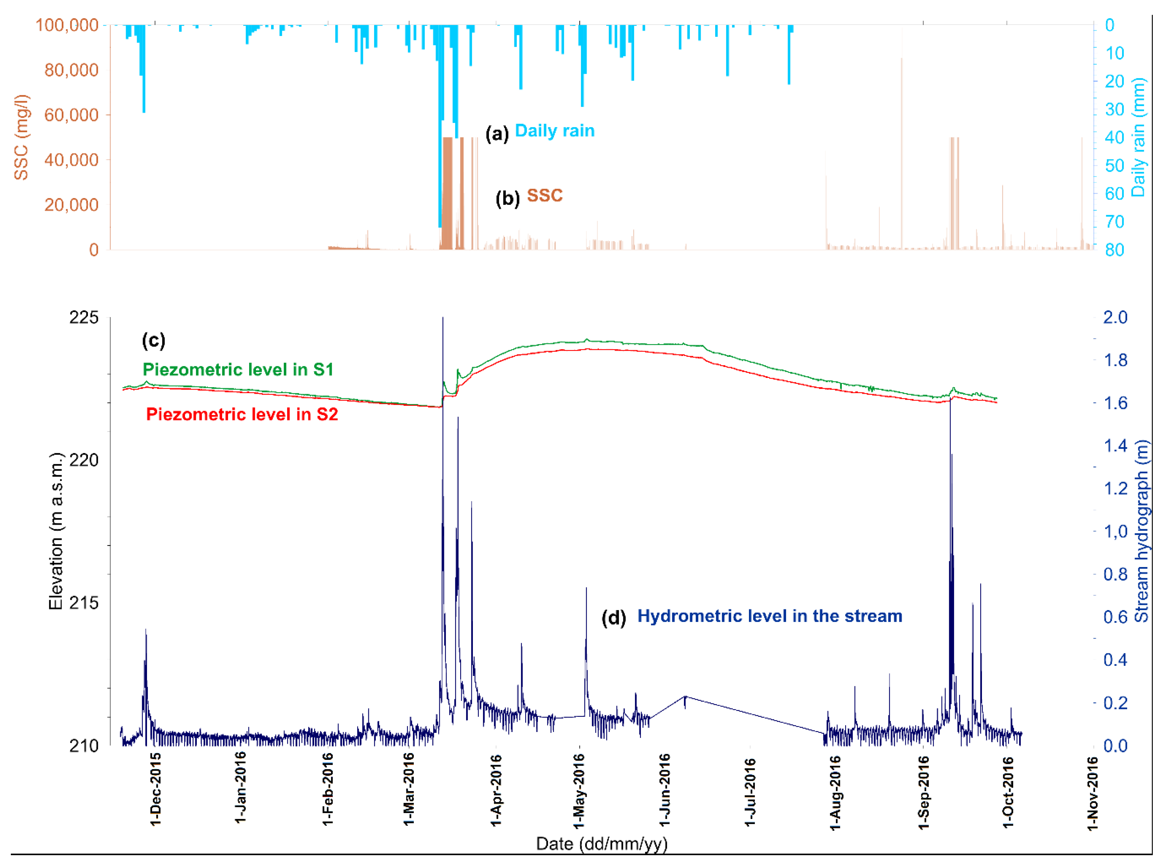
3.2. Water Discharge–Solid Concentration Patterns

The floods that showed efficient measurements of both water discharge and sediment concentration were analyzed (Table 2), plotting SSC-Q instantaneous values at the event scale. Five of them are reported as example in Figure 9.
The sedigraph of the event nr.1 reports turbidity values (FNU), because it occurred before the calibration of the turbidity sensor, while the others indicate SSC values (g L−1). Though the Carapellotto is a tributary of the Carapelle torrent, its maximum water discharge peak was 66.53 m3s−1 in the observation period, which is quite high if compared to the 159.50 m3s−1 in the Carapelle [18]. The concentration peaks, instead, were very similar, with 47.99 g L−1 for the Carapellotto, and 47.83 g L−1 for the Carapelle (Table 2). These comparisons confirm the key role of high-sloping sub-basins in fine sediment delivery to the whole river system [24,27,29,54,55,56,57]. Circular and eight-shaped hysteresis loops occurred, as well as clockwise and counter-clockwise. The essential features of the events are indicated in Table 2. Most of the analyzed events (events nr. 4, 5, 6, 7, 8, and 9), show that the counter-clockwise direction is predominant, during both circular and eight-shaped hysteresis, in accordance with the behavior of the whole Carapelle basin [18,51].
The only clockwise hysteresis was found for event nr. 1 occurred immediately after the equipment activation. This moderate event happened after the dry period June–November, finding a high sediment supply in non-covered soil conditions, which generated a clockwise hysteresis.
The Carapellotto seems to respond to the most commonly documented factors affecting small basins. In fact, several authors found that clockwise events may be more closely linked either to the speed of the initial delivery of sediment, together with the resuspension of in-channel fine sediment deposits [16], or to an early flushing of all available sediment in a connected stream network [2,14,21]. The scatter in the relation between suspended sediment concentrations and water discharge, as well as between the discharge peak and the lag of the concentration peak, is very high for the whole study period, indicating the variability of the sediment supply throughout the year of monitoring. SSC peak and Q peak appear to be weakly related (R² = 0.1656) during the monitoring year. Indeed, low values of Qp are associated with high values of SSCp. Generally, the suspended sediment transport processes depend on the location and activation of the sediment sources, as well as on their connectivity within the channel network [14,58] and are highly affected by land use conditions and the recent hydrological regime [17,59].
The Carapellotto behavior suggests, in accordance with De Girolamo et al. [21], that in-stream sediment transport is not strictly hydraulically driven, but rather it is predominantly controlled by sediment availability.

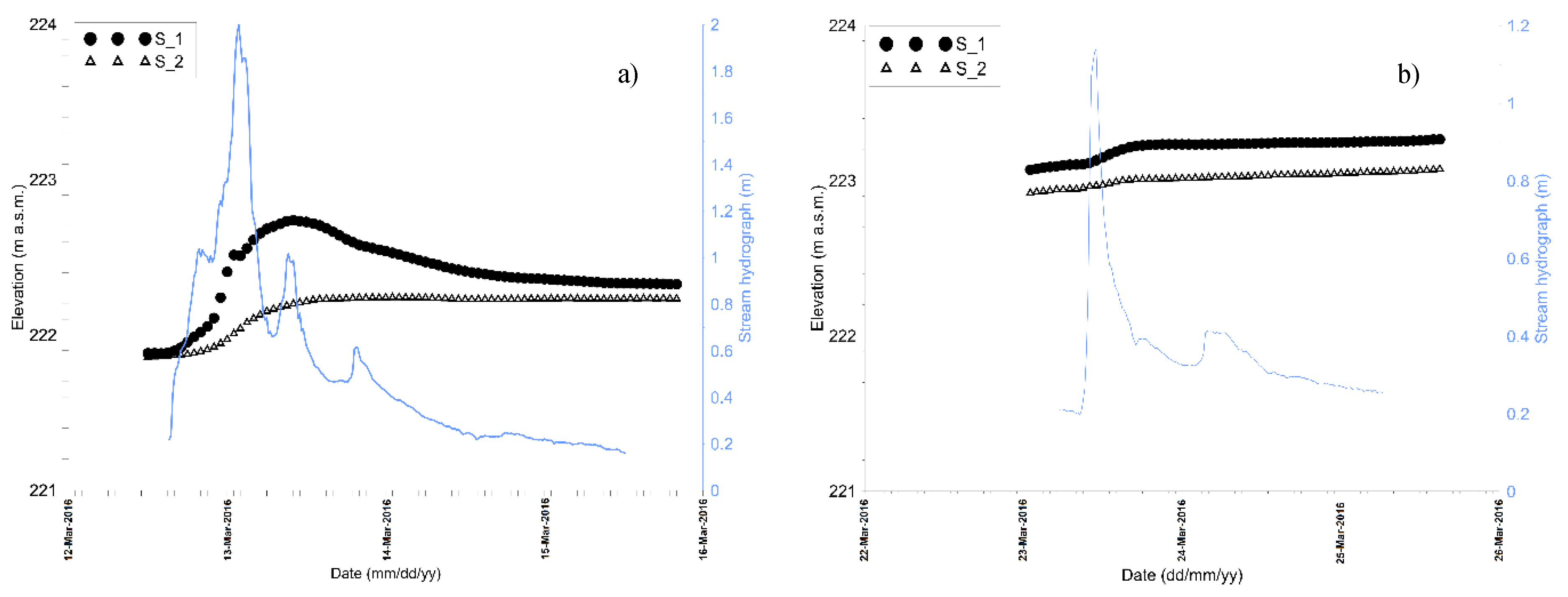
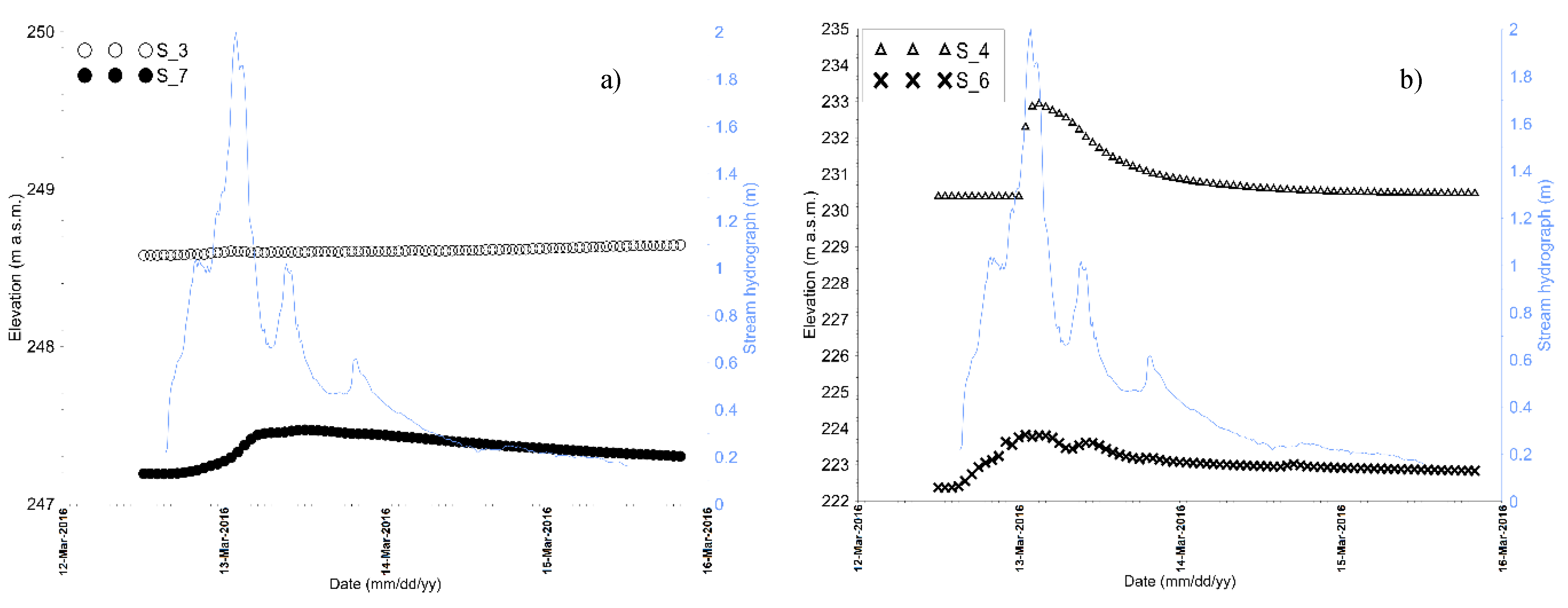
3.3. Hydrogeological and Hydrodynamic Characterization

The piezometric map (Figure 10) obtained by interpolating groundwater levels measured from the water wells and the boreholes shows a large range of variability, from about 295 m to 203 m a.s.l., according to the bottom aquifer behaviour.
The average hydraulic gradient is about 2%, although it varies all over the area, and it seems to define two main directions of the groundwater flow: The first roughly follows the Carapellotto river pattern, while the other appears to diverge toward the adjacent basin of the Cervaro river (Figure 10).
During the monitoring period, groundwater level variations were recorded in the wells, reaching maximum values during the spring season and the minimum in autumn, with different ranges of variability, from about 0.5 m to 3.5 m.
In general, the groundwater circulation is shallow. Close to the monitoring section, between the boreholes S1 and S2, it lies just below the river bed, so that the surface water in the river is directly connected with the shallow water table. On the one hand the surface water could recharge the shallow water table which rises up the river bed, on the other the shallow water table could contribute to the baseflow of the river [60].
The behavior of the groundwater level over time is provided by the continuous groundwater monitoring in the boreholes. In Figure 11 the pattern of the boreholes closest to the monitored cross-section (S1 and S2) is reported.
Analyzing the seasonal trend of the hydrological variables, during the period between December 2015 and March 2016 the scarcity of rain determines the progressive lowering of groundwater levels and the persistence of very low water levels in the torrent (Figure 11).
The occurrence of intense rainfall events in March 2016 reflects both on the water and groundwater levels, which show consistent peaks.
The groundwater level starts to increase quickly in March, with a growing amount of rain recorded in the area, it reaches the maximum value in April and, after a stationary period, it starts to decrease slowly from June to November. This trend represents the seasonal groundwater recharge mainly due to the river discharge, whose magnitude varies based on the location of the monitoring boreholes, as discussed later. In the following period, between April and June 2016, a persistence of the groundwater levels is observed as well as the presence of low flows in the stream even without rainfall events, which could be fed by groundwater [40]. In the same period quick and related responses of the water and groundwater levels to single rainfalls are also observed.
In Figure 11 the SSC values recorded in the monitoring period are also reported. In the same period April–June 2016 not negligible values of SSC are recorded, which could depend on the groundwater contribution to the baseflow of the stream, which could cause the re-suspension of the fine sediments deposited in the channel bed or the activation of in-channel erosion processes [22].
The piezometric curves related to S1 and S2, also show some local peaks strongly related to the flood events represented by the stream hydrograph. A detailed analysis of the most intense flood event (March 13, 2016) is reported in Figure 12. The groundwater level in S1 rises up to 0.8 m in a 20-h time interval, reaching the maximum value after 10 h from the flood peak and decreasing more slowly during the following 24 h. The behavior in S2 is quite different, since the maximum fluctuation of the groundwater level is lower than that recorded in S1 (about 0.4 m); after the peak, it does not decrease but it tends asymptotically to the same final value recorded in S1.
Although both piezometers are very close to the river and it is expected to have a similar behavior, the different response to the flood event is probably due to the local hydro-stratigraphic settings [36,61].
The cross-section reported in Figure 7 shows the presence of less permeable layers (aquitard) in the subsoil close to the monitoring station, confining a deeper aquifer layer by the perched water table below the river bed. All the aquifer layers are hydraulically interconnected one with the other, because of the local extension of the confining beds, although on the local scale the effects of the surface water and the groundwater interaction are detectable only in the uppermost aquifer levels. The screened section in S1 is in the uppermost part of the piezometer, so that the probe can detect the effect of the water exchange between the river and the groundwater that takes place in the shallower aquifer layers. On the contrary, in S2 the screened section of the piezometer is deeper than in S1, so the probe is less sensitive to the local variation related to the surface water/groundwater interaction.
Differences in magnitude and time lapse are recorded in most of the monitored boreholes, as shown in Figure 13.
In S7 (Figure 13a), which is located near the river and upstream of the monitoring section, a quite short fluctuation was recorded during the flood event and a gentler deplection curve in the following time period. In S3, located on the left bank of the river, the groundwater level seems to be insensitive to the flood effect, whereas in S4 and S6, which are located about 800 m away from the river, the highest fluctuation values are recorded, about 1.5 m and 2.5 m respectively with a very short response time (Figure 13b). These confirm what emerged by the analysis of S1 and S2. The pulses of the groundwater level depend on the intensity of the flood events, although they seem to be more sensible during flood events occurring after long drought periods, whereas they tend to fade during the recharge periods. In the event occurred on March 23 2016 (Figure 12b) the groundwater levels are almost at the maximum recorded values in S1 and S2. The flood peak recorded in terms of the stream stage is about 50 % of the previous event, the effects on the groundwater fluctuation are drastically reduced.

4. Conclusions

This study analyses the continuous monitoring of water discharge, suspended sediment concentration and groundwater levels in a Mediterranean basin, Southern Italy. During the period of observation, significant flood events occurred, offering useful information to improve the measuring equipment as well as to observe both the sediment dynamics and the surface water/groundwater interaction. This study confirms that turbidity measurements can represent a valid method for the continuous monitoring of SSC, however some failures have shown the necessity to improve the floating system to ensure, with the simplest possible equipment, functional robustness during floods. The Q and SSC peaks of the Carapellotto torrent are high compared with the values of the main Carapelle basin. This shows that headwater sub-basins could produce a significant fine sediment delivery to the whole river system. The analysis of the relationship between water discharge and SSC at the event scale shows counter-clockwise to be the predominant direction of the loops during both circular and eight-shaped hysteresis, according to the main Carapelle basin. The weak relationship between the SSC and Q peaks suggests that in the Carapellotto basin sediment availability and land-use conditions are the main factors controlling the suspended sediment transport processes.
The simultaneous monitoring of the groundwater and surface water levels provided interesting information on the hydraulic interaction between the stream and the aquifer. The data recorded show that the seasonal regime of groundwater is temporarily altered during flood events. Further analysis would better assess the relationship between water discharge and suspended sediment transport, as well as to evaluate the water transfer processes between the river and the aquifer during different flood conditions.

Author Contributions

Conceptualization: S.G.P., D.S. and F.G. Methodology: S.G.P., D.S. M.C., D.P., F.M., G.F.R. and F.G. Investigation: S.G.P., D.S. M.C. and D.P. Writing—original draft preparation: S.G.P. and D.S. Writing—review and editing: G.F.R. and F.G. Project administration: S.G.P. Funding acquisition: S.G.P. All authors have read and agreed to the published version of the manuscript.

Funding

The setting up of the Carapellotto site and the monitoring activities were founded with European funds PO-FESR 2007-2013 managed by Regione Puglia.

Acknowledgments

The authors acknowledge the Functional Centre of Civil Protection, Regione Puglia for providing the rainfall data. The authors would like to thank also the two anonymous reviewers for their constructive comments and suggestions.

Conflicts of Interest

The authors declare no conflict of interest.

Appendix A

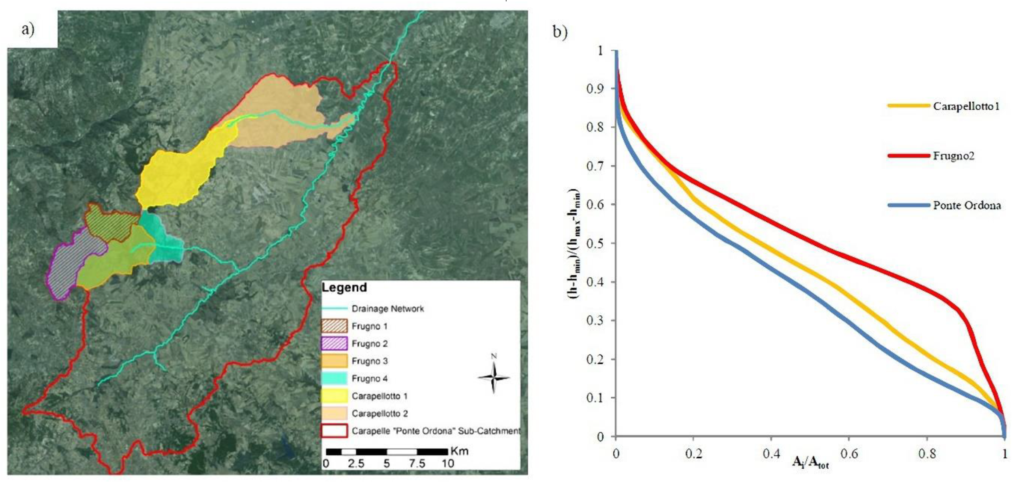
The Carapelle Basin and the Selection of the Nested Monitoring Basin

The Carapelle stream is one of the main torrents in the northern part of the Apulia region. It comes from the Apennines in Campania and, after crossing the areas of Subappennine, runs along the flood plain of the Tavoliere to its natural mouth in the south-central Gulf of Manfredonia. The total drainage area of the basin is 831 km2.
Since 1989, the only active monitoring station to measure the SSC in the Apulia region is located on the main channel of the Carapelle torrent in the locality of Ponte Ordona-Castelluccio dei Sauri. The drainage area of this basin is 506.2 km2 (Figure 1) and the main morphometric characteristics are summarized in Table A1.
The Functional Centre of the Apulia Region Civil Protection monitors continuously the water flows through an ultrasonic stage sensor that transmits data in telemetry, a traditional electro-mechanical stage meter and a cableway. For the continuous measurement of turbidity, in 2007 the Di.S.A.A.T Department installed an optical infrared probe. Laboratory and field tests were used to link suspended sediment concentration and turbidity. The instrument is housed in a perforated pipe to protect it from the impact of the coarse material carried by the flow and to prevent measurement errors caused by natural radiation in the infrared range. Today, quite a long data series is available (2007–2011).
Apennine units widely outcrop in the middle and western sector of the basin area, characterized by marl and flysch sequences more exposed to erosion, whereas in the eastern sector quaternary lithological units outcrop, represented by debris flow and coarse-grained sediments deposited in alluvial fan settings, passing eastward to gravel and sand-gravel deposited in a braided alluvial plain. The heterogeneity of the Quaternary deposits has effects on the variability of the hydrogeological characteristics of the subsoil. Considering the hydro-stratigraphic setting of the area, the shallow alluvial aquifer consists of a complex alternation of gravel, sand and sandy-loamy sediments frequently interbedded, resulting in a multi-layered aquifer whose bottom is always represented by the top of the “Argille Subappennine” Formation. The Lefranc tests carried out in some of the boreholes provided permeability values for the unit G varying from 8.24×10⁻⁶ m s−1 to 6.59×10⁻⁷ m s−1 as the sandy and loamy matrix increases. Moreover, the spatial distribution and thickness of the units S and SC sensibly affect the hydraulic transmissivity of the aquifer. The unit C represents the impervious substratum for the aquifer and its top morphology may have effects on the groundwater hydraulic gradient and flow direction and it could delineate a groundwater divide that is not always aligned to the surface basin (Figure 7). Land use is mainly agricultural, with plains and low hills used for wheat and olive groves, while at higher altitudes there are predominantly woods and pasture activities. The climate is typically Mediterranean. At the various rainfall stations located in the basin, the yearly precipitation ranges from 450 to 800 mm, while the average annual temperature ranges between 10 and 16 °C.
Table A1. Morphologic features of Carapelle catchment.
Area (km2)506.2
Perimeter (km)141.7
Minimum elevation (m a.s.l.)112
Maximum elevation (m a.s.l.)1094
Gravelius Index1.78
Catchment average slope (%)15
Length of main channel (km)65.98
Average width of main channel (m)9.6
Average slope of main channel (%)12.1
Average annual precipitation (mm)450÷800
Mean annual temperature (°C)10÷16
To choose the new sub-basin to be monitored, after the preliminary cartographic selection, two left tributaries of the Carapelle torrent were examined, as shown in Figure A1a: the Frugno torrent and the Carapellotto torrent. Four cross-sections for the Frugno torrent and two cross-sections for the Carapellotto torrent and their associated basins were analyzed (Table A1).
Figure A1. Sub-basins candidate to be gauged (a) and hypsometric curves with significant similarity (b).
Water 12 03130 g0a1
To make the SSC characteristics of the new sub basin comparable with those of the Carapelle basin, the selected sub-basin to monitor should show a similar maturity state in the measuring section. In Figure A1b, the comparison between the hypsometric curves shows that “Carapellotto 1” is the closest to the main basin in terms of its state of maturity.
The “Carapellotto 1” section was also selected because of the absence of hydraulic interference in the stream, the presence of a bridge and a straight river stretch which are favorable features to convey the extreme peak flows.
A 500 years’ flow was assumed to verify that the instruments were not washed by the flood, while the Soil Conservation Service curve number (SCS-CN) method was used to generate the flood hydrograph.
The flood generation was simulated by performing a distributed parameters model in unsteady flow with one-dimensional (1D) and two-dimensional (2D) domains using TUFLOW (Two-dimensional Unsteady FLOW) software with an SMS interface.
Table A2. Sub-basins candidate to be gauged and main morphologic features.
Basin NameArea (km2)Basin Average Slope (%)Minimum Elevation
(m a.s.l.)
Maximum Elevation
(m a.s.l.)
Average Elevation
(m a.s.l.)
Main Channel Lenght
(km)
Carapellotto127.1719.232261009548.8216.21
Carapellotto263.4710.981501009362.2225.34
Frugno18.5927.465231094768.334.99
Frugno213.4521.135581015784.218.45
Frugno338.3923.944221094720.9415.74
Frugno446.8824.71361.001094.0069718.85

References

  1. De Boer, D.H.; Campbell, I.A. Spatial scale dependence of sediment dynamics in a semi-arid badland drainage basin. Catena 1989, 16, 277–290. [Google Scholar] [CrossRef]
  2. Seeger, M.; Errea, M.P.; Beguería, S.; Arnáez, J.; Martí, C.; García-Ruiz, J.M. Catchment soil moisture and rainfall characteristics as determinant factors for discharge/suspended sediment hysteretic loops in a small headwater catchment in the Spanish pyrenees. J. Hydrol. 2004, 288, 299–311. [Google Scholar] [CrossRef] [Green Version]
  3. Soler, M.; Latron, J.; Gallart, F. Relationships between suspended sediment concentrations and discharge in two small research basins in a mountainous Mediterranean area (Vallcebre, Eastern Pyrenees). Geomorphology 2008, 98, 143–152. [Google Scholar] [CrossRef]
  4. Luetzenburg, G.; Bittner, M.J.; Calsamiglia, A.; Renschler, C.S.; Estrany, J.; Poeppl, R. Climate and land use change effects on soil erosion in two small agricultural catchment systems Fugnitz–Austria, Can Revull–Spain. Sci. Total Environ. 2020, 704, 135389. [Google Scholar] [CrossRef]
  5. Vogel, R.M.; Stedinger, J.R.; Hooper, R.P. Discharge indices for water quality loads. Water Resour. Res. 2003, 39. [Google Scholar] [CrossRef] [Green Version]
  6. Steiger, J.; Gurnell, A.M.; Petts, G.E. Sediment deposition along the channel margins of a reach of the middle River Severn, UK. Regul. Rivers Res. Manag. 2001, 17, 443–460. [Google Scholar] [CrossRef]
  7. Gentile, F.; Bisantino, T.; Trisorio Liuzzi, G. Erosion and sediment transport modelling in Northern Puglia watersheds. In Proceedings of the WIT Transactions on Engineering Sciences; WIT Press: Southampton, UK, 2010; Volume 67, pp. 199–212. [Google Scholar]
  8. López-Tarazón, J.A.; Batalla, R.J.; Vericat, D.; Francke, T. The sediment budget of a highly dynamic mesoscale catchment: The River Isábena. Geomorphology 2012, 138, 15–28. [Google Scholar] [CrossRef]
  9. Ricci, G.F.; Jeong, J.; De Girolamo, A.M.; Gentile, F. Effectiveness and feasibility of different management practices to reduce soil erosion in an agricultural watershed. Land Use Policy 2020, 90, 104306. [Google Scholar] [CrossRef]
  10. Walling, D.E.; Fang, D. Recent trends in the suspended sediment loads of the world’s rivers. Glob. Planet. Chang. 2003, 39, 111–126. [Google Scholar] [CrossRef]
  11. De Girolamo, A.M.; Di Pillo, R.; Lo Porto, A.; Todisco, M.T.; Barca, E. Identifying a reliable method for estimating suspended sediment load in a temporary river system. Catena 2018, 165, 442–453. [Google Scholar] [CrossRef]
  12. Downing, J. Twenty-five years with OBS sensors: The good, the bad, and the ugly. Cont. Shelf Res. 2006, 26, 2299–2318. [Google Scholar] [CrossRef]
  13. Bhamjee, R.; Lindsay, J.B. Ephemeral stream sensor design using state loggers. Hydrol. Earth Syst. Sci. 2011, 15, 1009–1021. [Google Scholar] [CrossRef] [Green Version]
  14. Brasington, J.; Richards, K. Turbidity and suspended sediment dynamics in small catchments in the Nepal Middle Hills. Hydrol. Process. 2000, 14, 2559–2574. [Google Scholar] [CrossRef]
  15. Zabaleta, A.; Martínez, M.; Uriarte, J.A.; Antigüedad, I. Factors controlling suspended sediment yield during runoff events in small headwater catchments of the Basque Country. Catena 2007, 71, 179–190. [Google Scholar] [CrossRef]
  16. Smith, H.G.; Dragovich, D. Interpreting sediment delivery processes using suspended sediment-discharge hysteresis patterns from nested upland catchments, south-eastern Australia. Hydrol. Process. 2009, 23, 2415–2426. [Google Scholar] [CrossRef]
  17. Gentile, F.; Bisantino, T.; Corbino, R.; Milillo, F.; Romano, G.; Trisorio Liuzzi, G. Monitoring and analysis of suspended sediment transport dynamics in the Carapelle torrent (Southern Italy). Catena 2010, 80, 1–8. [Google Scholar] [CrossRef]
  18. García-Rama, A.; Pagano, S.G.; Gentile, F.; Lenzi, M.A. Suspended sediment transport analysis in two Italian instrumented catchments. J. Mt. Sci. 2016, 13, 957–970. [Google Scholar] [CrossRef]
  19. Klein, M. Anti clockwise hysteresis in suspended sediment concentration during individual storms: Holbeck catchment; Yorkshire, England. Catena 1984, 11, 251–257. [Google Scholar] [CrossRef]
  20. Jansson, M.B. Determining sediment source areas in a tropical river basin, Costa Rica. Catena 2002, 47, 63–84. [Google Scholar] [CrossRef]
  21. De Girolamo, A.M.; Pappagallo, G.; Lo Porto, A. Temporal variability of suspended sediment transport and rating curves in a Mediterranean river basin: The Celone (SE Italy). Catena 2015, 128, 135–143. [Google Scholar] [CrossRef]
  22. Eder, A.; Exner-Kittridge, M.; Strauss, P.; Blöschl, G. Re-suspension of bed sediment in a small stream-results from two flushing experiments. Hydrol. Earth Syst. Sci. 2014, 18, 1043–1052. [Google Scholar] [CrossRef] [Green Version]
  23. Williams, G. Sediment concentration versus water discharge during single hydrologic events in rivers. J. Hydrol. 1989, 111, 89–106. [Google Scholar] [CrossRef]
  24. Navratil, O.; Esteves, M.; Legout, C.; Gratiot, N.; Nemery, J.; Willmore, S.; Grangeon, T. Global uncertainty analysis of suspended sediment monitoring using turbidimeter in a small mountainous river catchment. J. Hydrol. 2011, 398, 246–259. [Google Scholar] [CrossRef]
  25. Fortesa, J.; Ricci, G.F.; García-Comendador, J.; Gentile, F.; Estrany, J.; Sauquet, E.; Datry, T.; De Girolamo, A.M. Analysing hydrological and sediment transport regime in two Mediterranean intermittent rivers. Catena 2020, 196, 104865. [Google Scholar] [CrossRef]
  26. Gippel, C.J. Potential of turbidity monitoring for measuring the transport of suspended solids in streams. Hydrol. Process. 1995, 9, 83–97. [Google Scholar] [CrossRef]
  27. Mathys, N.; Brochot, S.; Meunier, M.; Richard, D. Erosion quantification in the small marly experimental catchments of Draix (Alpes de Haute Provence, France). Calibration of the ETC rainfall-runoff-erosion model. Catena 2003, 50, 527–548. [Google Scholar] [CrossRef]
  28. Orwin, J.F.; Smart, C.C. An inexpensive turbidimeter for monitoring suspended sediment. Geomorphology 2005, 68, 3–15. [Google Scholar] [CrossRef]
  29. Mano, V.; Nemery, J.; Belleudy, P.; Poirel, A. Assessment of suspended sediment transport in four alpine watersheds (France): Influence of the climatic regime. Hydrol. Process. 2009, 23, 777–792. [Google Scholar] [CrossRef]
  30. Felix, D.; Albayrak, I.; Boes, R.M. Field measurements of suspended sediment using several methods. In Proceedings of the E-Proceedings 36th IAHR World Congress, Hague, The Netherlands, 28 June–3 July 2015. [Google Scholar]
  31. García-Comendador, J.; Fortesa, J.; Calsamiglia, A.; Calvo-Cases, A.; Estrany, J. Post-fire hydrological response and suspended sediment transport of a terraced Mediterranean catchment. Earth Surf. Process. Landforms 2017, 42, 2254–2265. [Google Scholar] [CrossRef]
  32. Winter, T.C.; Harvey, J.W.; Lehn Franke, O.; Alley, M.W. Ground Water and Surface Water: A Single Resource. Available online: https://www.researchgate.net/publication/243787829_Ground_water_and_surface_water_a_single_resource_U (accessed on 7 October 2020).
  33. Woessner, W.W. Stream and fluvial plain ground water interactions: Rescaling hydrogeologic thought. Ground Water 2000, 38, 423–429. [Google Scholar] [CrossRef]
  34. Brodie, R.; Sundaram, B.; Tottenham, R.; Hostetler, S.; Ransley, T. An Overview of Tools for Assessing Groundwater-Surface Water Connectivity; Australian Government, Bureau of Rural Sciences: Canberra, Australia, 2007. [Google Scholar]
  35. Squillace, P.J. Observed and Simulated Movement of Bank-Storage Water. Ground Water 1996, 34, 121–134. [Google Scholar] [CrossRef]
  36. Siergieiev, D.; Ehlert, L.; Reimann, T.; Lundberg, A.; Liedl, R. Modelling hyporheic processes for regulated rivers under transient hydrological and hydrogeological conditions. Hydrol. Earth Syst. Sci. 2015, 19, 329–340. [Google Scholar] [CrossRef] [Green Version]
  37. Kattan, Z.; Gac, J.Y.; Probst, J.L. Suspended sediment load and mechanical erosion in the Senegal Basin-Estimation of the surface runoff concentration and relative contributions of channel and slope erosion. J. Hydrol. 1987, 92, 59–76. [Google Scholar] [CrossRef]
  38. Andermann, C.; Bonnet, S.; Crave, A.; Davy, P.; Longuevergne, L.; Gloaguen, R. Sediment transfer and the hydrological cycle of Himalayan rivers in Nepal. Comptes Rendus-Geosci. 2012, 344, 627–635. [Google Scholar] [CrossRef]
  39. Ayes Rivera, I.; Callau Poduje, A.C.; Molina-Carpio, J.; Ayala, J.M.; Armijos Cardenas, E.; Espinoza-Villar, R.; Espinoza, J.C.; Gutierrez-Cori, O.; Filizola, N. On the Relationship between Suspended Sediment Concentration, Rainfall Variability and Groundwater: An Empirical and Probabilistic Analysis for the Andean Beni River, Bolivia (2003–2016). Water 2019, 11, 2497. [Google Scholar] [CrossRef] [Green Version]
  40. Estrany, J.; Garcia, C.; Batalla, R.J. Groundwater control on the suspended sediment load in the Na Borges River, Mallorca, Spain. Geomorphology 2009, 106, 292–303. [Google Scholar] [CrossRef]
  41. McCallum, J.L.; Cook, P.G.; Berhane, D.; Rumpf, C.; McMahon, G.A. Quantifying groundwater flows to streams using differential flow gaugings and water chemistry. J. Hydrol. 2012, 416–417, 118–132. [Google Scholar] [CrossRef]
  42. Yang, Z.; Zhou, Y.; Wenninger, J.; Uhlenbrook, S. Une approche pluridisciplinaire pour quantifier les interactions eau superficielle-eau souterraine dans le bassin semi-aride de la rivière Hailiutu, Nord-Ouest de la Chine. Hydrogeol. J. 2014, 22, 527–541. [Google Scholar] [CrossRef]
  43. Gao, F.; Feng, G.; Han, M.; Dash, P.; Jenkins, J.; Liu, C. Assessment of Surface Water Resources in the Big Sunflower River Watershed Using Coupled SWAT–MODFLOW Model. Water 2019, 11, 528. [Google Scholar] [CrossRef] [Green Version]
  44. Fattorelli, S.; Lenzi, M.; Marchi, L.; Keller, H.M. Une station expérimentale pour l’enregistrement automatique du débit de l’eau et du transport de sédiments dans un petit bassin versant alpin. Hydrol. Sci. J. 1988, 33, 607–617. [Google Scholar] [CrossRef] [Green Version]
  45. Fortesa, J.; García-Comendador, J.; Calsamiglia, A.; López-Tarazón, J.A.; Latron, J.; Alorda, B.; Estrany, J. Comparison of stage/discharge rating curves derived from different recording systems: Consequences for streamflow data and water management in a Mediterranean island. Sci. Total Environ. 2019, 665, 968–981. [Google Scholar] [CrossRef]
  46. Han, K.; Zhang, D.; Bo, J.; Zhang, Z. Hydrological Monitoring System Design and Implementation Based on IOT. Phys. Procedia 2012, 33, 449–454. [Google Scholar] [CrossRef] [Green Version]
  47. Aquilino, M.; Novelli, A.; Tarantino, E.; Iacobellis, V.; Gentile, F. Evaluating the potential of GeoEye data in retrieving LAI at watershed scale. In Proceedings of the Remote Sensing for Agriculture, Ecosystems, and Hydrology XVI; Neale, C.M.U., Maltese, A., Eds.; SPIE: Bellingham, WA, USA, 2014; Volume 9239, p. 92392B. [Google Scholar]
  48. Passarella, G.; Barca, E.; Sollitto, D.; Masciale, R.; Bruno, D.E. Cross-Calibration of Two Independent Groundwater Balance Models and Evaluation of Unknown Terms: The Case of the Shallow Aquifer of BTavoliere di Puglia^ (South Italy). Water Resour. Manag. 2016, 31, 327–340. [Google Scholar] [CrossRef]
  49. Bisantino, T.; Gentile, F.; Milella, P.; Liuzzi, G.T. Effect of Time Scale on the Performance of Different Sediment Transport Formulas in a Semiarid Region. J. Hydraul. Eng. 2010, 136, 56–61. [Google Scholar] [CrossRef]
  50. Abdelwahab, O.M.M.; Bingner, R.L.; Milillo, F.; Gentile, F. Evaluation of Alternative Management Practices with the AnnAGNPS Model in the Carapelle Watershed. Soil Sci. 2016, 181, 293–305. [Google Scholar] [CrossRef]
  51. Pagano, S.G.; Rainato, R.; García-Rama, A.; Gentile, F.; Lenzi, M.A. Analysis of suspended sediment dynamics at event scale: Comparison between a mediterranean and an alpine basin. Hydrol. Sci. J. 2019, 64, 948–961. [Google Scholar] [CrossRef]
  52. Edwards, T.K.; Douglas, G.G. Field Methods for Measurement of Fluvial Sediment. [Rev.] ed., Techniques for Water-Resources Investigations of the United States Geological Survey; U.S. Geological Survey, Techniques of Water-Resources Investigations: Denver, CO, USA, 1999. [Google Scholar]
  53. Gentile, F.; Bisantino, T.; Corbino, R.; Milillo, F.; Romano, G.; Trisorio Liuzzi, G. Sediment transport monitoring in a Northern Puglia watershed. In Proceedings of the WIT Transactions on Engineering Sciences; WIT Press: Southampton, UK, 2008; Volume 60, pp. 153–161. [Google Scholar]
  54. Navratil, O.; Legout, C.; Gateuille, D.; Esteves, M.; Liebault, F. Assessment of intermediate fine sediment storage in a braided river reach (southern French Prealps). Hydrol. Process. 2010, 24, 1318–1332. [Google Scholar] [CrossRef]
  55. Milliman, J.D.; Syvitski, J.P.M. Geomorphic/tectonic control of sediment discharge to the ocean: The importance of small mountainous rivers. J. Geol. 1992, 100, 525–544. [Google Scholar] [CrossRef]
  56. Hicks, D.M.; Gomez, B.; Trustrum, N.A. Erosion thresholds and suspended sediment yields, Waipaoa River Basin, New Zealand. Water Resour. Res. 2000, 36, 1129–1142. [Google Scholar] [CrossRef]
  57. Meybeck, M.; Laroche, L.; Dürr, H.; Syvitski, J.P. Global variability of daily total suspended solids and their fluxes in rivers. Glob. Planet. Chang. 2003, 39, 65–93. [Google Scholar] [CrossRef]
  58. Aich, V.; Zimmermann, A.; Elsenbeer, H. Quantification and interpretation of suspended-sediment discharge hysteresis patterns: How much data do we need? Catena 2014, 122, 120–129. [Google Scholar] [CrossRef]
  59. Turowski, J.M.; Rickenmann, D.; Dadson, S.J. The partitioning of the total sediment load of a river into suspended load and bedload: A review of empirical data. Sedimentology 2010, 57, 1126–1146. [Google Scholar] [CrossRef]
  60. McDonough, O.T.; Hosen, J.; Palmer, M. Temporary streams: The hydrology, geography, and ecology of non-perennially flowing waters. River Ecosyst. Dyn. Manag. Conserv. 2011, 7, 259–290. [Google Scholar]
  61. Song, J.; Zhang, G.; Wang, W.; Liu, Q.; Jiang, W.; Guo, W.; Tang, B.; Bai, H.; Dou, X. Variability in the vertical hyporheic water exchange affected by hydraulic conductivity and river morphology at a natural confluent meander bend. Hydrol. Process. 2017, 31, 3407–3420. [Google Scholar] [CrossRef]
Figure 1. Study locations map: (a) Apulia region (Southern Italy) and study area; (b) Study area, Apulia Sub-Apennines and Tavoliere di Puglia; (c) Carapelle and Carapellotto basins; Carapelle and Carapellotto monitoring stations; drainage network and rainfall measurement stations; (d) Carapellotto basin; drainage network, piezometers and water wells for groundwater monitoring.
Water 12 03130 g001
Figure 2. Land-use of the basin (a) and lithological map of the study area (b). The black lined rectangle indicates the area of groundwater and surface water monitoring.
Water 12 03130 g002
Figure 3. Monitoring station equipment: (a) modular transmitter; (b) automatic sampler; (c) turbidity probe controller; (d) ultrasonic level sensor; (e) optical velocity sensor; (f) turbidity probe, floating system and flow level gauge.
Water 12 03130 g003
Figure 4. (a) Calibration measurements using a current meter (b) Isotachs of the analyzed section.
Water 12 03130 g004
Figure 5. Data for probe calibration, comparison of optical and gravimetrical measurements in g L−1.
Water 12 03130 g005
Figure 6. (a) Setting of the groundwater monitoring network. (b) Example of a groundwater monitoring well.
Water 12 03130 g006
Figure 7. Hydro-stratigraphic cross-section along the monitored station in the Carapellotto river (location shown in Figure 6).
Water 12 03130 g007
Figure 8. Initial flotation system (a) and modified flotation system (b).
Water 12 03130 g008
Figure 9. Examples of flooding events with suspended solids–water discharge hysteresis. (a) event of 27 November 2015, (b) event of 3 May 2016, (c) event of 19 August 2016, (d) event of 18 September 2016 and (e) event of 7 October 2016.
Water 12 03130 g009
Figure 10. Piezometric map of the study area.
Water 12 03130 g010
Figure 11. Time series of the groundwater level in the boreholes S1 and S2 (c), compared with the water level in the stream (d), the daily rain amount (a) and the suspended sediment concentration (b).
Water 12 03130 g011
Figure 12. Stream hydrograph during the flood event of (a) 13 March 2016 and of (b) 23 March 2016 compared with groundwater level time series recorded in the piezometers S1 and S2.
Water 12 03130 g012
Figure 13. Stream hydrograph during the flood event of 13 March 2016 compared with groundwater level time series recorded in the piezometers S3 and S7 (a) and in S4 and S6 (b).
Water 12 03130 g013
Table 1. Carapellotto basin main characteristics.
Area (km2)27.17
Perimeter (km)31.6
Minimum elevation (m a.s.l.)226
Maximum elevation (m a.s.l.)1009
Average elevation (m a.s.l.)548.82
Gravelius Index1.71
Basin average slope (%)19.23
Length of the main channel (km)16.21
Table 2. Characteristics of the events occurred during the monitoring period. Qp is the peak flow; SSCp is the peak SSC, ∆t is the time lag between Qp and SSCp.
Event nr.DateQp
(m3s−1)
SSCp
(g L−1)
∆t
(Hours)
Hysteresis DirectionHysteresis Shape
127 November 20154.663950 (FNU)−5.00ClockwiseEight-shaped
213 March 201666.53----
323 March 201619.18----
43 May 20168.4217.740.50Counter-ClockwiseEight-shaped
519 August 20161.8947.991.50Counter-ClockwiseCircular
618 September 20167.704.060.75Counter-ClockwiseCircular
77 October 20165.6820.511.25Counter-ClockwiseEight-shaped
827 October 20165.2147.993.75Counter-ClockwiseEight-shaped
98 November 20162.198.972.25Counter-ClockwiseCircular
109 November 20165.06----
1112 November 201611.36----
Publisher’s Note: MDPI stays neutral with regard to jurisdictional claims in published maps and institutional affiliations.

