Small Patches of Riparian Woody Vegetation Enhance Biodiversity of Invertebrates

Abstract

Patches of riparian woody vegetation potentially help mitigate environmental impacts of agriculture and safeguard biodiversity. We investigated the effects of riparian forest on invertebrate diversity in coupled stream-riparian networks using a case study in the Zwalm river basin (Flanders, Belgium). Agriculture is one of the main pressures in the basin and riparian forest is limited to a number of isolated patches. Our 32 study sites comprised nine unshaded “unbuffered” sites which were paired with nine shaded “buffered” sites on the same stream reach, along with five ‘least-disturbed’ sites and nine downstream sites. We sampled water chemistry, habitat characteristics and stream and riparian invertebrates (carabid beetles and spiders) at each site. Three methods were used to quantify riparian attributes at different spatial scales: a visually-assessed qualitative index, quantitative estimates of habitat categories in six rectangular plots (10 × 5 m) and geographic information system (GIS)-derived land cover data. We investigated relationships between invertebrates and riparian attributes at different scales with linear regression and redundancy analyses. Spiders and carabids were most associated with local riparian attributes. In contrast, aquatic macroinvertebrates were strongly influenced by the extent of riparian vegetation in a riparian band upstream (100–300 m). These findings demonstrate the value of quantifying GIS-based metrics of riparian cover over larger spatial scales into assessments of the efficacy of riparian management as a complement to more detailed local scale riparian assessments in situ. Our findings highlight the value of even small patches of riparian vegetation in an otherwise extensively disturbed landscape in supporting biodiversity of both terrestrial and freshwater invertebrates and emphasize the need to consider multiple spatial scales in riparian management strategies which aim to mitigate human impacts on biodiversity in stream-riparian networks.

1. Introduction

Multiple pressures threaten European stream ecosystems [1,2,3,4]. These pressures result from various human activities, such as modifications of river morphology [5,6,7] and hydrology [6,8,9], intensive agriculture [10,11,12,13,14], urbanization [13,15,16] and mining [17,18,19]. Together, these activities often lead to the degradation of stream ecosystems, reducing biodiversity, water security and ecosystem services [4,20]. Various measures are implemented to rehabilitate or restore degraded aquatic ecosystems. Among these are stabilization of river banks, removal of dams, construction of fish passages, improvement of instream habitat, installation of wastewater treatment plants [21,22,23], reduced fertilizer applications, spatial and temporal restrictions of fertilizer usage, introduction of catch crop, reduction of autumn ploughed areas and arable crops and the use of buffer strips [24]. Riparian vegetation, in particular, might potentially provide a wide range of ecosystem services in agricultural landscapes, such as enhancing aesthetic values, stabilizing river banks, natural flood management and support protection of biodiversity [25].

Riparian vegetation has been planted in the riparian zone to alleviate the effect of non-point source pollution through the interception of nutrients and contaminants [26,27,28,29,30]. Furthermore, riparian buffer strips enhance terrestrial and aquatic biodiversity [25,31,32] and have potential in improving ecological connectivity due to their intimate linkages to watercourses [33,34]. Studies suggest that wider buffers support a high density of predatory insects, such as carabid beetles [35,36], increase food availability for pollinators [37] and provide a habitat for insects, such as pollinators and ground beetles [36,37]. However, the properties of riparian buffers that optimize ecological benefits and ecosystem services remain unresolved. For instance, the efficiency of a riparian buffer in intercepting pollutants may depend on several factors, such as the width, the vegetation type, soil texture and slope [38]. The diversity and densities of insects within the buffer strips may also depend on the vegetation type and width of buffers [25,35,39]. Moreover, stream invertebrate composition is potentially influenced by the type of riparian vegetation [40,41,42,43]. Beyond these local-scale attributes, the importance of larger scale riparian properties, such as the extent of woody vegetation with the stream riparian zone upstream, for local biodiversity has been limitedly assessed. Assessing such relationships requires development of approaches for quantifying riparian attributes at large as well as small spatial scales.

Although the effects of riparian conditions on macroinvertebrates have been documented [40,44,45,46], investigations rarely explicitly test whether associations are dependent on the riparian assessment methods used. In previous studies, varying methods have been used to estimate and quantify riparian attributes. For instance, Grunblatt et al. [41] characterized vegetation type using LiDAR data based on vegetation height. Parkyn et al. [40] and Cole et al. [39] physically measured riparian vegetation height via a graduated meter stick, inclinometer and trigonometry. Juen et al. [43] evaluated the structure and density of riparian vegetation through visual estimates in a 10-m² plot. Similarly, Oldén et al. [47] also used visual estimation to assess the tree cover in riparian zones. Another study used satellite images to estimate the average width of riparian buffers [48]. These methods range from quantification of riparian vegetation using remote-sensed data to visual estimation to manual quantification using measuring equipment. Yet, the question remains whether the method of estimating a riparian attribute affects the observed relations between riparian characteristics and invertebrate diversity indicators.

A published literature review indicated that riparian buffer widths ranging from 3 to 200 m can be effective in protecting at least some aspects of stream ecosystems, depending on site-specific conditions. However, a 15-m width is necessary to protect streams under most conditions and a 30-m width is required to positively affect species distribution and diversity [44]. It is less well understood what benefits small patches of woody riparian vegetation can provide in a heavily degraded landscape for invertebrate biodiversity. Here, we present the results from a study combining field-sampled data with geographic information system (GIS)-based quantification of riparian attributes to investigate if riparian attributes at both local and larger scales can be associated with the diversity of both stream-living macroinvertebrates and terrestrial invertebrate predators (spiders and carabid beetles). We focus especially on the diversity of “EPT taxa”, comprising three groups of freshwater taxa (Ephemeroptera, Plecoptera and Trichoptera) known to be sensitive to environmental change and widely used in stream bioassessment for assessing anthropogenic impacts [49,50,51,52,53,54]. We further evaluated whether associations between riparian attributes and invertebrate diversity are method dependent (i.e., visual estimation, in situ measurements and estimation from GIS data). We present a case study in the Zwalm river basin (Flanders, Belgium), which is characterized by a predominantly agricultural landscape with several human settlements but with woody riparian vegetation limited to a number of small patches, and thus provides an ideal setting for evaluating the potential for a network of woody riparian vegetation patches to support terrestrial and freshwater invertebrate diversity in heavily impacted landscapes.

2. Materials and Methods

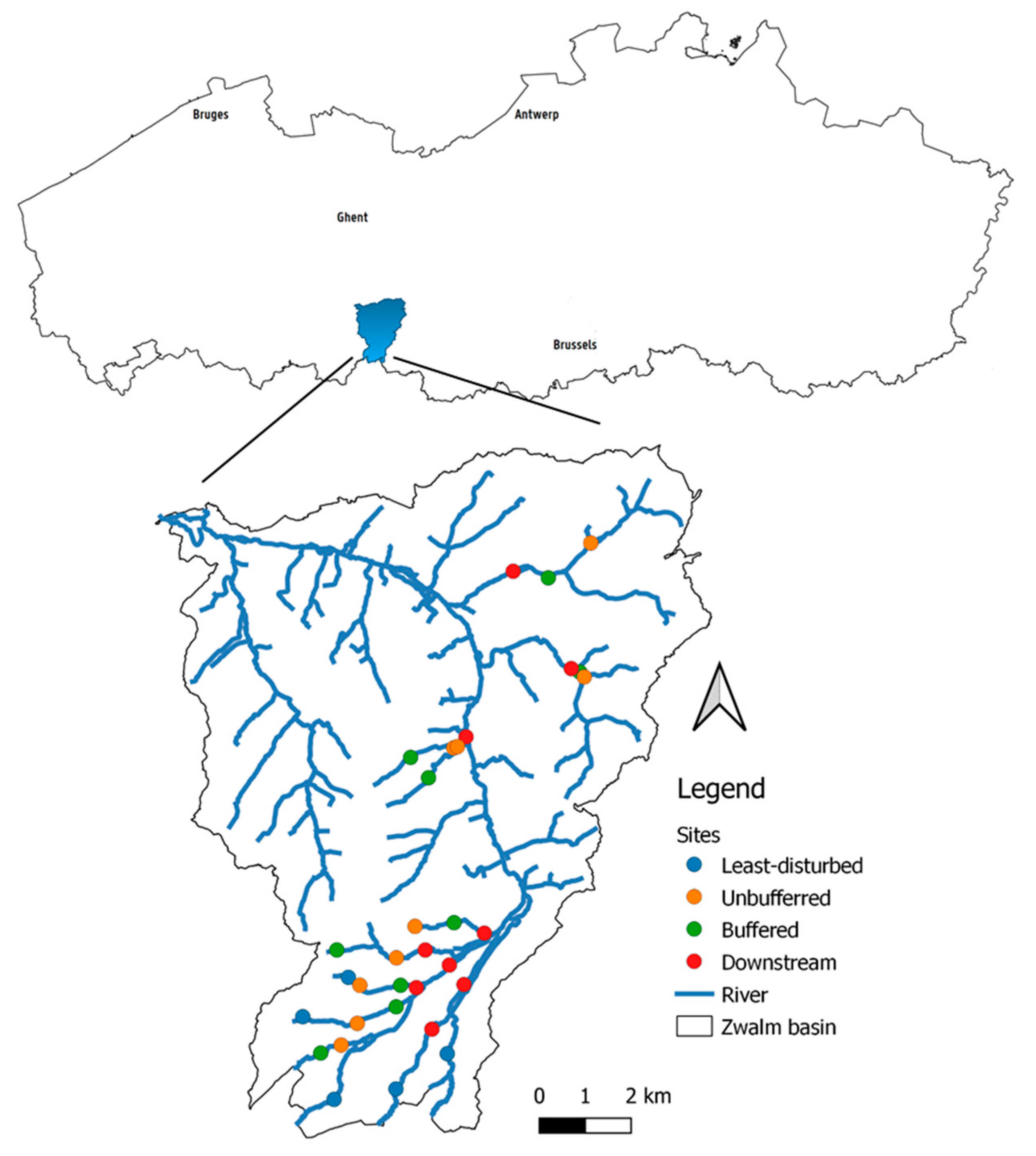
2.1. Study Area

The Zwalm river basin is situated in the south-western part of Flanders (Belgium), has a total catchment area of 117 km² (Figure 1) [55] and is dominated by sandy loam [56]. Annual rainfall ranges between 700 and 1000 mm [57]. Climatic conditions can be categorized as humid temperate [56,58]. Despite the Flanders region being generally flat, the topography of the basin is best described as rolling hills, mild slopes and altitudinal differences of up to 150 m [56,59]. These attributes have strong amenity values and offer opportunities for recreation and tourism. The land use within the basin is mainly agriculture (arable crops and pasture) with about 10% urban land cover [56,59]. The Zwalm river forms the main stem of the catchment and has a length of 22 km before flowing into the larger river Scheldt [57,60]. At the confluence, the Zwalm river has an average discharge of about 1 m³ s⁻¹ with a very irregular regime (i.e., minimum and maximum flows ranging from below 0.3 m³ s⁻¹ during summer to 4.7 m³ s⁻¹ during the rainy periods) [55].

Despite the recognition of the Zwalm basin as a biodiverse region in Flanders, stream conditions within the basin are not without issues. For instance, soil erosion is one of the most significant processes which results in considerable transport of sediments throughout the river system [59]. The presence of a weir impedes migration of several organisms (e.g., eel). Many parts of the river are still contaminated by untreated urban wastewater and diffuse pollution from agricultural land [59].

2.2. Data Collection

2.2.1. Site Selection

This study was performed in the context of the ERA-NET BiodivERsA project CROSSLINK project (see Burdon et al. [46]) and employed the common CROSSLINK tiered sampling design. Firstly, the paired approach focused on the immediate local implications of the presence of woody riparian vegetation. We sampled 12 streams flowing through an impacted (predominantly agricultural) landscape and 9 of those streams had two paired sites: an upstream site with no riparian buffer and a downstream site with a riparian buffer (i.e., leading 18 sites in total). Secondly, the network approach testing aspects of longitudinal connectivity involved 14 additional sites distributed throughout the river network (e.g., upstream and downstream of the site pairs). Within these sites, two site types are included: least-disturbed headwater reference sites and more degraded downstream matrix sites. The latter sites show the potential cumulative impacts of catchment land uses. There were, however, exceptions to this design in the Zwalm River basin case study. The majority of woody riparian buffers in the Zwalm River network were located at the headwaters of streams. This means that either the stream source was located within the woody riparian buffer or the upstream unbuffered reach only had intermittent flows and thus violated the site selection criteria (cf. Burdon et al. [46]). Hence, additional downstream matrix sites were used as surrogates for the unbuffered reach in four site pairs. In the Zwalm basin, there were five least-disturbed sites (Lds), nine paired sites (buffered (Bf) and unbuffered (Ubf) sites) and nine downstream matrix sites (Lon).

2.2.2. Riparian Characterisation

Three methods were used to characterize the riparian attributes of each study site: a quick assessment method resulting in a qualitative index, quantitative assessment focused on measuring a variety of riparian attributes in six plots (10 × 5 m) and quantification based on GIS data. Detailed information on the quick and quantitative riparian assessment are presented in Burdon et al. [46]. Both surveys were carried out in late spring of 2018 from 22 May to 18 June, when leaf-out was complete for all tree/shrub species and targeted both banks. A summary of the different riparian attributes is presented in Table S1.

Quick Assessment—Riparian condition was surveyed by using an assessment of 13 qualitative attributes, including shading of water, buffer width, buffer intactness, vegetation component of buffer and adjacent land, bank stability, livestock access, riparian soil denitrification potential, land slope, groundcover of buffer and/or adjacent land, soil drainage and rills/channel. This assessment follows the protocol described by Harding et al. [61], which was adapted to European conditions (Table S2). Attributes were graded from poor (1) to excellent (5) on each bank over the habitat assessment reach (50 m). Subsequently, at each study site, bank scores were averaged to provide a single value for riparian condition.

Quantitative assessment—Riparian habitat characteristics were surveyed in the riparian zones adjacent to the habitat assessment reach (50 m) at each study site. Six 50-m² rectangular plots (10 m × 5 m) were used to describe vegetation characteristics. These plots were located close to the stream edge, did not overlap and spread across the habitat assessment reach, capturing the full heterogeneity present at the study sites (Figure S1). For each plot, the pooled cover (% area) of different vegetation/habitat categories was estimated: managed short grasses (e.g., grazed or mown); unmanaged grasses and long grasses, including rushes and sedges; herbs and herbaceous vegetation, including forbs; mosses and lichens growing on the ground; small trees and shrubs (diameter at breast height (DBH) <5 cm); rocks and bedrock; bare ground; plant litter including leaves; other (e.g., roads, fences and embankments). The cover of each category was estimated as a vertical projection on to a horizontal plane (i.e., the ground). If plants in one category occurred in multiple layers then only the vertical projection on the ground was considered. Furthermore, the trees with DBH ≥5 cm and their circumference at breast height (~130 cm) were identified and measured in each plot. Trees were identified to the species level using a local identification guide [62]. Canopy cover was also measured at zenith from the center of each plot (Figure S1) using the smartphone app “CanopyApp” (University of New Hampshire, Durham, NH, USA). Measurements in each plot were averaged to provide a single value of riparian attributes in each site. Moreover, tree richness and abundance were calculated, which are the total number and count of tree species per site, respectively.

Quantification based on GIS data—Riparian characterization of each site was also obtained from GIS data using different spatial units. Four spatial units were used: Loc300mUP, which is the polygon 300 m upstream of the sampling sites (i.e., the recorded coordinates) with 50-m width on each stream bank, Loc200mUP which is the polygon 67 and 133 m downstream and upstream, respectively, of the sampling sites (resulting in a total of 200 m length) with 25-m width on each stream bank, Loc100mUP which is the polygon 33 and 67 m downstream and upstream, respectively, of the sampling sites (resulting in a total of 100 m length) with 25-m width on each stream bank and RipCatch100, which is the whole riparian corridor upstream of the sampling sites with 50-m width on each side of the stream. The different riparian conditions quantified from GIS data are the land use, tree cover area and density, width of riparian woody vegetation patches and the average distance between riparian tree blocks upstream of a sampling site (

Table 1. The spatial units and the quantified riparian attributes considered in this study. Quantified attributes are indicated with x.

Spatial Units	Loc100mUP, Units	Loc200mUP, Units	Loc300mUP, Units	RipCatch100, Units	GIS Source
Land use
Agricultural, forest and shrub Pasture and grassland Urban and industrial	x, m2	x, m2	x, %	x, %	BKK
Wetland and waterbodies			x, %	x, %	BKK
Tree cover
Tree cover area			x, %	x, %	Copernicus
Tree cover density			x, %	x, %	Copernicus
Width of each riparian land use (agricultural, forest, pasture and urban)
Min. width	x, m	x, m	x, m		BKK
Mean width	x, m	x, m	x, m		BKK
Distance between all riparian forest blocks upstream of a sampling site
Distance between 100 m forest blocks				x, m	BKK
Distance between 50 m forest blocks				x, m	BKK
Distance between 25 m forest blocks				x, m	BKK

Note: BKK is a 1-m resolution land cover dataset obtained in 2015 [63]. Copernicus is a 20-m resolution land cover dataset [64].

).

2.2.3. Other Environmental Variables

For each site, a set of environmental variables was quantified in addition to the riparian characteristics: catchment size, total inorganic nitrogen (ammonium-, nitrite- and nitrate-nitrogen), total phosphorus, biological oxygen demand, water pH, dissolved oxygen saturation, conductivity, water temperature, average stream width and percentage of fine sediments. The catchment size was calculated using the 5-m resolution Digital Elevation Model (DEM) [65]. Water samples were collected during the autumn of 2017 and analyzed for total inorganic nitrogen, total phosphorus and biological oxygen demand following a standard method [66]. In situ measurements were performed for pH, dissolved oxygen saturation, water temperature and specific conductivity of water using the YSI probes (YSI 6600 V2 and YSI 6600 V1, Yellow Springs, OH, USA) and WTW probe (Three-Multi 3430 IDS, WTW GmbH, Weilheim, Germany). Cross-sectional measurements of stream width were recorded in 5–6 transects that were distributed in a stratified random approach throughout the 50-m reach. “Wolman walk” methodology [67] was performed to determine the percentage of fine sediments (silt and clay). For details, we refer to Burdon et al. [46].

2.3. Invertebrate Collection

Riparian invertebrates consumers—We collected two groups of invertebrates commonly found in riparian zones that are known to predate on aquatic macroinvertebrates: arachnids (web-building and free-living spiders) and ground beetles (carabid) [68]. Sampling occurred in dry weather conditions during the spring between 22 May and 19 June, 2018. The sampling method used a semi-quantitative approach involving visual searches and collection by a hand net to obtain a relative indication of abundances (see Burdon et al. [46]). Both banks were surveyed over the habitat assessment reach using the same plots (i.e., 5 × 10 m = 50 m²) described above for riparian habitat quantitative assessment. The maximum total area searched was the plot area (i.e., 50 m²), but the area searched can be a fraction of 50 m² recorded from the plot boundaries. Whenever possible, 6 plots were searched. Five and ten minutes of sweep-netting and visual search were implemented by 1 and 2 persons, respectively. The searching of invertebrates was systematically started from the shoreline (i.e., near the water’s edge), with each collector following a transect parallel to stream edge moving further from the stream’s edge. Attempts were made to standardize the allocation of effort to reflect the proportion of different habitat types present. We calculated the “Catch per unit effort” (CPUE), which is a relative measure of abundance and richness allowing comparison between sites (Equation (1)). For details, we refer to the supporting information in Burdon et al. [46].

$$\mathrm{CPUE}=\frac{\mathrm{No}.\mathrm{of}\mathrm{invertebrates}}{\left(\mathrm{Total}\mathrm{area}\mathrm{sampled}.\mathrm{Duration}\mathrm{of}\mathrm{sampling}\right)}$$

(1)

Macroinvertebrates—Aquatic macroinvertebrates were sampled at each sampling site within a 30-m stretch of flowing water. The sampling area comprised the entire stream width along the predefined reach but efforts were made to ensure that sampling did not include areas that were dry in the recent past. We quantitatively sampled macroinvertebrates with a Surber sampler, which is a quadrant of 0.0625 m² (25 × 25 cm) to which a 500-µm mesh net is attached. A total of six replicate subsamples were collected in the sampling reach, i.e., three from erosional/riffle-run habitats and three from depositional/run-pool habitats. Sampling effort was standardized for 60 s, during which the bed substrate was disturbed to a maximum depth of 10 cm from the surface of the streambed. All subsamples were pooled together. The pooled macroinvertebrate sample was sieved (500-µm mesh) and sorted and then preserved in 10-mL tubes with 96% ethanol to reach a final concentration of 70%. Samples were identified under a stereomicroscope to the species level for Ephemeroptera, Plecoptera and Trichoptera (EPT) taxa and for several insects, gastropods and isopods, Hirudinea and Turbellaria family level for a few insects (i.e., Scirtidae, some Chironomidae, Tabanidae and Dytiscidae) and oligochaetes and genus level for the rest of the taxa using the taxonomic guides of Nilsson [69], Nilsson [70] and de Pauw and Vannevel [71].

2.4. Diversity Indices

We calculated a standard set of diversity metrics for each site: macroinvertebrate richness, which is the number of stream macroinvertebrate taxa per sample; macroinvertebrate abundance, which is the number of individual stream macroinvertebrates in a sample; Ephemeroptera, Plecoptera, Trichoptera (EPT) richness, which is the number of EPT taxa in a sample; EPT abundance, which is the number of individual EPT taxa in a sample; insect richness, which is the number of stream insect taxa in a sample; percent stream insect, which is the proportion of insects in a sample; No.1 in

Table 2. Equations of different indices, where $p_i$ is the proportion of individuals found of taxon $i$, $S$ is the total number of taxa and $N$ is the total number of individuals.

Indices	Equation	No.
% Insect	$\%Insect=\frac{Number of individual insects \times 100}{Total number of individual macroinvertebates}$	1
Shannon–Wiener index (H′)	$H^{\prime }=-{\displaystyle \sum _{i=1}^S}{p}_i\ln p_i$	2
Simpson’s index (D)	$D={\displaystyle \sum _{i=1}^S}{p}_i^2$	3
Pielou′s evenness index (J′)	$J^{\prime }=\frac{H^{\prime }}{\ln S}$	4
Margalef diversity index (d)	$d=\frac{S-1}{\ln N}$	5

. Diversity indices for stream macroinvertebrates were also determined for each site: the Shannon–Wiener index incorporates both richness and evenness components of biodiversity [72], No.2 in Table 2; the Simpson index is an index that gives more weight to common or dominant species [73], No.3 in Table 2; Pielou′s evenness index quantifies how numerically equal the community is [74], No.4 in Table 2; the Margalef diversity index (d) measures species richness [75], No.5 in Table 2. Lastly, metrics for terrestrial invertebrates (spider and carabids) were computed for each site: catch per unit effort (CPUE) in terms of abundance, which is the number of individual invertebrates per m² and per hour; CPUE in terms of richness, which is the number of invertebrates taxa per m² and per hour (see Equation (1)).

2.5. Data Analysis

2.5.1. Riparian Attributes and Diversity Metrics: Differences between Site Types

To visualize the differences in both riparian attribute data and biodiversity metrics among site types, boxplots of the site types were plotted as a function of the riparian attributes and invertebrate indices.

2.5.2. Relationships between Riparian Attributes and Diversity: Linear Regression Models

To relate each diversity metric (cf. Section 2.3) in response to each riparian attribute (Table S1), linear regression models (LM) were fitted. Linear regression models are widely applied and easy to implement and interpret [76,77]. It assumes linearity between dependent and independent variables. “Forward addition” was applied as a model selection procedure to determine whether the diversity metric was only associated with the riparian attribute or also related to the site type (i.e., least-disturbed sites, buffered and unbuffered sites and downstream sites)—i.e., first, the model was fitted with each riparian attribute; if it was significant at 5% level of significance, the “site type” was added in the model. The term “site type” entered the model as a nominal factor variable. All parameters in the linear regression were estimated using maximum likelihood [76]. To visualize the model, the results of the LM were visualized as the estimated mean of the diversity metric as a function of the selected riparian attribute.

Model assumptions were assessed by plotting the deviance residuals against fitted values to assess homogeneity and correctness of the mean model. All statistical tests were performed at the 5% level of significance. All analyses were performed with R software [78].

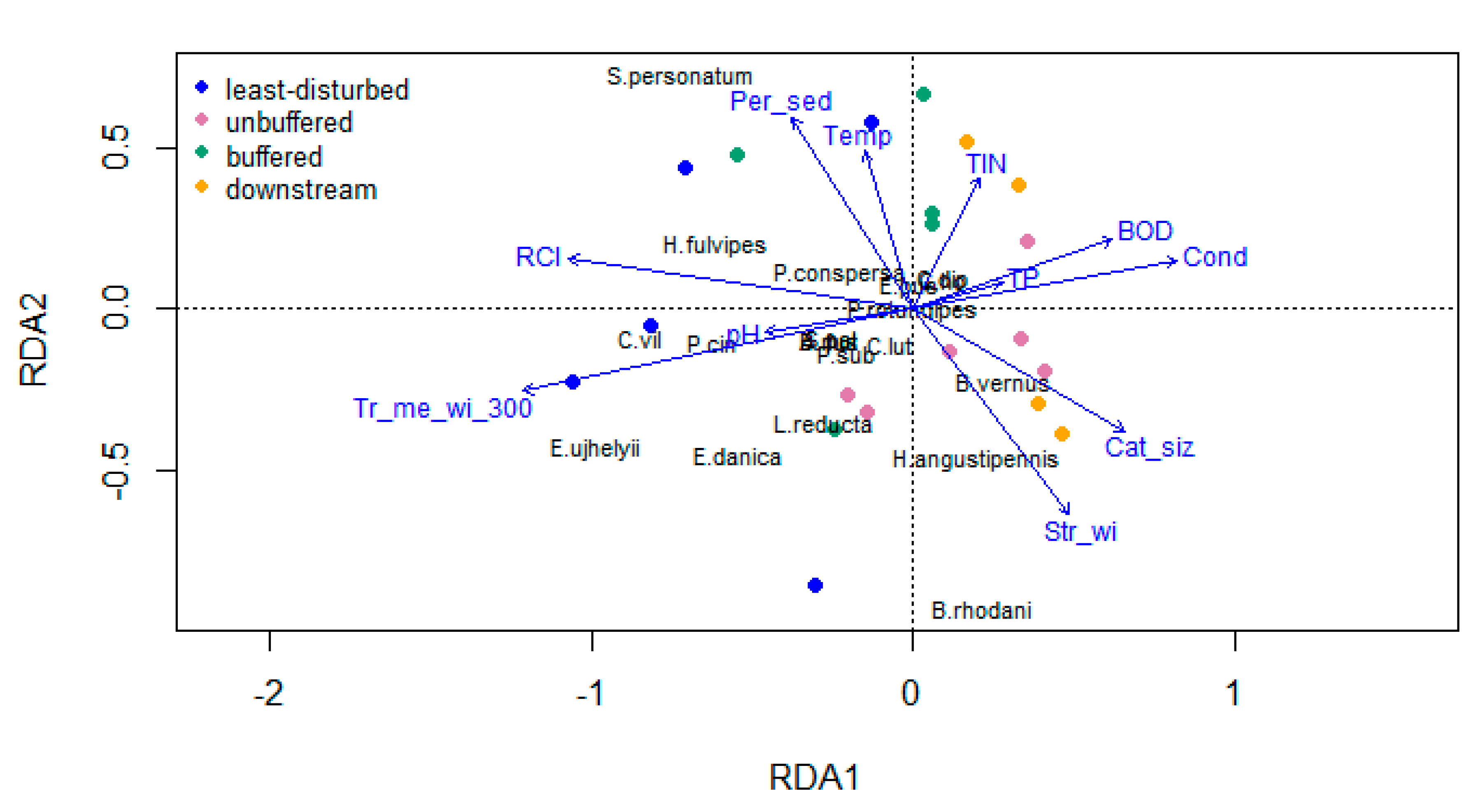
2.5.3. Redundancy Analysis

EPT taxa were associated with many riparian attributes and ordination analyses were used to (1) determine the riparian attribute that best explains the variability of EPT taxa occurrences and (2) explore the relationships between the occurrences of EPT taxa and the other environmental variables. We applied detrended correspondence analysis (DCA) to test whether a linear method or unimodal method was preferred. If the Length of Gradient (LoG) is higher than 3, a unimodal method is needed (i.e., canonical correspondence analysis), whereas if the LoG is smaller than 3, a linear method is designated (i.e., redundancy analysis (RDA)) [79]. As the LoG was lower than 3, RDA was implemented. RDA is a direct gradient analysis that accounts for multiple response variables and explanatory variables and attempts to effectively ordinate objects on axes that are built to maximize their relationship to the linear combinations of the explanatory variables [80]. All the other environmental variables and the riparian attributes that are statistically associated with EPT richness were initially included in the model. To reduce or eliminate multicollinearity in the model, we calculated the variance inflation factor (VIF) of each variable. Subsequently, the variable with the highest VIF was dropped. This process was repeated until the VIF of all variables was lower than 4 [81]. The analysis was performed using the vegan package [82] and R software [78].

3. Results

3.1. Riparian Characteristics

3.1.1. Implications of Spatial Resolution and Data Collection Methods

Riparian attributes varied among each other (Figure S2, Table S1). For instance, area of forest varied when quantified using GIS of the same spatial units but of different resolution (1-m and 20-m resolution) (Figure S2d,e). Between different spatial units, the percentage of forest area at least-disturbed sites was higher in the larger (RipCatch100m) than in smaller spatial unit (Loc300mUP) (Figure S2d–f). The coverage of trees was more pronounced in the least-disturbed sites and buffered sites in both the quick assessment and quantitative methods (Figure S2a–c,i) than in the GIS-based method (Figure S2d–h). The mean widths of forest and shrub in spatial units Loc200mUP and Loc300mUP were slightly different with respect to the site types (Figure S2g,h).

3.1.2. Differences among Site Types

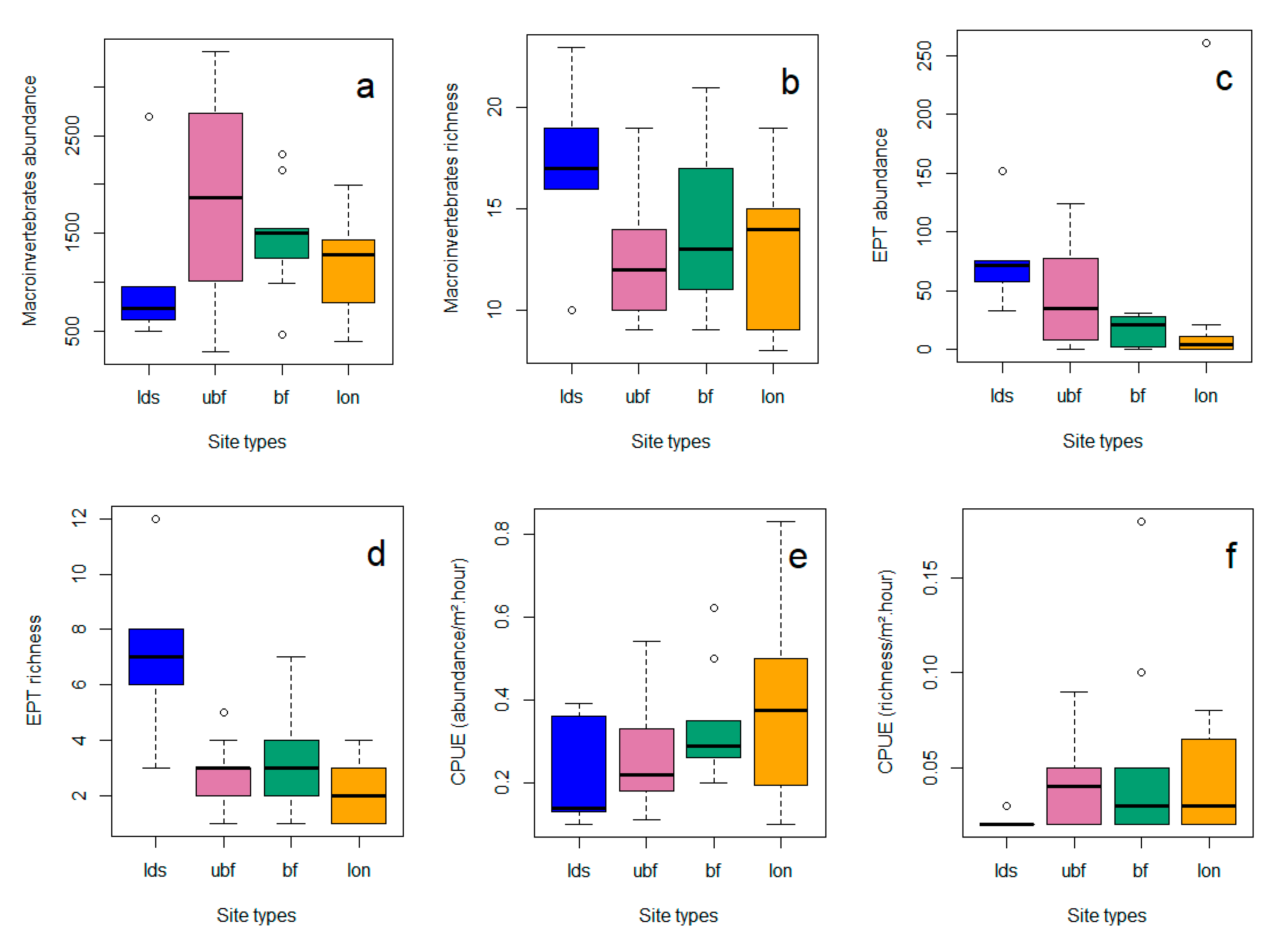
Riparian attributes also varied between site types (Figure S2). Buffer vegetation, percent tree coverage, tree abundance and tree richness differed among site types. These riparian attributes were quantified based on the quick assessment and quantitative methods. The percentages of forest area quantified from GIS data were generally higher at the least-disturbed sites than other site types (Figure S2d–f). The riparian forests were also generally wider in least-disturbed sites than other site types (Figure S2g,h) and most narrow at the downstream sites (Figure S2h). The median forest coverage of the whole riparian corridor upstream of a sampling site (RipCatch100m) was almost the same between the unbuffered, buffered and downstream site types due to their close spatial proximity and the general limited area of riparian forests in the catchment scale. It was also observed that both the least-disturbed sites and buffered sites were more diverse with riparian tree species (quantified by six plots of 50-m² area) compared to other site types.

3.2. Invertebrates

A total of 74 stream macroinvertebrate taxa and 45,495 individuals were found and identified in the Zwalm River basin during the spring of 2018 (Table S3). The number of individuals was lower in the least-disturbed sites compared to the unbuffered sites (Figure 2a). Many of the unbuffered sites were dominated by chironomids, gammarids and oligochaetes. On the other hand, stream macroinvertebrate taxa were the most diverse at the least-disturbed sites (Figure 2b). We found a total of 20 Ephemeroptera, Plecoptera and Trichoptera (EPT) taxa, totaling 1577 individuals. They were abundant in unbuffered and least-disturbed sites while they showed higher diversity in both buffered and least-disturbed sites (Figure 2c,d). Buffered sites had lower number of EPT taxa individuals than least-disturbed sites. EPT richness was also different between least-disturbed sites and downstream sites. The high abundance of EPT taxa in unbuffered sites was attributed to high densities of Baetis rhodani (Ephemeroptera: Baetidae) and Chaetopteryx villosa (Trichoptera: Limnephilidae). Concerning spiders and carabids, we found a total of 2303 individuals and 81 taxa, of which 31 taxa were carabids (Table S4). Both web building and free-living spiders were found. We found that diversity of our terrestrial invertebrate predator groups was lowest in least-disturbed sites, whereas abundance was greatest at downstream sites (Figure 2e,f). The most abundant taxa were Agelenidae, Araneidae, Linyphiidae and Theridiidae.

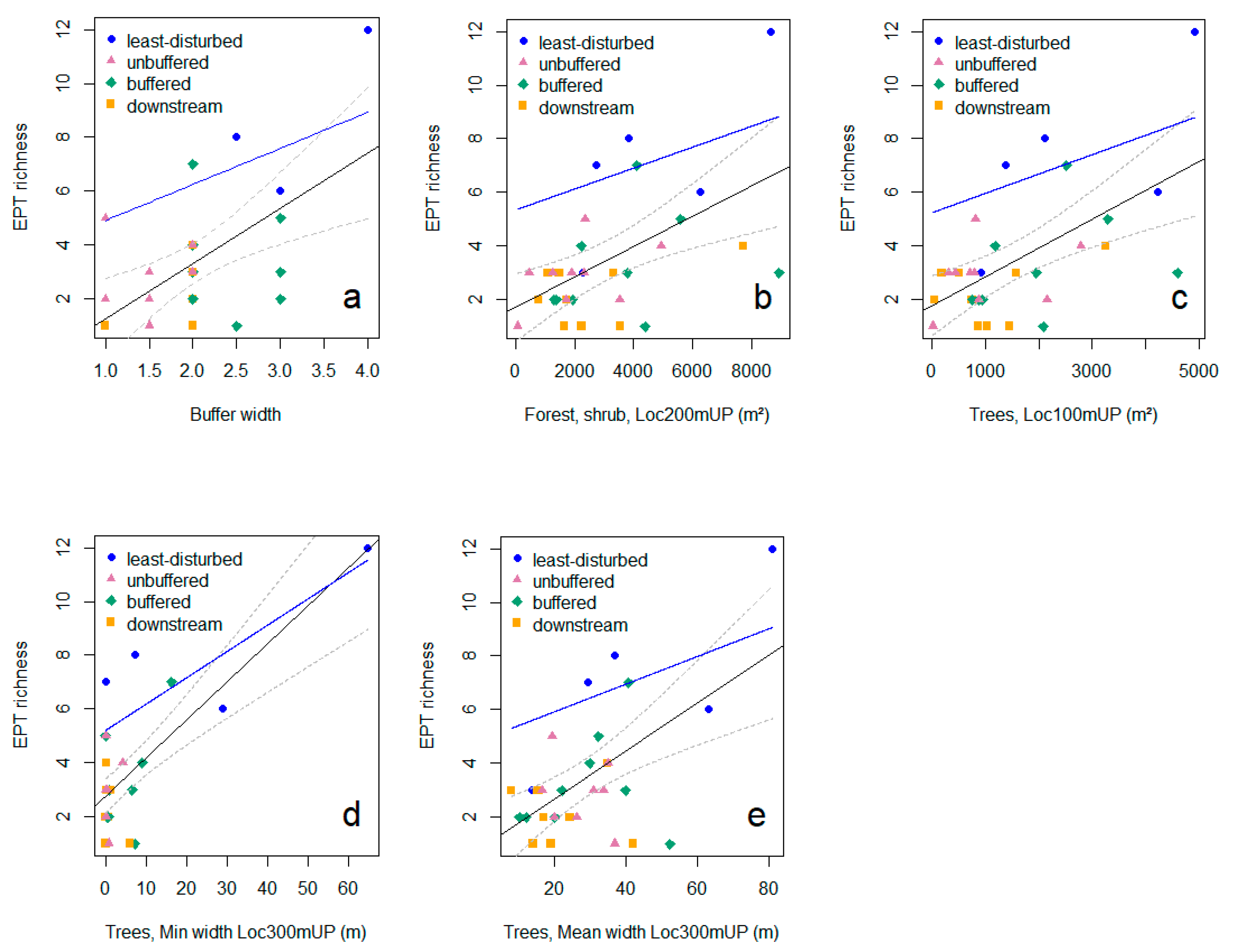
3.3. Relationships between Riparian Attributes and Invertebrate Diversity Metrics

Among the metrics, EPT richness showed the strongest responses and was mainly associated with riparian attributes obtained from quick assessment methods and GIS-based methods (

Table 3. Overview of associations between each riparian attribute and diversity metric obtained from the linear regression models. Only riparian attributes with significant associations are presented in the table. Black arrow represents statistically significant associations. Blue and red arrows indicate significant difference of site type—least-disturbed sites and unbuffered sites—from the other site types, respectively. Upward and downward arrows signify positive or negative associations, respectively. Graphical representations of selected models are presented in Figure 3 and Figure S3. The p-values are presented in Table S5.

Riparian Attributes	Abundance Inv 1	Richness Inv 1	Abundance EPT 2	Richness EPT 2	Richness Insects	% Insects	Shannon–Wiener	Margalef	Pielou’s Evenness Index	CPUE (Richness)
Quick Assessment
Adjacent groundcover				↑				↑
Buffer groundcover				↑				↑
Buffer width				↑↑
Soil drainage		↑		↑	↑			↑
Riparian Condition Index (RCI)				↑↑
Quantitative assessment
Unmanaged grass (%)						↑	↑		↑
Managed grass (%)										↑↓
Quantification based on GIS (spatial units)
Local riparian attributes
Forest 3, shrub (Loc100mUP) (m2)			↑↑	↑↑
Forest, shrub (Loc300mUP) (%)		↑		↑↑	↑			↑
Local riparian width attributes
Forest, shrub mean width (Loc100mUP)			↑	↑↑
Forest, shrub mean width (Loc300mUP)				↑↑	↑			↑
Forest, shrub min. width (Loc100mUP)				↑↑
Forest, shrub min. width (Loc300mUP)				↑↑	↑			↑
Full riparian corridor attributes
Forest, shrub (RipCatch100m)	↑			↑↑	↑			↑
Near distance to 25 m ForestBlocks (RipCatch100m)		↑

Note: ¹ Aquatic macroinvertebrates; ² Ephemeroptera, Plecoptera, Trichoptera; ³ forest refers to the woody riparian vegetation, such as trees and shrubs.

, Table S5). In general, EPT richness was positively related to the coverage of trees present in the riparian zone. Specifically, EPT richness increased with increasing buffer width and riparian condition index (RCI) and was higher at least-disturbed sites than other site types (Table 3, Figure 3a). EPT richness was, furthermore, positively associated with the forest area and width at 100–300 m upstream and full riparian corridor and was also higher in least-disturbed sites compared to other site types (Table 3, Figure 3b–e). At varying groundcover quality (for buffer and adjacent), EPT richness was higher at least-disturbed sites than other site types (Table 3). The Margalef index increased with increasing groundcover quality (Table 3, Figure S3a,b). The Margalef index was positively associated with the percentage of tree cover. Particularly, it was related to the larger spatial unit riparian data (Loc300mUp and RipCatch100m; Table 3, Figure S3c–f). The percentage of insects, the Shannon–Wiener index and Pielou’s evenness index increased with higher percentages of unmanaged grass (Table 3). Moreover, the Margalef index and invertebrate and insect richness rose with an increase in riparian soil permeability (in terms of soil drainage, Table 3). The richness-based metrics (i.e., invertebrate, EPT and insect richness and the Margalef index) were positively associated with the share of forest land use 300 m upstream of the sampling site. Richness of terrestrial invertebrate predators was only associated with the quantitative-based method, percent managed grass, wherein terrestrial invertebrates were more diverse if the percentage of managed grass increases. However, terrestrial invertebrate predators were less diverse in unbuffered sites than in the other site types.

The outcome of the redundancy analysis showed that mean width of the riparian forest at 300 m upstream of the sampling site (Tr_me_wi_300) had largest relative importance for the occurrence (presence-absence) of EPT communities (Figure 4). This was followed by the riparian quality index, RCI (Riparian Condition Index). The riparian attributes were, therefore, the most important variables for indicating the differences in EPT taxa occurrences. With regards to the environmental variables, conductivity and catchment size explained most of the variability. Conductivity, biological oxygen demand (BOD) and total inorganic nitrogen showed similar direction in the ordination space, an indication of a water pollution gradient. The occurrences of most EPT taxa were positively associated with the riparian attributes while they were negatively associated with conductivity, catchment size and biological oxygen demand. That is, the number of EPT taxa increased with increasing tree width and riparian quality while it decreased with increasing conductivity, catchment size and biological oxygen demand.

4. Discussion

4.1. Environmental Variables and Invertebrate Diversity

Our findings indicate that increases in woody forest vegetation in the riparian zones of our streams flowing through an otherwise heavily degraded landscape are associated with increases in the richness of freshwater macroinvertebrates, EPT richness and Margalef index. Specifically, the values of these metrics increase with increasing forest cover along the riparian zone at 300 m upstream of the sampling site. It has been reported that riparian vegetation enhances stream invertebrate diversity [44,45]. The findings of our study are particularly in line with the results of Rios and Bailey [83]. They observed an increase in EPT and invertebrate richness with increasing tree cover in the riparian zone at micro-basins. Similar to our study and catchment conditions, they also studied first- and second-order streams and mainly agricultural land cover, although some of their micro-basins are forest. The same patterns were observed by Death and Collier [84] in the Waikato (New Zealand) stream sites. This can be due to the various benefits of riparian forests: they help to stabilize the stream banks, minimize erosion or trap sediments, improve water quality through the reduction in nutrient runoff and enhance habitats for both fish and invertebrates [85]. Riparian forest also provides shade and maintains inputs of terrestrial leaf litter and wood [44,86,87]. The increased presence of EPT taxa in streams with more forested riparian vegetation might also reflect the provision of a suitable habitat for the terrestrial reproductive phase of these organisms [88] and is in line with previous observations indicating that greater exposure to wind and solar radiation is associated with reduced dispersal of adult aquatic insects [89]. Furthermore, aquatic insects leaving the water for emergence are particularly vulnerable to predation in open sand and gravel bars [90,91]. The presence of woody vegetation provides them shelter against predators. Forest riparian vegetation influences the riparian microclimate, which can play a role in conserving stream insects by maintaining cool temperatures and thereby improving riparian habitat quality for adult insects [87,92].

We also observed the dominance of certain taxa, such as chironomids and oligochaetes, in unbuffered sites. This observation is in line with the findings of Ivkovic et al. [93] and can be explained by the abundance of fine particulate organic matter, which is a food source of these organisms in unbuffered sites (open canopy) [93].

EPT richness and Margalef index also increased with increasing riparian forest width. Based on our findings, maximal diversity was observed at a mean riparian forest width of about 30–40 m for most site types except the least-disturbed sites (Figure 3e and Figure S2f). According to Castelle et al. [44], buffer widths of 3 to 200 m were found to be effective in protecting the biological integrity of streams, depending on site-specific conditions (e.g., the level of degradation in the stream, the value of streams and surrounding catchment land use); furthermore, a buffer width of at least 15 m is necessary to protect streams under most conditions. Another study, however, indicated the need for a 30-m riparian buffer width to positively affect species distribution and diversity [44]. This might be related to the mobility distance of some EPT taxa. Adult Trichoptera were found within 30 m of the stream edge in forested riparian zones [88]. A study has also shown that riparian forests as narrow as 5 m wide can considerably moderate air temperatures compared to treeless streams [94]. As lower air temperature increases the potential of adult Plecoptera to survive, riparian forest buffers may play a key role in the existence of these organisms, even if the riparian woody vegetation width is narrow [92].

Other environmental variables, such as catchment size, stream size and level of nutrient impact, are possibly confounded with variation in the spatial distribution of riparian attributes in our study, such as the extent of riparian cover upstream. However, such correlations are unlikely to have affected our analyses, given that these variables are not systematically correlated with the riparian attributes (Table S6). Moreover, the occurrence of EPT taxa is strongly related to the riparian attributes in comparison to other environmental variables (Figure 4). The RDA biplot indicates that most of the EPT taxa prefer lower nutrient concentrations and organic matter as well as smaller catchment sizes and stream widths. This is in line with previous findings that higher conductivity, BOD and nutrients are generally associated with lower abundance and/or diversity of EPT taxa [95,96]. Based on the linear regression models, EPT richness was higher at least-disturbed sites. The least-disturbed sites are characterized by limited or no domestic wastewater input. This suggests that the streams in the Zwalm river basin will significantly benefit from water quality improvements through the installation of wastewater treatment aside from the increase riparian forest cover.

Relationships between the terrestrial predator groups, carabid beetles and spiders, and riparian attributes were only detected when the quantitative assessment of riparian attributes was applied. This assessment method is the most localized method of quantifying riparian attributes. Studies suggest that both organisms are mainly affected by local factors [97,98,99]. Based on our findings, spider and carabid richness increased with an increasing percentage of managed grass but was lower at unbuffered sites than other site types. Unbuffered sites are locally characterized by no or very limited riparian forest compared to other site types (Figure S1a–c). Studies indicate that spider diversity increases with plant diversity [100] while carabids are more diverse in grassland and forest edge than forest interior [101]. The limited presence of riparian forest goes with low vegetation variability in unbuffered sites that most likely leads to lower carabid and spider richness. Our findings suggest the importance of both the grass vegetation as well as forests in riparian zones for the diversity of spiders and carabids.

Limitations of the study can be attributed to the temporal and seasonal variation of both environmental and biological variables [102,103]. Environmental variables most likely vary within the day and month, between seasons and within seasons. Biological samples also vary between and within seasons due to their inherent life cycle and responses to environmental changes. Although temporal deviations are not covered by our study, our study provides an indication of the role of woody riparian vegetation on invertebrate diversity and our samples were collected and processed in a standardized way.

4.2. Quantification of Riparian Attributes

Quantification of riparian habitats has been thoroughly presented in several previous studies which classified vegetation type according to height using LiDAR data in a reach length of 5–5.5 km and reach width of 5–15 m [41]. Juen et al. [43] examined the physical habitat of each stream within a channel length of 150 m using eleven 10² plots in each bank. Another study characterized riparian widths of 15–50 m at the watercourses within the subbasins [48]. Oldén et al. [47] estimated percentage cover of vegetation by eye estimation in 24 1-m² plots within the 15-m width from the stream. In our study, the quick assessment method (i.e., Riparian Condition Index) was assessed over 30 m on both banks, although the same length as the quantitative habitat assessment method encompassed a much wider coverage laterally from the stream channel (i.e., 30 m). The quick assessment method is subjective as it is assessed based on scores [46]. However, in our case study, only one person was evaluating the riparian attributes and therefore all the sites were estimated in the same way. For between-site comparisons, the findings of the study are, only to a lesser extent, affected by subjectivity. The quantitative method is the most localized riparian estimation method. It measures riparian attributes at 6 × 50-m² areas covering 30 m length in each bank. This method provides detailed information on riparian characteristics, such as percent canopy cover, unmanaged grass, managed grass, mosses, lichens, shrubs and plant litter, in addition to tree density and species composition. The quantification based on the GIS method covers a large spatial area due to the availability of basin-scale data. The accuracy may depend on the spatial resolution of the GIS data.

We found that the richness diversity indicators of aquatic macroinvertebrates were mainly associated with the riparian attributes quantified by the GIS-based and quick assessment methods while the terrestrial invertebrates (carabids and spiders) were associated with the quantitative assessment method. This suggests that the stream macroinvertebrates are affected at wider (about 25 to 50 m) and longer stretches (100 to 300 m) of riparian attributes while both carabids and spiders are mainly affected by localized habitat factors. Sponseller et al. [104] indicated that macroinvertebrate indices (e.g., EPT richness and Shannon–Wiener diversity index) were most closely related to land cover patterns evaluated at the 200-m sub-corridor scale (30-m width extending laterally). Their study suggests that local, streamside development effectively alters assemblage structure. Their findings are similar to our findings wherein a length of 100–300 m was related to the richness indices. Another study, however, reported that a 200-m reach of riparian woody vegetation did not affect the stream macroinvertebrates and EPT taxa richness [105] when compared with open reaches. However, their study focused on urban stream ecosystems while our catchment is dominantly agricultural landscape. The findings of our study provide insights into the spatial extent of riparian forest that needs to be evaluated and considered when relating invertebrate diversity.

4.3. Implications in Management and Future Studies

The findings of this study are relevant in the context of the EU Water Framework Directive (WFD) as one of its aims is to achieve a “good ecological status” for all waters [106]. Presently, there is no WFD intercalibrated indicator which is attributed to the riparian zones that relate to biological quality. Based on the findings of our study, wider width of tree forest can potentially increase the EPT taxa richness at a length of 300 m upstream of the target site. In particular, at least 30- to 40-m mean widths of riparian forest patches along the stream (e.g., 15 m of tree cover on each bank) can potentially deliver maximal EPT taxa richness (see Figure 3e and Figure 4). Despite the limited riparian forest within the Zwalm catchment, our findings illustrate their contribution to enhancing EPT taxa richness. To achieve good ecological status, patches of forest in the catchment can help but the whole catchment perspective is needed. Moreover, streams might benefit from the installation of a sewerage system and secondary wastewater treatment as our results show a significantly higher EPT richness at least-disturbed sites, characterized by no or limited untreated wastewater input (Figure 3). Approximately 40% of the basin’s inhabitants live in scattered population clusters and are therefore not connected to the centralized sewer system and nor is their wastewater treated [107], resulting in direct discharge to the streams. As most of the sampling sites are located in the headwaters, caution must be considered when findings are extrapolated in the main river of the catchment. Furthermore, the amount of riparian forest can be optimized to provide a balance between agricultural production and increasing the EPT taxa diversity. This can be implemented through an optimization framework in a future study (cf. Supplementary Information in Burdon et al. [46]) by integrating recent insights into the added value of buffer strips [108]. While stream invertebrates benefit from a catchment perspective, local actions could be sufficient for terrestrial consumers (i.e., carabids and spiders).

Future studies can be considered in determining the contribution of unmanaged grass on macroinvertebrate diversity at a catchment scale. Unmanaged grass at a large spatial scale was not explicitly analyzed in this study as the GIS data only provide grassland information and did not provide segregated data of managed and unmanaged grass. This information provides an added value in the context of riparian management within the Zwalm basin as some riparian zones are only covered with unmanaged grass.

5. Conclusions

Woody vegetation along the riparian zone is generally associated with the richness-related metrics of aquatic macroinvertebrates. Specifically, EPT richness shows a directly proportional relationship with riparian forest area and width, as exemplified in our case study area. Spiders and carabids were only associated with the riparian attributes quantified with the most localized method, suggesting that local riparian conditions mainly affect spiders and carabids while stream macroinvertebrates are affected by longer stretches (100–300 m) of riparian conditions. In particular, at least 30- to 40-m mean widths of riparian forest patches along the stream can potentially deliver the optimal EPT taxa richness. A GIS-based method is advised in quantifying riparian condition in order to investigate relationships with stream macroinvertebrate diversity as GIS data can cover a larger spatial coverage in comparison with the visual method of estimation. Our study shows that although local riparian habitat properties are important, broader spatial scales involving riparian forest cover still need to be evaluated and considered when assessing aquatic biodiversity and formulating river management strategies.

References

1. Grzybowski, M.; Glińska-Lewczuk, K. Principal threats to the conservation of freshwater habitats in the continental biogeographical region of central Europe. Biodivers. Conserv. 2019, 28, 4065–4097. [Google Scholar] [CrossRef] [Green Version]
2. Rodrigues, C.; Alves, P.; Bio, A.; Vieira, C.; Guimaraes, L.; Pinheiro, C.; Vieira, N. Assessing the ecological status of small mediterranean rivers using benthic macroinvertebrates and macrophytes as indicators. Environ. Monit. Assess. 2019, 191, 596. [Google Scholar] [CrossRef] [PubMed]
3. Aarts, B.G.W.; Van den Brink, F.W.B.; Nienhuis, P.H. Habitat loss as the main cause of the slow recovery of fish faunas of regulated large rivers in Europe: The transversal floodplain gradient. River Res. Appl. 2004, 20, 3–23. [Google Scholar] [CrossRef]
4. Grizzetti, B.; Pistocchi, A.; Liquete, C.; Udias, A.; Bouraoui, F.; van de Bund, W. Human pressures and ecological status of European rivers. Sci. Rep. 2017, 7, 205. [Google Scholar] [CrossRef] [Green Version]
5. Lytle, D.A.; Poff, N.L. Adaptation to natural flow regimes. Trends Ecol. Evol. 2004, 19, 94–100. [Google Scholar] [CrossRef] [PubMed]
6. Welcomme, R.L.; Winemiller, K.O.; Cowx, I.G. Fish environmental guilds as a tool for assessment of ecological condition of rivers. River Res. Appl. 2006, 22, 377–396. [Google Scholar] [CrossRef]
7. Forio, M.A.E.; Lock, K.; Radam, E.D.; Bande, M.; Asio, V.; Goethals, P. Assessment and analysis of ecological quality, macroinvertebrate communities and diversity in rivers of a multifunctional tropical island. Ecol. Indic. 2017, 77, 228–238. [Google Scholar] [CrossRef]
8. Poff, N.L.; Allan, J.D. Functional-organization of stream fish assemblages in relation to hydrological variability. Ecology 1995, 76, 606–627. [Google Scholar] [CrossRef]
9. Nguyen, T.; Forio, M.; Boets, P.; Lock, K.; Damanik Ambarita, M.; Suhareva, N.; Everaert, G.; Van der Heyden, C.; Dominguez-Granda, L.; Hoang, T.; et al. Threshold responses of macroinvertebrate communities to stream velocity in relation to hydropower dam: A case study from the Guayas river basin (Ecuador). Water 2018, 10, 1195. [Google Scholar] [CrossRef] [Green Version]
10. Bayramoglu, B.; Chakir, R.; Lungarska, A. Impacts of land use and climate change on freshwater ecosystems in france. Environ. Model. Assess. 2020, 25, 147–172. [Google Scholar] [CrossRef]
11. Deknock, A.; De Troyer, N.; Houbraken, M.; Dominguez-Granda, L.; Nolivos, I.; Van Echelpoel, W.; Forio, M.A.E.; Spanoghe, P.; Goethals, P. Distribution of agricultural pesticides in the freshwater environment of the Guayas river basin (Ecuador). Sci. Total Environ. 2019, 646, 996–1008. [Google Scholar] [CrossRef] [PubMed] [Green Version]
12. Cambien, N.; Gobeyn, S.; Nolivos, I.; Forio, M.A.E.; Arias-Hidalgo, M.; Dominguez-Granda, L.; Witing, F.; Volk, M.; Goethals, P.L.M. Using the soil and water assessment tool to simulate the pesticide dynamics in the data scarce Guayas river basin, Ecuador. Water 2020, 12, 696. [Google Scholar] [CrossRef] [Green Version]
13. Skoulikidis, N.T. The environmental state of rivers in the balkans-a review within the DPSIR framework. Sci. Total Environ. 2009, 407, 2501–2516. [Google Scholar] [CrossRef] [PubMed]
14. Haygarth, P.M.; Wood, F.L.; Heathwaite, A.L.; Butler, P.J. Phosphorus dynamics observed through increasing scales in a nested headwater-to-river channel study. Sci. Total Environ. 2005, 344, 83–106. [Google Scholar] [CrossRef]
15. Jiang, Y. China’s water scarcity. J. Environ. Manag. 2009, 90, 3185–3196. [Google Scholar] [CrossRef]
16. Hering, D.; Johnson, R.K.; Kramm, S.; Schmutz, S.; Szoszkiewicz, K.; Verdonschot, P.F.M. Assessment of european streams with diatoms, macrophytes, macroinvertebrates and fish: A comparative metric-based analysis of organism response to stress. Freshw. Biol. 2006, 51, 1757–1785. [Google Scholar] [CrossRef]
17. Mercado-Garcia, D.; Wyseure, G.; Goethals, P. Freshwater ecosystem services in mining regions: Modelling options for policy development support. Water 2018, 10, 531. [Google Scholar] [CrossRef] [Green Version]
18. Wang, Q.R.; Kim, D.; Dionysiou, D.D.; Sorial, G.A.; Timberlake, D. Sources and remediation for mercury contamination in aquatic systems - a literature review. Environ. Pollut. 2004, 131, 323–336. [Google Scholar] [CrossRef]
19. Clements, W.H.; Carlisle, D.M.; Lazorchak, J.M.; Johnson, P.C. Heavy metals structure benthic communities in colorado mountain streams. Ecol. Appl. 2000, 10, 626–638. [Google Scholar] [CrossRef]
20. Forio, M.A.E.; Villa-Cox, G.; Van Echelpoel, W.; Ryckebusch, H.; Lock, K.; Spanoghe, P.; Deknock, A.; De Troyer, N.; Nolivos-Alvarez, I.; Dominguez-Granda, L.; et al. Bayesian belief network models as trade-off tools of ecosystem services in the Guayas river basin in Ecuador. Ecosyst. Serv. 2020, 44, 101124. [Google Scholar] [CrossRef]
21. Wohl, E.; Angermeier, P.L.; Bledsoe, B.; Kondolf, G.M.; MacDonnell, L.; Merritt, D.M.; Palmer, M.A.; Poff, N.L.; Tarboton, D. River restoration. Water Resour. Res. 2005, 41, W10301. [Google Scholar] [CrossRef]
22. Edwards, A.M.C.; Freestone, R.J.; Crockett, C.P. River management in the humber catchment. Sci. Total Environ. 1997, 194, 235–246. [Google Scholar] [CrossRef]
23. Lock, K.; Asenova, M.; Goethals, P.L.M. Benthic macroinvertebrates as indicators of the water quality in Bulgaria: A case-study in the Iskar river basin. Limnol. Ecol. Manag. Inland Waters 2011, 41, 334–338. [Google Scholar] [CrossRef] [Green Version]
24. Okumah, M.; Chapman, J.P.; Martin-Ortega, J.; Novo, P. Mitigating agricultural diffuse pollution: Uncovering the evidence base of the awareness–behaviour–water quality pathway. Water 2019, 11, 29. [Google Scholar] [CrossRef] [Green Version]
25. Cole, L.J.; Stockan, J.; Helliwell, R. Managing riparian buffer strips to optimise ecosystem services: A review. Agric. Ecosyst. Environ. 2020, 296, 106891. [Google Scholar] [CrossRef]
26. Dosskey, M.G.; Vidon, P.; Gurwick, N.P.; Allan, C.J.; Duval, T.P.; Lowrance, R. The role of riparian vegetation in protecting and improving chemical water quality in streams1. Jawra J. Am. Water Resour. Assoc. 2010, 46, 261–277. [Google Scholar] [CrossRef]
27. Knight, K.W.; Schultz, R.C.; Mabry, C.M.; Isenhart, T.M. Ability of remnant riparian forests, with and without grass filters, to buffer concentrated surface runoff1. Jawra J. Am. Water Resour. Assoc. 2010, 46, 311–322. [Google Scholar] [CrossRef]
28. Dosskey, M.G. Toward quantifying water pollution abatement in response to installing buffers on crop land. Environ. Manag. 2001, 28, 577–598. [Google Scholar] [CrossRef]
29. Lowrance, R.; Altier, L.S.; Newbold, J.D.; Schnabel, R.R.; Groffman, P.M.; Denver, J.M.; Correll, D.L.; Gilliam, J.W.; Robinson, J.L.; Brinsfield, R.B.; et al. Water quality functions of riparian forest buffers in Chesapeake bay watersheds. Environ. Manag. 1997, 21, 687–712. [Google Scholar] [CrossRef]
30. Osborne, L.L.; Kovacic, D.A. Riparian vegetated buffer strips in water-quality restoration and stream management. Freshw. Biol. 1993, 29, 243–258. [Google Scholar] [CrossRef]
31. Raitif, J.; Plantegenest, M.; Roussel, J.-M. From stream to land: Ecosystem services provided by stream insects to agriculture. Agric. Ecosyst. Environ. 2019, 270–271, 32–40. [Google Scholar] [CrossRef] [Green Version]
32. Spooner, P.; Lunt, I.; Robinson, W. Is fencing enough? The short-term effects of stock exclusion in remnant grassy woodlands in southern NSW. Ecol. Manag. Restor. 2002, 3, 117–126. [Google Scholar] [CrossRef]
33. Maritz, B.; Alexander, G.J. Herpetofaunal utilisation of riparian buffer zones in an agricultural landscape near Mtunzini, South Africa. Afr. J. Herpetol. 2007, 56, 163–169. [Google Scholar] [CrossRef]
34. McCracken, D.I.; Cole, L.J.; Harrison, W.; Robertson, D. Improving the farmland biodiversity value of riparian buffer strips: Conflicts and compromises. J. Env. Qual. 2012, 41, 355–363. [Google Scholar] [CrossRef] [Green Version]
35. Gilbert, S.; Norrdahl, K.; Tuomisto, H.; Söderman, G.; Rinne, V.; Huusela-Veistola, E. Reverse influence of riparian buffer width on herbivorous and predatory Hemiptera. J. Appl. Entomol. 2015, 139, 539–552. [Google Scholar] [CrossRef]
36. Cole, L.J.; Brocklehurst, S.; Elston, D.A.; McCracken, D.I. Riparian field margins: Can they enhance the functional structure of ground beetle (Coleoptera: Carabidae) assemblages in intensively managed grassland landscapes? J. Appl. Ecol. 2012, 49, 1384–1395. [Google Scholar] [CrossRef]
37. Cole, L.J.; Brocklehurst, S.; Robertson, D.; Harrison, W.; McCracken, D.I. Riparian buffer strips: Their role in the conservation of insect pollinators in intensive grassland systems. Agric. Ecosyst. Environ. 2015, 211, 207–220. [Google Scholar] [CrossRef]
38. Gericke, A.; Nguyen, H.H.; Fischer, P.; Kail, J.; Venohr, M. Deriving a bayesian network to assess the retention efficacy of riparian buffer zones. Water 2020, 12, 617. [Google Scholar] [CrossRef] [Green Version]
39. Cole, L.J.; Brocklehurst, S.; McCracken, D.I.; Harrison, W.; Robertson, D. Riparian field margins: Their potential to enhance biodiversity in intensively managed grasslands. Insect Conserv. Divers. 2012, 5, 86–94. [Google Scholar] [CrossRef]
40. Parkyn, S.M.; Davies-Colley, R.J.; Halliday, N.J.; Costley, K.J.; Croker, G.F. Planted riparian buffer zones in New Zealand: Do they live up to expectations? Restor. Ecol. 2003, 11, 436–447. [Google Scholar] [CrossRef]
41. Grunblatt, J.; Meyer, B.E.; Wipfli, M.S. Invertebrate prey contributions to juvenile coho salmon diet from riparian habitats along three alaska streams: Implications for environmental change. J. Freshw. Ecol. 2019, 34, 617–631. [Google Scholar] [CrossRef] [Green Version]
42. Braun, B.M.; Pires, M.M.; Stenert, C.; Maltchik, L.; Kotzian, C.B. Effects of riparian vegetation width and substrate type on riffle beetle community structure. Entomol. Sci. 2018, 21, 66–75. [Google Scholar] [CrossRef]
43. Juen, L.; Cunha, E.J.; Carvalho, F.G.; Ferreira, M.C.; Begot, T.O.; Andrade, A.L.; Shimano, Y.; Leao, H.; Pompeu, P.S.; Montag, L.F.A. Effects of oil palm plantations on the habitat structure and biota of streams in eastern Amazon. River Res. Appl. 2016, 32, 2081–2094. [Google Scholar] [CrossRef]
44. Castelle, A.J.; Johnson, A.W.; Conolly, C. Wetland and stream buffer size requirements—A review. J. Environ. Qual. 1994, 23, 878–882. [Google Scholar] [CrossRef] [Green Version]
45. Urban, M.C.; Skelly, D.K.; Burchsted, D.; Price, W.; Lowry, S. Stream communities across a rural-urban landscape gradient. Divers. Distrib. 2006, 12, 337–350. [Google Scholar] [CrossRef]
46. Burdon, J.F.; Ramberg, E.; Sargac, J.; Forio, M.A.E.; de Saeyer, N.; Mutinova, T.P.; Moe, F.T.; Pavelescu, O.M.; Dinu, V.; Cazacu, C.; et al. Assessing the benefits of forested riparian zones: A qualitative index of riparian integrity is positively associated with ecological status in European streams. Water 2020, 12, 1178. [Google Scholar] [CrossRef] [Green Version]
47. Oldén, A.; Peura, M.; Saine, S.; Kotiaho, J.S.; Halme, P. The effect of buffer strip width and selective logging on riparian forest microclimate. For. Ecol. Manag. 2019, 453, 117623. [Google Scholar] [CrossRef]
48. Pissarra, T.C.T.; Valera, C.A.; Costa, R.C.A.; Siqueira, H.E.; Martins, M.V.; do Valle, R.F.; Fernandes, L.F.S.; Pacheco, F.A.L. A regression model of stream water quality based on interactions between landscape composition and riparian buffer width in small catchments. Water 2019, 11, 1757. [Google Scholar] [CrossRef] [Green Version]
49. Lock, K.; Goethals, P.L.M. Predicting the occurrence of stoneflies (Plecoptera) on the basis of water characteristics, river morphology and land use. J. Hydroinform. 2014, 16, 812–821. [Google Scholar] [CrossRef]
50. Lock, K.; Goethals, P.L.M. Habitat suitability modelling for mayflies (Ephemeroptera) in Flanders (Belgium). Ecol. Inform. 2013, 17, 30–35. [Google Scholar] [CrossRef]
51. Lock, K.; Goethals, P.L.M. Distribution and ecology of the caddisflies (Trichoptera) of Flanders (Belgium). Ann. Limnol. Int. J. Limnol. 2012, 48, 31–37. [Google Scholar] [CrossRef]
52. Jacobus, L.M.; Macadam, C.R.; Sartori, M. Mayflies (Ephemeroptera) and their contributions to ecosystem services. Insects 2019, 10, 170. [Google Scholar] [CrossRef] [Green Version]
53. Morse, J.C.; Frandsen, P.B.; Graf, W.; Thomas, J.A. Diversity and ecosystem services of Trichoptera. Insects 2019, 10, 125. [Google Scholar] [CrossRef] [Green Version]
54. DeWalt, R.E.; Ower, G.D. Ecosystem services, global diversity, and rate of stonefly species descriptions (insecta: Plecoptera). Insects 2019, 10, 99. [Google Scholar] [CrossRef] [Green Version]
55. Dedecker, A.P.; Goethals, P.L.; De Pauw, N. Comparison of artificial neural network (ANN) model development methods for prediction of macroinvertebrate communities in the Zwalm river basin in Flanders, Belgium. TheScientificWorldJournal 2002, 2, 96–104. [Google Scholar] [CrossRef] [Green Version]
56. Pauwels, V.R.N.; Verhoest, N.E.C.; De Troch, F.P. A metahillslope model based on an analytical solution to a linearized boussinesq equation for temporally variable recharge rates. Water Resour. Res. 2002, 38, 31–33. [Google Scholar] [CrossRef]
57. Huygens, M.; Verhoeven, R.; De Sutter, R. Integrated river management of a small Flemish river catchment. Role Eros. Sediment. Transp. Nutr. Contam. Transf. Proc. 2000, 263, 191–199. [Google Scholar]
58. Troch, P.A.; De Troch, F.P.; Brutsaert, W. Effective water table depth to describe initial conditions prior to storm rainfall in humid regions. Water Resour. Res. 1993, 29, 427–434. [Google Scholar] [CrossRef]
59. Goethals, P.; Dedecker, A.; Gabriels, W.; de Pauw, N. Development and application of predictive river ecosystem models based on classification trees and artificial neural networks. In Ecological Informatics: Understanding Ecology By Biologically-Inspired Computation; Recknagel, F., Ed.; Springer: New York, NY, USA, 2003; pp. 91–107. [Google Scholar]
60. Dedecker, A.P.; Goethals, P.L.M.; D’Heygere, T.; Gevrey, M.; Lek, S.; De Pauw, N. Application of artificial neural network models to analyse the relationships between gammarus pulex l. (Crustacea, Amphipoda) and river characteristics. Environ. Monit. Assess. 2005, 111, 223–241. [Google Scholar] [CrossRef] [PubMed]
61. Harding, J.S.; Clapcott, J.; Quinn, J.; Hayes, J.; Joy, M.; Storey, R.; Greig, H.; Hay, J.; James, T.; Beech, M.; et al. Stream Habitat Assessment Protocols For Wadeable Rivers And Streams Of New Zealand; School of Biological Sciences, University of Canterbury: Christchurch, New Zealand, 2009. [Google Scholar]
62. De Langhe, J.E.; Delvosalle, L.; Duvigneaud, J.; Lambinon, J.; Vanden Berghen, C. Flora Van België, Het Groot-Hertogdom Luxemburg, Noord-Frankrijk En De Aangrenzende Gebieden (Pteridofyten En Spermatofyten); Patrimonium van de Nationale Plantentuin van België, Meise: Meise, Belgium, 1988; p. 972. [Google Scholar]
63. Agentschap Informatie Vlaanderen. Bodembedekkingskaart (BBK), 1 m Resolutie, Opname 2015; Vlaamse Overheid: Brussels, Belgium, 2019; Available online: http://www.geopunt.be/catalogus/datasetfolder/0230a22f-51c0-4aa5-bb5d-0d7eeeaf0ce8 (accessed on 1 October 2019).
64. European Union; Copernicus Land Monitoring Service 2018; European Economic Area (EEA). Copernicus Tree Cover Density 2015. European Commission Joint Research Centre (JRC). 2020. Available online: https://land.copernicus.eu/pan-european/high-resolution-layers/forests/tree-cover-density/status-maps/2015?tab=mapview (accessed on 2 October 2019).
65. Agentschap Informatie Vlaanderen. Digitaal Hoogtemodel Vlaanderen II, DTM, Raster, 5 m; Vlaamse Overheid: Brussels, Belgium, 2014; Available online: http://www.geopunt.be/catalogus/datasetfolder/9b0f82c7-57c4-463a-8918-432e41a66355 (accessed on 15 January 2019).
66. Forio, M.A.E.; Goethals, P.L.M. An integrated approach of multi-community monitoring and assessment of aquatic ecosystems to support sustainable development. Sustainability 2020, 12, 5603. [Google Scholar] [CrossRef]
67. Wentworth, C.K. A scale of grade and class terms for clastic sediments. J. Geol. 1922, 30, 377–392. [Google Scholar] [CrossRef]
68. Burdon, F.J.; Harding, J.S. The linkage between riparian predators and aquatic insects across a stream-resource spectrum. Freshw. Biol. 2008, 53, 330–346. [Google Scholar] [CrossRef]
69. Nilsson, A. Aquatic Insects Of North Europe. A Taxonomic Handbook. Vol. 1: Ephemeroptera, Plecoptera, Heteroptera, Neuroptera, Megaloptera, Coleoptera, Trichoptera, Lepidoptera; Apollo Books: Stenstrup, Denmark, 1996; p. 274. [Google Scholar]
70. Nilsson, A. Aquatic Insects Of North Europe. A Taxonomic Handbook. Vol. 2: Odonata, Diptera; Apollo Books: Stenstrup, Denmark, 1997; p. 440. [Google Scholar]
71. de Pauw, N.; Vannevel, R. Macro-Invertebraten En Waterkwaliteit. Determineersleutels Voor Zoetwatermacro-Invertebraten En Methoden Ter Bepaling Van De Waterkwaliteit; Stichting Leefmilieu: Antwerp, Belgium, 1991; p. 316. [Google Scholar]
72. Shannon, C.E.; Weaver, W. The Mathematical Theory Of Communication; University of Illinois Press: Urbana, IL, USA, 1949; p. 117. [Google Scholar]
73. Simpson, E.H. Measurement of diversity. Nature 1949, 163, 688. [Google Scholar] [CrossRef]
74. Pielou, E.C. The measurement of diversity in different types of biological collections. J. Theor. Biol. 1966, 13, 131–144. [Google Scholar] [CrossRef]
75. Margalef, R. Information theory in ecology. Int. J. Gen. Syst. 1958, 3, 36–71. [Google Scholar]
76. Zuur, A.F.; Ieno, E.N.; Walker, N.J.; Saveliev, A.A.; Smith, G.M. Mixed Effects Models And Extensions Ion Ecology With R; Springer Science & Business Media, LLC.: New York, NY, USA, 2009. [Google Scholar]
77. Dickman, P.W.; Sloggett, A.; Hills, M.; Hakulinen, T. Regression models for relative survival. Stat. Med. 2004, 23, 51–64. [Google Scholar] [CrossRef] [PubMed]
78. R Core Team. A Language and Environment for Statistical Computing; R Foundation for Statistical Computing: Vienna, Austria, 2016; Available online: https://www.R-project.org/ (accessed on 7 January 2019).
79. Ter Braak, C.J.F.; Prentice, C. A theory of gradient analysis. In Advances in Ecological Research Vol. 34; Caswell, H., Ed.; Elsiever Academic Press: Cambridge, MA, USA, 2004; pp. 266–282. [Google Scholar]
80. Buttigieg, P.L.; Ramette, A. A guide to statistical analysis in microbial ecology: A community-focused, living review of multivariate data analyses. FEMS Microbiol. Ecol. 2014, 90, 543–550. [Google Scholar] [CrossRef] [Green Version]
81. Hair, J.F.; Anderson, R.E.; Babin, B.J.; Black, W.C. Multivariate Data Analysis: A Global Perspective; Pearson Education, Inc.: Upper Saddle River, NJ, USA, 2010. [Google Scholar]
82. Jari Oksanen, F.; Blanchet, G.; Friendly, M.; Kindt, R.; Legendre, P.; McGlinn, D.; Minchin, P.R.; O’Hara, R.B.; Simpson, G.L.; Solymos, P.; et al. Vegan: Community Ecology Package. R Package Version 2.5-2. Available online: https://CRAN.R-project.org/package=vegan (accessed on 15 June 2020).
83. Rios, S.L.; Bailey, R.C. Relationship between riparian vegetation and stream benthic communities at three spatial scales. Hydrobiologia 2006, 553, 153–160. [Google Scholar] [CrossRef]
84. Death, R.G.; Collier, K.J. Measuring stream macroinvertebrate responses to gradients of vegetation cover: When is enough enough? Freshw. Biol. 2010, 55, 1447–1464. [Google Scholar] [CrossRef]
85. Vought, L.B.M.; Pinay, G.; Fuglsang, A.; Ruffinoni, C. Structure and function of buffer strips from a water-quality perspective in agricultural landscapes. Landsc. Urban. Plan. 1995, 31, 323–331. [Google Scholar] [CrossRef]
86. Clinnick, P.F. Buffer strip management in forest operations: A review. Aust. For. 1985, 48, 34–45. [Google Scholar] [CrossRef]
87. Quinn, J.M.; Boothroyd, I.K.G.; Smith, B.J. Riparian buffers mitigate effects of pine plantation logging on New Zealand streams: 2. Invertebrate communities. For. Ecol. Manag. 2004, 191, 129–146. [Google Scholar] [CrossRef]
88. Collier, K.J.; Smith, B.J. Dispersal of adult caddisflies (Trichoptera) into forests alongside three New Zealand streams. Hydrobiologia 1997, 361, 53–65. [Google Scholar] [CrossRef]
89. Carlson, P.E.; McKie, B.G.; Sandin, L.; Johnson, R.K. Strong land-use effects on the dispersal patterns of adult stream insects: Implications for transfers of aquatic subsidies to terrestrial consumers. Freshw. Biol. 2016, 61, 848–861. [Google Scholar] [CrossRef]
90. Hering, D.; Plachter, H. Riparian ground beetles (Coeloptera, Carabidae) preying on aquatic invertebrates: A feeding strategy in alpine floodplains. Oecologia 1997, 111, 261–270. [Google Scholar] [CrossRef]
91. Samways, M.J.; Barton, P.S.; Birkhofer, K.; Chichorro, F.; Deacon, C.; Fartmann, T.; Fukushima, C.S.; Gaigher, R.; Habel, J.C.; Hallmann, C.A.; et al. Solutions for humanity on how to conserve insects. Biol. Conserv. 2020, 242, 108427. [Google Scholar] [CrossRef]
92. Collier, K.J.; Smith, B.J. Interactions of adult stoneflies (Plecoptera) with riparian zones I. Effects of air temperature and humidity on longevity. Aquat. Insects 2000, 22, 275–284. [Google Scholar] [CrossRef]
93. Ivkovic, M.; Milisa, M.; Baranov, V.; Mihaljevic, Z. Environmental drivers of biotic traits and phenology patterns of Diptera assemblages in karst springs: The role of canopy uncovered. Limnologica 2015, 54, 44–57. [Google Scholar] [CrossRef]
94. Meleason, M.A.; Quinn, J.M. Influence of riparian buffer width on air temperature at whangapoua forest, coromandel peninsula, New Zealand. For. Ecol. Manag. 2004, 191, 365–371. [Google Scholar] [CrossRef]
95. Jerves-Cobo, R.; Everaert, G.; Iñiguez-Vela, X.; Córdova-Vela, G.; Díaz-Granda, C.; Cisneros, F.; Nopens, I.; Goethals, P. A methodology to model environmental preferences of EPT taxa in the Machangara river basin (Ecuador). Water 2017, 9, 195. [Google Scholar] [CrossRef] [Green Version]
96. Ab Hamid, S.; Md Rawi, C.S. Application of aquatic insects (ephemeroptera, plecoptera and trichoptera) in water quality assessment of Malaysian headwater. Trop. Life Sci. Res. 2017, 28, 143–162. [Google Scholar] [CrossRef] [PubMed]
97. Djoudi, E.; Marie, A.; Mangenot, A.; Puech, C.; Aviron, S.; Plantegenest, M.; Petillon, J. Farming system and landscape characteristics differentially affect two dominant taxa of predatory arthropods. Agric. Ecosyst. Environ. 2018, 259, 98–110. [Google Scholar] [CrossRef]
98. Li, X.; Liu, Y.H.; Duan, M.C.; Yu, Z.R.; Axmacher, J.C. Different response patterns of epigaeic spiders and carabid beetles to varying environmental conditions in fields and semi-natural habitats of an intensively cultivated agricultural landscape. Agric. Ecosyst. Environ. 2018, 264, 54–62. [Google Scholar] [CrossRef]
99. Schirmel, J.; Thiele, J.; Entling, M.H.; Buchholz, S. Trait composition and functional diversity of spiders and carabids in linear landscape elements. Agric. Ecosyst. Environ. 2016, 235, 318–328. [Google Scholar] [CrossRef]
100. Malumbres-Olarte, J.; Vink, C.J.; Ross, J.G.; Cruickshank, R.H.; Paterson, A.M. The role of habitat complexity on spider communities in native alpine grasslands of New Zealand. Insect Conserv. Divers. 2013, 6, 124–134. [Google Scholar] [CrossRef]
101. Magura, T.; Tóthmérész, B.; Molnár, T. Forest edge and diversity: Carabids along forest-grassland transects. Biodivers. Conserv. 2001, 10, 287–300. [Google Scholar] [CrossRef]
102. Van Echelpoel, W.; Forio, A.M.; Van der Heyden, C.; Bermúdez, R.; Ho, L.; Rosado Moncayo, M.A.; Parra Narea, N.R.; Dominguez Granda, E.L.; Sanchez, D.; Goethals, L.P. Spatial characteristics and temporal evolution of chemical and biological freshwater status as baseline assessment on the tropical island San Cristóbal (Galapagos, Ecuador). Water 2019, 11, 880. [Google Scholar] [CrossRef] [Green Version]
103. Jerves-Cobo, R.; Forio, M.A.E.; Lock, K.; Van Butsel, J.; Pauta, G.; Cisneros, F.; Nopens, I.; Goethals, P.L.M. Biological water quality in tropical rivers during dry and rainy seasons: A model-based analysis. Ecol. Indic. 2020, 108, 105769. [Google Scholar] [CrossRef]
104. Sponseller, R.A.; Benfield, E.F.; Valett, H.M. Relationships between land use, spatial scale and stream macroinvertebrate communities. Freshw. Biol. 2001, 46, 1409–1424. [Google Scholar] [CrossRef] [Green Version]
105. Roy, A.H.; Rosemond, A.D.; Paul, M.J.; Leigh, D.S.; Wallace, J.B. Stream macroinvertebrate response to catchment urbanisation (Georgia, USA). Freshw. Biol. 2003, 48, 329–346. [Google Scholar] [CrossRef]
106. European Commission. Directive 2000/60/ec of the European Parliament and of the Council of 23 October 2000 Establishing a Framework for Community Action in the Field of Water Policy. Available online: https://eur-lex.europa.eu/legal-content/EN/TXT/?uri=celex%3A32000L0060 (accessed on 22 October 2000).
107. Mouton, A.M.; Van der Most, H.; Jeuken, A.; Goethals, P.L.M.; De Pauw, N. Evaluation of river basin restoration options by the application of the water framework directive explorer in the Zwalm river basin (Flanders, Belgium). River Res. Appl. 2009, 25, 82–97. [Google Scholar] [CrossRef]
108. Stutter, M.; Kronvang, B.; Ó hUallacháin, D.; Rozemeijer, J. Current insights into the effectiveness of riparian management, attainment of multiple benefits, and potential technical enhancements. J. Environ. Qual. 2019, 48, 236–247. [Google Scholar] [CrossRef] [Green Version]
Figure 1. Locations of the sampling sites within the Zwalm River basin.
Water 12 03070 g001
Figure 2. Boxplots of stream macroinvertebrate abundance (a), stream macroinvertebrate richness (b), Ephemeroptera, Plecoptera and Trichoptera (EPT) abundance (c), EPT richness (d), catch per unit effort (CPUE)—terrestrial invertebrate abundance m−2 h−1 (e) and CPUE—terrestrial invertebrate richness m−2 h−1 (f), with respect to the site types lds (least-disturbed sites), ubf (unbuffered), bf (buffered) and lon (downstream).
Water 12 03070 g002
Figure 3. Mean EPT richness in relation to the quick assessment method, buffer width (a), and GIS methods, area of trees in spatial units Loc200mUP (b), Loc100mUP (c); minimum and mean width of trees in spatial unit Loc300mUP ((d,e), respectively) are represented by grey lines. Grey dash lines are the confidence interval and the dots represents the sampling points. The blue line represents the mean EPT richness in relation to the respective riparian attribute at least-disturbed site type. The p-values are presented in Table S5.
Water 12 03070 g003
Figure 4. Redundancy analysis (RDA) plots of Ephemeroptera, Plecoptera and Trichoptera (EPT) taxa in response to gradients of environmental variables’ riparian condition index (RCI), forest and shrub mean width at Loc300mUP (Tr_me_wi_300), water pH (pH), water temperature (Temp), percentage of fine sediments (Per_sed), conductivity (Cond), biological oxygen demand (BOD), catchment size (Cat_siz), stream width (Str_wi), total inorganic nitrogen (TIN) and total phosphorus (TP). Dots represent the sites. The EPT taxa are Agapetus fuscipes (A.fus), Baetis muticus (B.mut), Baetis rhodani (B.rhodani), Baetis vernus (B.vernus), Caenis horaria (C.ho), Centroptilum luteolum (C.lut), Chaetopteryx villosa (C.vil), Cloeon dipterum (C.dip), Electrogena ujhelyii (E.ujhelyii), Enoicyla pusilla (E.pus), Ephemera danica (E.danica), Hydropsyche angustipennis (H.angustipennis), Hydropsyche fulvipes (H.fulvipes), Lype reducta (L.reducta), Paraleptophlebia submarginata (P.sub), Plectrocnemia conspersa (P.conspersa), Potamophylax cingulatus (P.cin), Potamophylax rotundipes (P.rotundipes), Sericostoma personatum (S.personatum) and Silo pallipes (S.pal). The environmental variables explain 57.6% of variation in EPT taxa occurrences.
Water 12 03070 g004