Parameter Estimation and Uncertainty Analysis: A Comparison between Continuous and Event-Based Modeling of Streamflow Based on the Hydrological Simulation Program–Fortran (HSPF) Model

Abstract

Hydrologic modeling is usually applied to two scenarios: continuous and event-based modeling, between which hydrologists often neglect the significant differences in model application. In this study, a comparison-based procedure concerning parameter estimation and uncertainty analysis is presented based on the Hydrological Simulation Program–Fortran (HSPF) model. Calibrated parameters related to base flow and moisture distribution showed marked differences between the continuous and event-based modeling. Results of the regionalized sensitivity analysis identified event-dependent parameters and showed that gravity drainage and storage outflow were the primary runoff generation processes for both scenarios. The overall performance of the event-based simulation was better than that of the daily simulation for streamflow based on the generalized likelihood uncertainty estimation (GLUE). The GLUE analysis also indicated that the performance of the continuous model was limited by several extreme events and low flows. In the event-based scenario, the HSPF model performances decreased as the precipitation became intense in the event-based modeling. The structure error of the HSFP model was recognized at the initial phase of the rainfall-event period. This study presents a valuable opportunity to understand dominant controls in different hydrologic scenario and guide the application of the HSPF model.

1. Introduction

Hydrologic models have become a vital tool in dealing with many practical and challenging issues that arise in watershed management. Hydrologists usually apply hydrologic models to two scenarios: continuous modeling and event-based modeling [1,2,3,4,5,6,7]. Generally, event-based modeling considers an individual rainfall–runoff event in isolation, as opposed to continuous modeling, which simulates streamflow over a longer period [5]. Limited by data availability, precipitation and streamflow data are rarely collected at hourly or even finer scales for a long period. Therefore, continuous hydrologic models are usually applied at a daily timescale, while a sub-daily timescale is required for event hydrologic models [6,8]. Hydrologic processes and catchment responses to a single rainfall–runoff event at a finer-scale will be characterized by the event-based modeling. A continuous modeling contains integrated responses by synthesizing hydrologic processes over a broad scope of hydro-climatic conditions.

The consideration of both scenarios for parameter estimation can extensively catch the range of catchment responses, as well as provide key information in specific periods and events. Concurrently calibrating models for both scenarios requires considerable observed data; however, in practice, the available data are often insufficient in temporal resolution and duration. To bypass this obstacle, parameters calibrated in one scenario are directly used in the other scenario. The transfer of parameter values is based on the assumption that parameters in the two scenarios are interchangeable [9,10,11,12]. This is only partially true: some parameters (e.g., those related to topography) remain constant, whereas others depend on hydrologic patterns, especially precipitation. In general hydrologic modeling, various model components may lead to the dominance and interact with others over different scenarios, which highly complicates the task of parameter estimation. Some flow components dominate the continuous modeling, while they may be excluded to some extent for the case that underlying processes that are not active for the considered rainfall–runoff events. For example, in continuous modeling, evapotranspiration and subsurface flow are important components, but in event-based modeling, their dominance decreases [13]. As stated in Pfannerstill et al. [14], surface runoff generation is the most sensitive process during a rainfall–runoff event, while tile drainages are inactive in low flow periods. Values of parameters related to specific components may be transplanted between different scenarios in order to achieve a broadly satisfied modeling performance. However, a clear understanding of how the parameters vary among the scenarios is very helpful for parameter estimation, with the goal to reproduce the right results (i.e., the observed streamflow) for the right reasons [15]. Therefore, it is critical to discern controlling model components and to parameterize them adequately so they can function well.

Sensitivity analysis is a useful tool for assessing model behavior and identifying critical model components. A classical sensitivity analysis results in a parameter list ranked by their sensitivity indices over a continuous long-term period. In contrast, some time-varying analyses have detected the non-stationarity of parameter sensitivity, especially during the whole time series and selected parts such as rainfall–runoff events [14,16,17,18,19]. For example, as reported by Guse et al. [17], groundwater and evapotranspiration parameters are sensitive for the long continuous simulation where low flows dominate the majority of the period. Surface runoff and groundwater time delay parameters are closely linked with rainfall–runoff events. Srivastava et al. [20] studied a representative rainfall–runoff event and analyzed the parameter sensitivity with respect to surface-groundwater dynamics and peak flow. In Herman et al. [21], three rainfall–runoff events were selected to investigate parameter activation and results showed that parameter sensitivity emerges as a function of forcing patterns. It should be noted that previous work has only focused on a limited number and types of events, which may derive predictive biases. This study aims to apply the sensitivity analysis application to investigate the dynamic controls both in the continuous scenario and different rainfall–runoff events. Furthermore, predictive uncertainty derived from model parameters needs to be considered to enhance model interpretation [22,23]. A proper and detailed analysis of how the predictive uncertainty changes can help increase model reliability, although there are currently few examples of such comparisons under different scenarios and different types of rainfall–runoff events.

Distributed or semi-distributed hydrologic models has been extensively used for streamflow modeling, such as the Soil and Water Assessment Tool (SWAT), Storm Water Management Model (SWMM), Hydrological Simulation Program–Fortran (HSPF), Hydrologic Prediction for the Environment (HYPE), Mike SHE, and Hydrologic Modeling System (HEC-HMS) [24,25,26,27,28,29]. Recently, the HSPF models shows its promising ability in both continuous modeling [30,31,32,33] and event-based modeling [7,34,35,36]. However, to our knowledge, a clear understanding of how parameter estimation and predictive uncertainty related to the HSPF model vary between different scenarios and different event types has not been fully achieved. To this end, this study consists of: (1) applying the HPSF model for parameter estimation in both continuous modeling and event-based modeling; (2) comparing parameter sensitivity between the two scenarios; and (3) comparing the quantified predictive uncertainty in the aggregated full time period and different rainfall–runoff events.

2. Materials and Methods

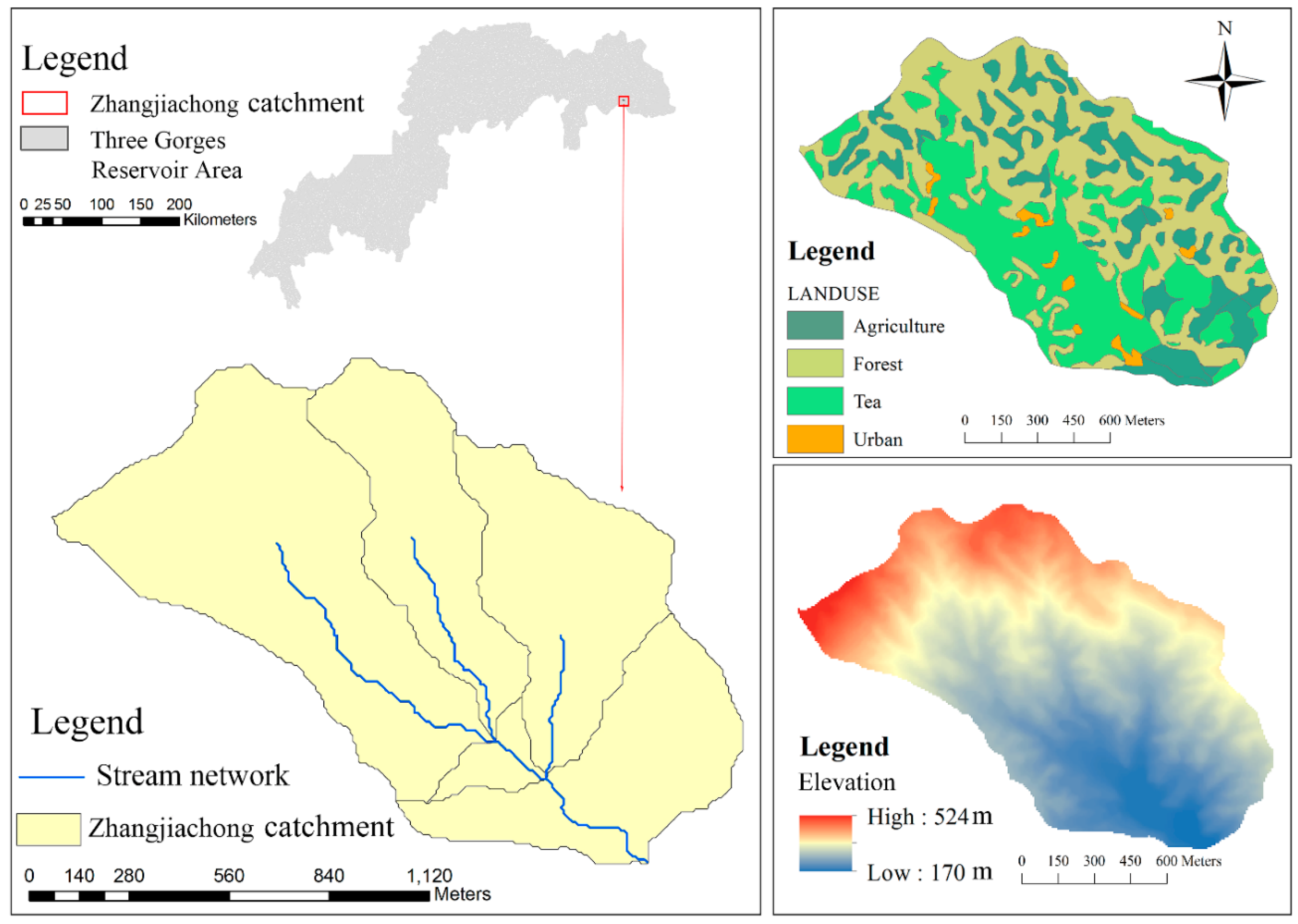
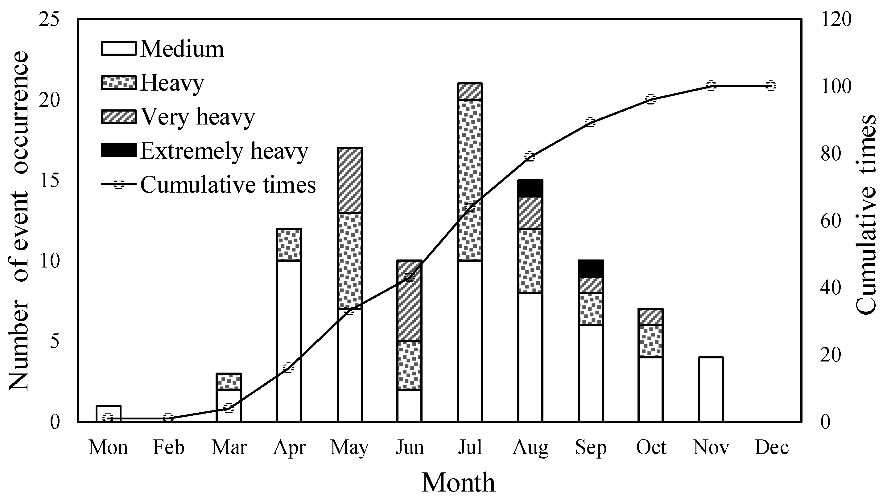
2.1. Study Site and Data Collection

The case study focuses on the Zhangjiachong catchment. It is in the upstream of the Three Gorges Reservoir (TGR) area, China. Figure 1 shows its location and spatial features. The total catchment area is approximately 162 ha. It is a typical small catchment in the TGR area because of its location, topography, climate, land use, and agricultural management. It is a sub-catchment of the Moping River catchment, which is a tributary to the Yangtze River. This catchment has hilly areas in the middle and upper part. The soil in the Zhangjiachong catchment is named as the yellow-brown type based on the China Soil Scientific Database. It is derived from granite or sandstone and is categorized as Alfisol in the soil taxonomy system of China. The yellow-brown soils are moderately leached, with a large soil bulk density and low porosity and permeability [37]. The land use is agriculture-dominated with local crops such as rape, corn, chestnut, and tea. Forest land occupies 42.9% of the total area. Only 2.1% is used as urban land. The mean annual air temperature and the annual precipitation are 18 °C and 1439 mm, respectively. The Zhangjiachong catchment is susceptible to severe soil erosion. As reported by the local water and soil conservation bureau, the soil erosion area caused by storm events had reached to 60% of the total area in 2001. The fertilizer amount is relatively high, especially on the tea lands, which accelerates plenty of nutrient losses into receiving waters.

Climate and underlying surface data are used to drive a HSPF running. Observed streamflows is required for calibration and validation. Data collection was conducted during 1 January 2010–31 December 2014. The contour map, soil map, and land use map were obtained from the local water and soil conservation bureau. Technical staff in the bureau developed the contour map at the scale of 1:10,000 on the basis of on-the-spot surveying and mapping. The land use map and soil map were plotted based on the contour map and field investigation. The digital elevation model (DEM) map with a grid size of 3 m × 3 m was generated from a conversion of the contour map. There is a rectangle shape-crested weir at the catchment outlet. A water level sensor continuously measured the water level at the outlet, and a data logger automatically recorded measurements every 15 min. A continuous time series of the climate data to drive the HSPF model was recorded by a weather station (MinMet auto weather station produced by Skye Instruments Ltd., Llandrindod Wells, UK) located at the gauging station near the catchment outlet.

The event separation method used in this study is based on previous research [38,39,40]. Two rainfall–runoff events were separated into two independent events if there was a continuous dry period of at least six hours. In this study, precipitation amount was used to classify rainfall–runoff events to be different types in previous research. This solution is computationally simple and straightforward but intended to facilitate streamflow forecasting and risk management [38,41,42,43,44]. The specific criterion is presented in

Table 1. Classification criteria of rainfall-runoff events.

Event Type	24-h Cumulative Amount	12-h Cumulative Amount
Light	0.1 mm–9.9 mm	0.1 mm–4.9 mm
Medium	10 mm–24.9 mm	5.0 mm–14.9 mm
Heavy	25.0 mm–49.9 mm	15.0 mm–29.9 mm
Very heavy	50.0 mm–99.9 mm	30.0 mm–69.9 mm
Extremely heavy	100 mm–249.9 mm	70.0 mm–139.9 mm
Torrential	≥250 mm	≥140 mm

. It should be mentioned that based on the monitoring experiences, the increased water level at the catchment outlet by light events was rarely more than 2 cm, which suggests that runoff generation was quite limited. Therefore, rainfall–runoff events of a light type (i.e., the accumulated rainfall amount was between 0.1 mm to 9.9 mm in 24 h or between 0.1 mm to 4.9 mm in 12 h) were excluded in this study. Torrential events did not occur so this type was also not considered. The other four event types, including medium, heavy, very heavy, and extremely heavy, were analyzed in this catchment. Their occurrence among different months are shown in Figure 2. Rainfall–runoff events in the Zhangjiachong catchment mainly occurred during April to October. The largest number of events were during July. The medium, heavy, and very heavy events happen most frequently in April, July, and June, respectively. Compared to other types of events, the number of extremely heavy events were rather small and they only took place in August and September. According to the analysis of the event characteristics, 12 rainfall events (

Table 2. Characteristics of the selected rainfall-runoff events.

Event	Start Date	Event Type	Rainfall Amount (mm)	Rainfall Duration (h)	Maximum Intensity (mm/h)
1	28 August 2013	Very heavy	56.5	3	40.5
2	21 April 2014	Medium	24.0	6	9.2
3	20 July 2014	Heavy	34.7	3	28.7
4	24 July 2014	Heavy	33.0	5	19.6
5	8 May 2014	Extremely heavy	104.7	10	45.4
6	9 February 2014	Heavy	48.2	8	10.0
8	25 June 2013	Heavy	31.6	6	30.3
11	24 September 2013	Heavy	48.1	20	4.4
7	15 April 2014	Medium	18.2	2	14.6
9	25 June 2014	Heavy	37.4	11	7.9
10	7 August 2014	Very heavy	69.2	8	27.4
12	23 August 2014	Heavy	30.4	7	11.2

) were selected for the subsequent event-based modeling. The rainfall amount varied between 18.2 mm and 104.7 mm, covering event types from medium to extremely heavy. The event duration ranged from 2 h to 20 h. Short intense events were represented by 3-h duration with a maximum intensity of 40.5 mm/h, and long-lasting but very light events were represented by 20 h duration with a maximum intensity of only 4.4 mm/h. Among the 12 selected events, numbers 1 to 6 were chosen for calibration, and the rest was used for validation.

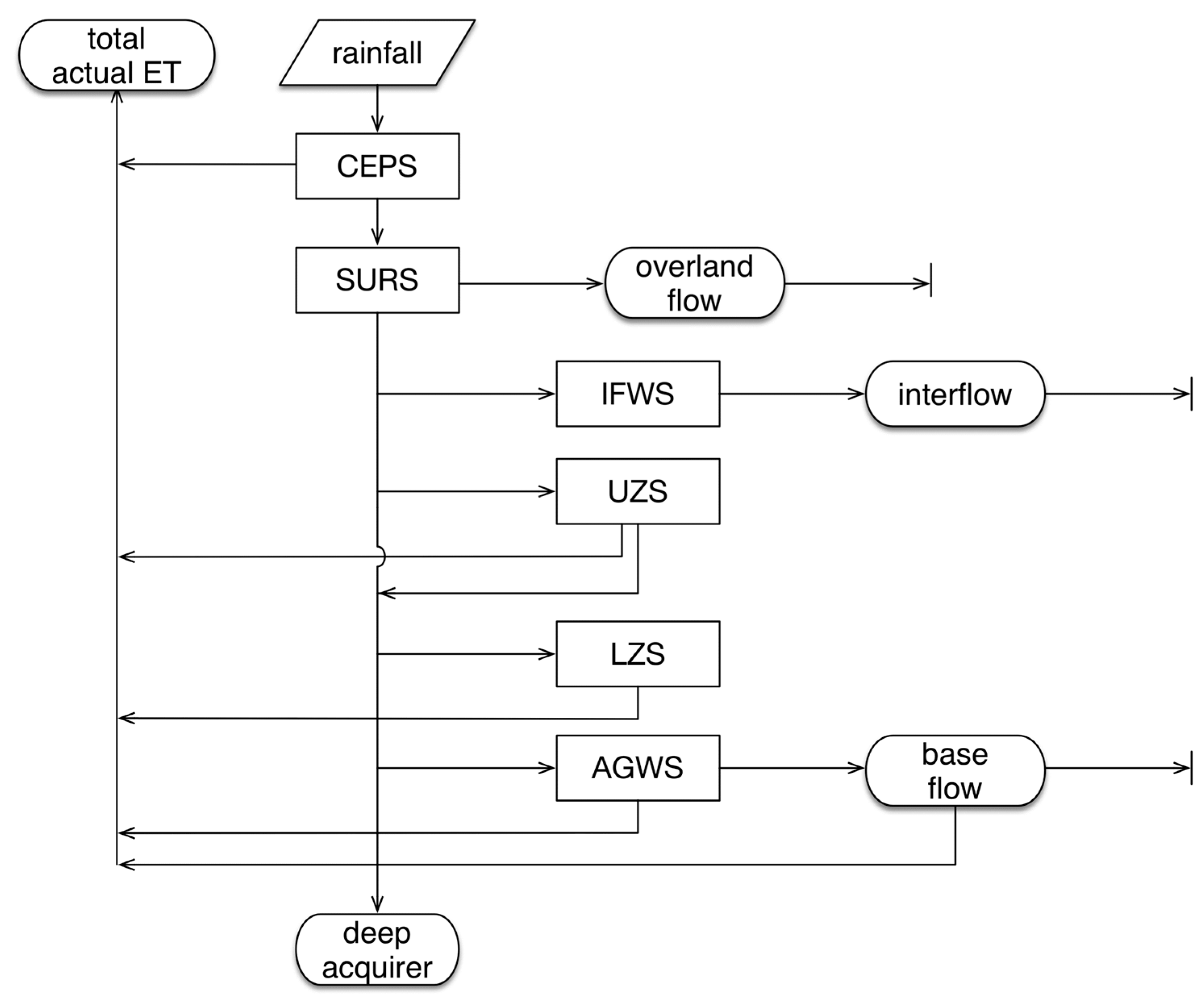
2.2. Description of the HSPF Model

The HSPF model is flexible enough to operate at time steps from 1 min to 1 h and to present output results daily and hourly. Importantly, both long-term (daily) hydrographs and event-based (hourly) hydrographs can be obtained. It divides a watershed into three modules: pervious land segment (PERLND), impervious land segment (IMPERLND), and reach segment (RCHRES). Fluxes and storages represent the movement and state of moistures. An outflow from a storage is typically calculated based on the current storage amount and the conceptual coefficients. Soil storages control the soil moisture rate and gravity drainage by infiltration and percolation. Evapotranspiration (ET) withdraws moistures from different storages. Part of the infiltration was directly drained into deep aquifers. Surface flow, interflow, and base flow contribute to the receiving water. A flow chart of water movement and storages represented in the PERLND module is presented in Figure 3. Key parameters for hydrologic modelling in the PERLND module were listed in

Table 3. Descriptions of the hydrologic parameters calibrated in the HSPF model.

Parameter	Description	Unit	Possible Range	Calibrated Values for Continuous	Calibrated Values for Event-Based
LZSN	Low zone nominal soil moisture storage	in.	2.0–15.0	5.502	3.703
INFILT	Index to mean soil infiltration rate	in./h	0.001–0.50	0.079	0.067
KVARY	Parameter to describe non-linear groundwater recession rate	in−1	0.0–5.0	3.643	0.202
AGWRC	Groundwater recession rate	day−1	0.85–0.999	0.987	0.850
DEEPFR	Fraction of infiltrating water which enters deep aquifers	none	0.0–0.50	0.005	0.057
BASETP	Fraction of potential evapotranspiration which fulfilled only as outflow exists	none	0.0–0.20	0.000	0.161
AGWETP	Fraction of remaining evapotranspiration that be met from active groundwater storage	none	0.0–0.20	0.000	0.166
CEPSC	Interception storage capacity	in.	0.01–0.40	0.010	0.123
UZSN	Nominal upper zone soil moisture storage	in.	0.05–2.0	0.668	0.415
INTFW	Interflow inflow parameter	none	1.0–10.0	1.000	9.999
IRC	Interflow recession parameter	day−1	0.3–0.85	0.300	0.300
LZETP	Index to lower zone evapotranspiration	none	0.1–0.9	0.400	0.494

. CEPSC controls the canopy interception; LZSN is the lower zone nominal storage; INFILT is the soil infiltration rate, while INTFW is the interflow coefficient. LZSN, INFILT, and INTFW are critical to determine gravity drainage of the moisture. UZSN is the upper zone nominal storage that controls the inflow to the upper zone and percolation amount. IRC is the recession coefficient of interflow, AGWRC and KVARY are two groundwater parameters used to calculate the amount of base flow, and DEEPFR is the fraction of the groundwater that enters the deep acquirer. BASETP, AGWETP, and LZETP are the three key parameters determining evapotranspiration. The RCHRES module assumes a water body as a single reach of an open or closed channel, or a completely mixed lake. The hydraulic processes of unidirectional flow will be simulated using this module. The geometric and hydraulic properties of a specific reach are summarized in a function table that facilitates in calculating flow routing [24]. Two essential files are required to run the HSPF model, that is the user control input (UCI) file and the watershed data management (WDM) file. The UCI file configures the parameter settings and module setup. The WDM file stores the time series of climate forcing and simulation results.

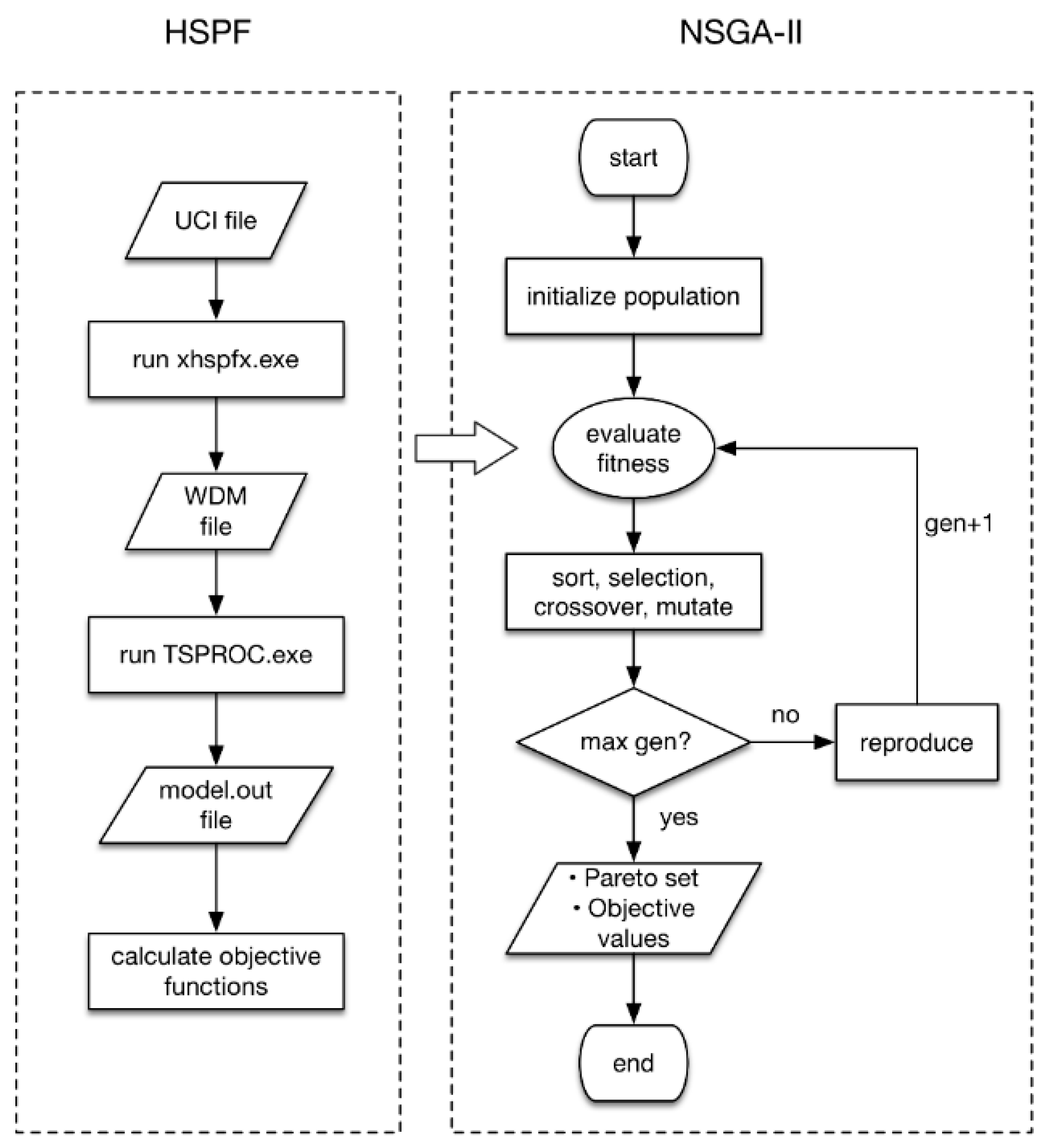
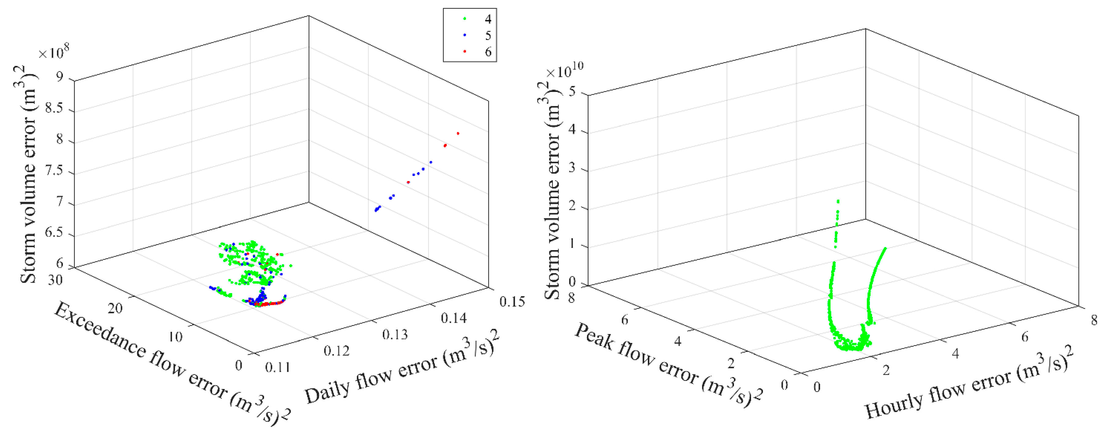
2.3. Multi-Objective Calibration

The non-dominated sorting genetic algorithm II (NSGA-II) was employed for the multi-objective calibration. The calibrated hydrologic parameters are showed in Table 3 with their descriptions. The NSGA-II is an efficient genetic algorithm (GA) that has been widely used in many disciplines with high performance [45]. It incorporates the non-dominated sorting and ranking selection with the crowded comparison operator into traditional GA. The Pareto front presents a trade-off surface consisting of a set of optimal solutions. This characteristic complies to the nature of multi-objective calibration. Figure 4 illustrates the procedure of the HSPF/NSGA-II calibration. TSPROC.exe processed the output time series of binary format into model.out file in text format, which facilitated the calculation of objective functions. The maximum generation number and initial population number were set as 2200 and 600, respectively, for the continuous modeling, and as 1200 and 600, respectively, for the event-based modeling.

The calibration period used for the continuous modeling was between 1 January 2011, and 31 December 2012, while validation was performed between 1 January 2013 and 31 December 2014. The spin up period for the continuous modeling was one-year (1 January 2010–31 December 2010) to stabilize the model from initial states to equilibrium. Three objective functions: squared error of daily flow (SEDF), squared error of different exceedance flow (SEEF), and squared error of volume in selected events (SEV), were calculated according to Equations (1)–(3). The selection of flow exceedances is an important part to calibrate the flow duration curves [1,46]. This study chose 10%, 50%, and 90% as the evaluation points, which referred to the methods used in Kim et al. [47] and Lumb and Kittle [48].

$$SEDF={{\displaystyle \sum }}_{i=1}^N{\left(Q_{sim,i}-Q_{obs,i}\right)}^2$$

(1)

$$SEEF={{\displaystyle \sum }}_{i=1}^{N_{10\%}}{\left(Q_{sim,10\%,i}-Q_{obs,10\%,i}\right)}^2+{{\displaystyle \sum }}_{i=1}^{N_{50\%}}{\left(Q_{sim,50\%,i}-Q_{obs,50\%,i}\right)}^2+ {{\displaystyle \sum }}_{i=1}^{N_{90\%}}{\left(Q_{sim,90\%,i}-Q_{obs,90\%,i}\right)}^2$$

(2)

$$SEV={{\displaystyle \sum }}_{i=1}^{N\_event}{\left(V_{sim,i}-V_{obs,i}\right)}^2$$

(3)

where Q is the daily flow; V is the volume of selected rainfall-runoff events; N is the number of daily time steps; sim represents simulated; obs represents observed; i is the time step index; N_event represents the number of selected events; and N_10%, N_50%, and N_90% represent the fractions of time that streamflow equals or exceeds specific flow rates.

As for the event-based modeling, multiple events were calibrated concurrently. The spin up period for each rainfall–runoff event was one month before the calibration. The three objective functions for multi-event calibration were averaged squared error of hourly flow rate (ASEHF), averaged squared error of volume (ASEV), and averaged squared error of peak flow (ASEPF), which were calculated as follows:

$$ASEHF=\left\{\begin{array}{c}{{\displaystyle \sum }}_{i=1}^{T_1}{\left({Q^{s_1}}_{sim,i}-{Q^{s_1}}_{obs,i}\right)}^2+{{\displaystyle \sum }}_{i=1}^{T_2}{\left({Q^{s_2}}_{sim,i}-{Q^{s_2}}_{obs,i}\right)}^2+\\ \dots +{{\displaystyle \sum }}_{i=1}^{T_n}{\left({Q^{s_i}}_{sim,i}-{Q^{s_i}}_{obs,i}\right)}^2\end{array}\right\}/n$$

(4)

$$ASEV={{\displaystyle \sum }}_{i=1}^n{\left(V_{sim,i}-V_{obs,i}\right)}^2/n$$

(5)

$$ASEPF={{\displaystyle \sum }}_{i=1}^n{\left(P_{sim,i}-P_{obs,i}\right)}^2/n$$

(6)

where $Q^{s_i}$ is the hourly flow in the ith event, T_n is the number of hourly time steps in event n, i is the time step index, n is the total number of calibrated events, V is the flow volume of an event, and P is the peak flow rate of an event. For each equation, the performance of a model simulation was assumed to be better when the objective function was closer to zero.

The statistical criteria for evaluating model performances in this study are HSPEXP method [48], Nash–Sutcliffe efficiency (NSE) [49], root mean squared error (RMSE), and coefficient of determination (R²), which are detailed in the Appendix A. For a better comparison of the parameter estimation between the two scenarios, the best overall performance (BOP) solution and optimized parameter range were both used. The BOP solution was selected by calculating and comparing the Euclidean distances between coordinate origin and Pareto solutions [50]. The optimized range for each parameter was determined as an NSE value more than 0.5.

2.4. Sensitivity and Uncertainty Analysis

All the hydrologic parameters in the calibration were investigated in terms of their sensitivity and uncertainty. Uniform distribution was selected for each parameter because there was no prior information regarding parameter distribution in this area. The prior parameter ranges are listed in Table 3. The sensitivity and uncertainty analysis were both based on 50,000 rounds of Monte Carlo (MC) simulations using the Latin hypercube sampling method.

2.4.1. Regional Sensitivity Analysis

The objectives for this section are to identify the dominant hydrologic parameters in the HSPF model and compare the controlling factors that lead to streamflow variability under the two different scenarios. Global sensitivity analysis (GSA) is usually recommended for non-linear and complex models because it considers the simultaneous variation of each parameter through the whole ranges [51]. Regionalized sensitivity analysis (RSA) was employed here to discern the controlling parameters and associated sub-processes that contribute most to the variability in streamflow. RSA was originally proposed by Spear and Hornberger [52]. Its implementation is based on Monte Carlo sampling on a whole distribution of parameter sets and is thus categorized as a GSA method. Typical steps needed to apply the RSA to hydrologic modeling can be summarized as follows: (1) define the distribution form of each selected parameter, (2) run models based on parameter groups derived from the MC samplings and evaluate each simulation using a goodness criterion, (3) classify the results into behavioral and non-behavioral groups according to a given threshold of the criterion, and (4) plot the relative cumulative probability distribution of the parameter in each group. An improved RSA was also proposed in which all parameter sets were ranked in terms of model performances and divided into 10 groups of equal size [53]. This method increases the information gained by the analysis. A sensitive parameter produces curves of different forms and separations, whereas the opposite indicates an insensitive parameter. This improved RSA method is used for the sensitivity analysis of the continuous and event-based scenarios. A MATLAB (version R2016a) toolbox called SAFE [54] was used to perform the RSA method in this study.

2.4.2. Generalized Likelihood Uncertainty Estimation

The generalized likelihood uncertainty estimation (GLUE) method was proposed by Beven and Binley [55]. Optimal value calibration is the classical calibration method. On the contrary, GLUE focuses on equifinality, that is, multiple parameter sets can produce the same or very similar model results. Because GLUE is conceptually simple and easy to implement, it is commonly used in the field of streamflow modeling. The typical steps for implementing GLUE can be summarized as follows: (1) define the priori probability distribution and value range for each parameter, and define the likelihood measure that indicates the model performance of a particular parameter set; (2) perform MC simulations and calculate the likelihood measure for each parameter set; (3) classify the parameter groups as behavioral and non-behavioral groups based on a pre-defined threshold and assign a likelihood weight to each behavioral parameter set; and (4) develop the cumulative distribution function (CDF) using the behavioral models, and then construct confidence intervals. NSE was selected as the likelihood measure and the threshold was selected to be 0.5. Two indicators were used to evaluate the predictive uncertainty: (1) the p-factor, the percentage of observations bracketed by the 95% prediction uncertainty (95 PPU) bounds, and (2) the r-factor, the average thickness of the 95 PPU bounds divided by the standard deviation of the observations. A reliable prediction is indicated by a p-factor close to 100% and a r-factor close to 1 [56].

3. Results and Discussion

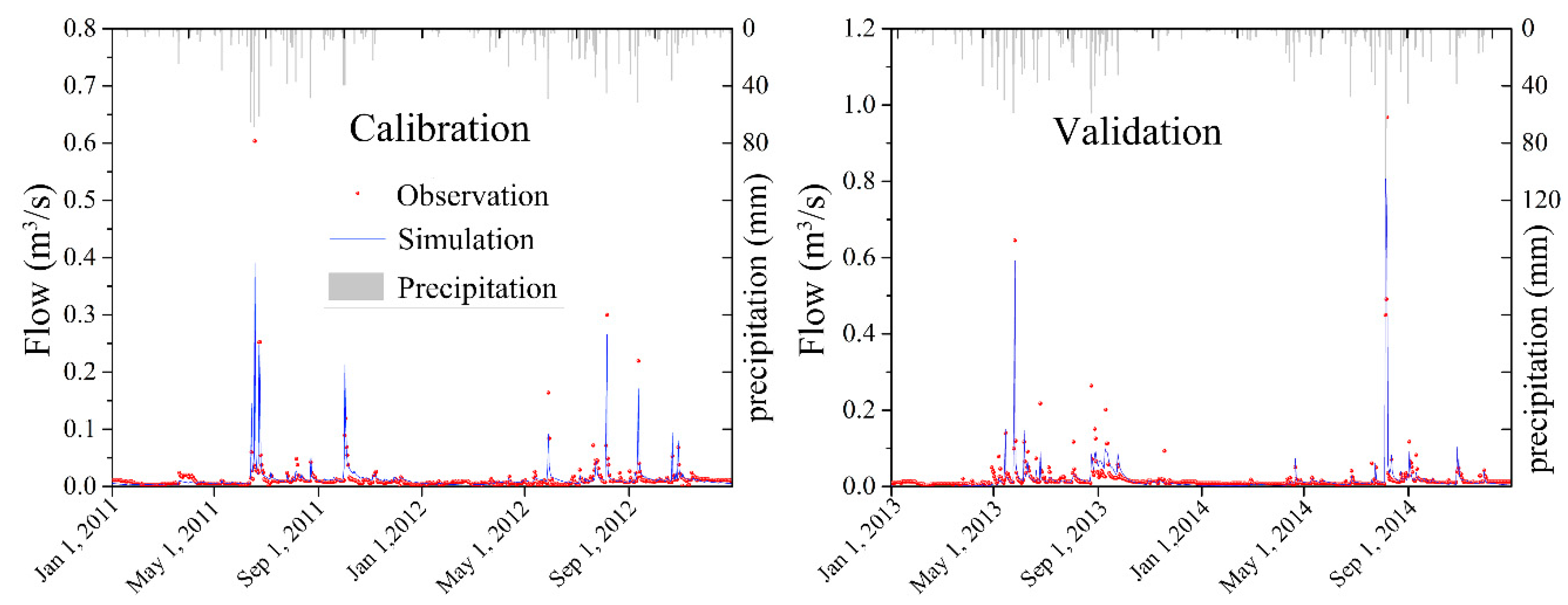
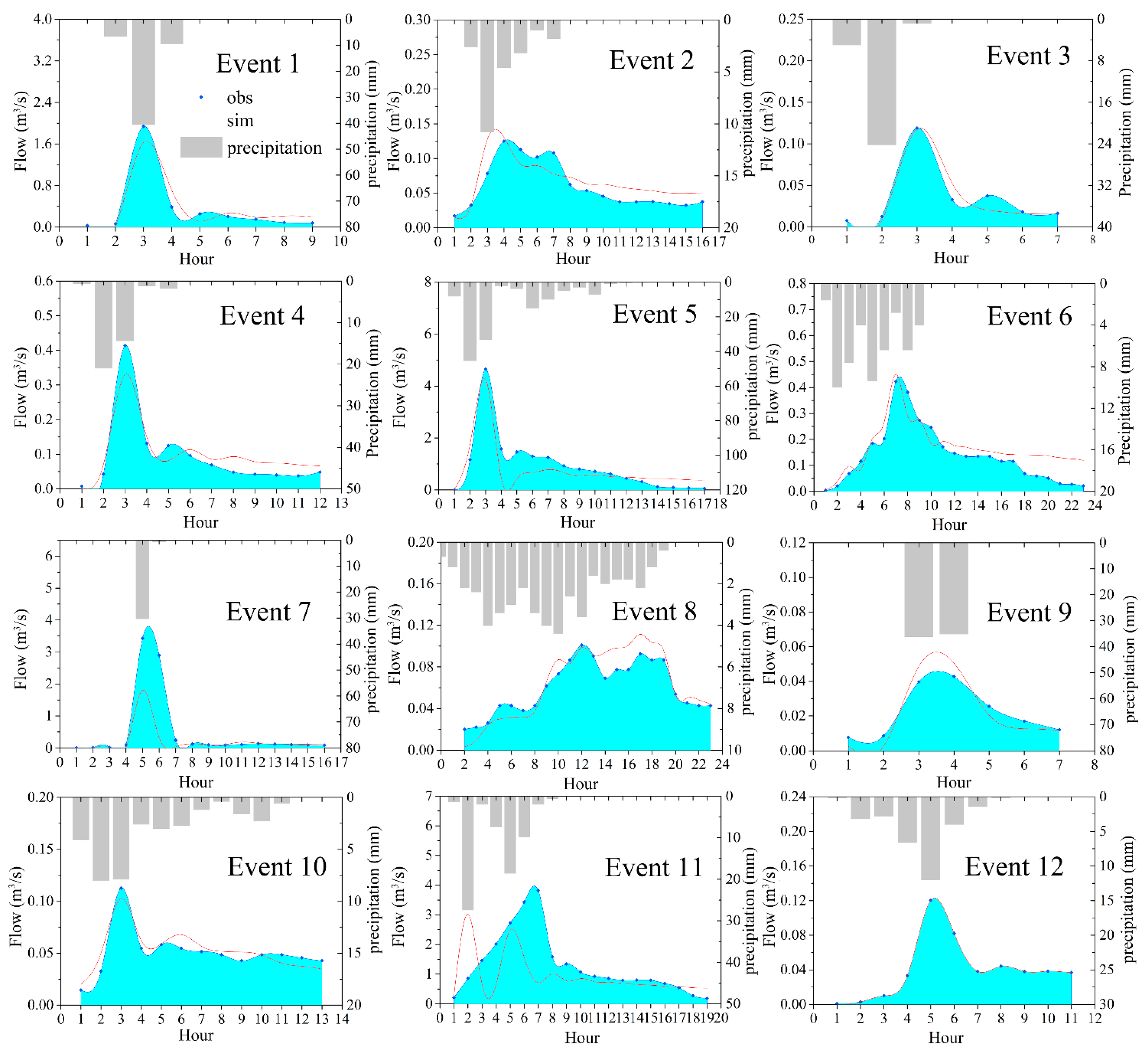
3.1. Comparison of Parameter Calibration

Generally, both the continuous and event-based models performed well in calibration and validation in terms of goodness-of-fit metrics and the hydrographs comparison. Figure 5 shows the 600 parameter sets in the multi-objective Pareto front for the continuous modeling and event modeling. Events 1 to 6 were concurrently calibrated to search for the optimized solutions that minimize the three objectives for all types of rainfall–runoff events. Simulated daily flows with the BOP parameters in the Pareto sets are plotted against the observations in Figure 6. Generally, the simulated daily flows agreed very well with the observed flows over the whole time period. Simulated hourly flows calculated using the BOP parameter values in the Pareto sets are plotted against the observations in Figure 7 for the 12 rainfall–runoff events. The calibration results of the continuous and event-based modeling were further compared using the HSPEXP method and the three commonly-used goodness-of-fit statistics (R², NSE, and RMSE) in

Table 4. Summary of calibration statistics for the continuous modeling.

Measures	Observed	Simulated	Percent Error %	HSPEXP Performance Criteria
Total runoff (mm)	543.34	534.08	−1.70	√
Mean of highest 10% flows (m3)	0.05692	0.0535	−5.97	√
Mean of lowest 50% flows (m3)	0.0062	0.0059	−4.54	√
Seasonal volume error (mm)	297.25	268.43	−9.70	√
Mean of storm peaks (m3)	0.0960	0.0940	−2.06	√
Summer storm volume (mm)	50.13	46.24	−7.76	√
Coefficient of determination	0.83
Nash–Sutcliffe efficiency	0.82
Root mean square error	0.76

and

Table 5. Summary of calibration and validation statistics for the event condition.

Event	Start date	NSE	RMSE	R2	PFE a	SVE b	PTO c
1	28 August 2013	0.91	9.72	0.92	0.16	0.05	0
2	21 April 2014	0.65	1.13	0.71	0.04	0.13	0
3	20 July 2014	0.93	0.60	0.93	0.01	0.05	0
4	24 July 2014	0.90	2.11	0.93	0.20	0.10	0
5	5 August 2014	0.79	27.91	0.81	0.08	0.34	0
6	2 September 2014	0.73	3.22	0.82	0.07	0.22	0
7	25 June 2013	0.83	16.17	0.98	0.38	0.29	0
8	24 September 2013	0.74	0.71	0.92	0.10	0.05	5
9	15 April 2014	0.49	0.57	0.77	0.18	0.15	0
10	25 June 2014	0.83	0.48	0.84	0.07	0.04	0
11	7 August 2014	−0.1172	60.81	0.12	0.21	0.28	5
12	23 August 2014	0.82	0.60	0.95	0.25	0.02	0

^a PFE stands for peak flow error; ^b SVE stands for storm volume error; ^c PTO stands for peak time offset.

. The HSPF model showed good performances compared to literature regarding hydrological modelling using the HSPF model [57,58,59].

The comparison of parameter estimation in the different scenarios is an important way to build reliable models. The optimized ranges for each parameter were normalized for comparison and are plotted in Figure 8. The BOP values of the two conditions are also listed in Table 3. The water balance for each component in the two scenarios are presented in

Table 6. Water balance comparison between the continuous and event scenarios in pervious lands.

Water Balance	Forest		Tea		Agriculture		Urban
Surface flow	9.23%	20.9%	5.76%	30.13%	3.44%	27.53%	6.34%	8.44%
Interflow	2.69%	63.03%	4.34%	54.92%	6.11%	65.61%	2.75%	64.33%
Base flow	8.45%	1.31%	37.6%	1.95%	28.46%	0.03%	27.44%	6.06%
Deep aquifer	0.52%	2.65%	2.26%	2.92%	1.72%	0.08%	1.65%	5.72%
Total ET	79.1%	12.11%	50.04%	10.08%	60.26%	6.74%	61.82%	15.45%

For each type of land use, the left and right column list the percentage of each component in the continuous and the event-based conditions, respectively.

to support the data analysis. The similarity between the two scenarios in terms of optimized ranges and BOP values was high for DEEPFR and IRC. DEEPFR is highly dependent on the watershed topography, thus its value may be constant during changes in the two scenarios. The BOP values of DEEPFR (0.056 and 0.057) were both very small, which can be corroborated by the percentage of deep aquifer in the water balance. The BOP values of IRC in the two scenarios were both calibrated to the pre-defined minimum bound, indicating very steep slopes of recession limbs of hydrographs. The precipitation in the Zhangjiachong catchment is characterized by large peaks and sudden decreases. Thus, the low value of IRC was possibly due to the sensitive and fast response to rainfall in this small catchment. The BOP values of LZSN, UZSN, and INFILT in the continuous modeling were higher than those in the event-based modeling. The continuous scenario consisted primarily of dry seasons when the base flow represented a large portion of the streamflow. Rainfall–runoff events were much more likely to result in overland flow and interflow, which can be seen in Table 6. Thus, higher values of LZSN and UZSN in the continuous modeling led to more water being retained in the soil zones and being available for base flow. Lower values of INFILT in the event-based modeling led to more moistures in the upper zone and in interflow storage, therefore resulting in more overland flow and interflow.

The INTFW value under the continuous scenario was calibrated to the lower boundary, which shared the same or similar value as in previous studies [10,60,61,62]. However, in the event-based scenario, the BOP value of INTFW approached the upper boundary and the optimized ranges were beyond 40% of the normalized range. This was because even during the largest rainfall–runoff events, overland flow was small compared to interflow [63]. As an example, Table 6 shows that the interflow was more than twice the surface flow in forest lands during rainfall–runoff events, increasing INTFW results in the increase of interflow and decreasing direct overland flow. Two primary base flow-related parameters, AGWRC and KVARY, also showed obvious differences in the comparison. The calibrated values (either the BOP values or values in optimized ranges) of AGWRC and KVARY were both higher in the continuous scenario than in the event-based modeling. Importantly, base flow feeds streamflow during low-rainfall seasons, thus representing a major part in the continuous scenario [64,65]. On the basis of the water balance calculation, base flow was much higher than the combination of surface flow and interflow in tea, agriculture, and urban lands of the pervious areas. Therefore, the values of AGWRC and KVARY were increased to supply more base flow in the continuous scenario. The above results of the parameter estimation show that calibrated parameter values apparently vary among the two scenarios. The study by Chu et al. [11] directly used the calibrated values of the event-based model for the continuous model, which caused the loss of simulation accuracy. In contrast, this study considered the parameter variation, which improved the model performances in the both scenarios.

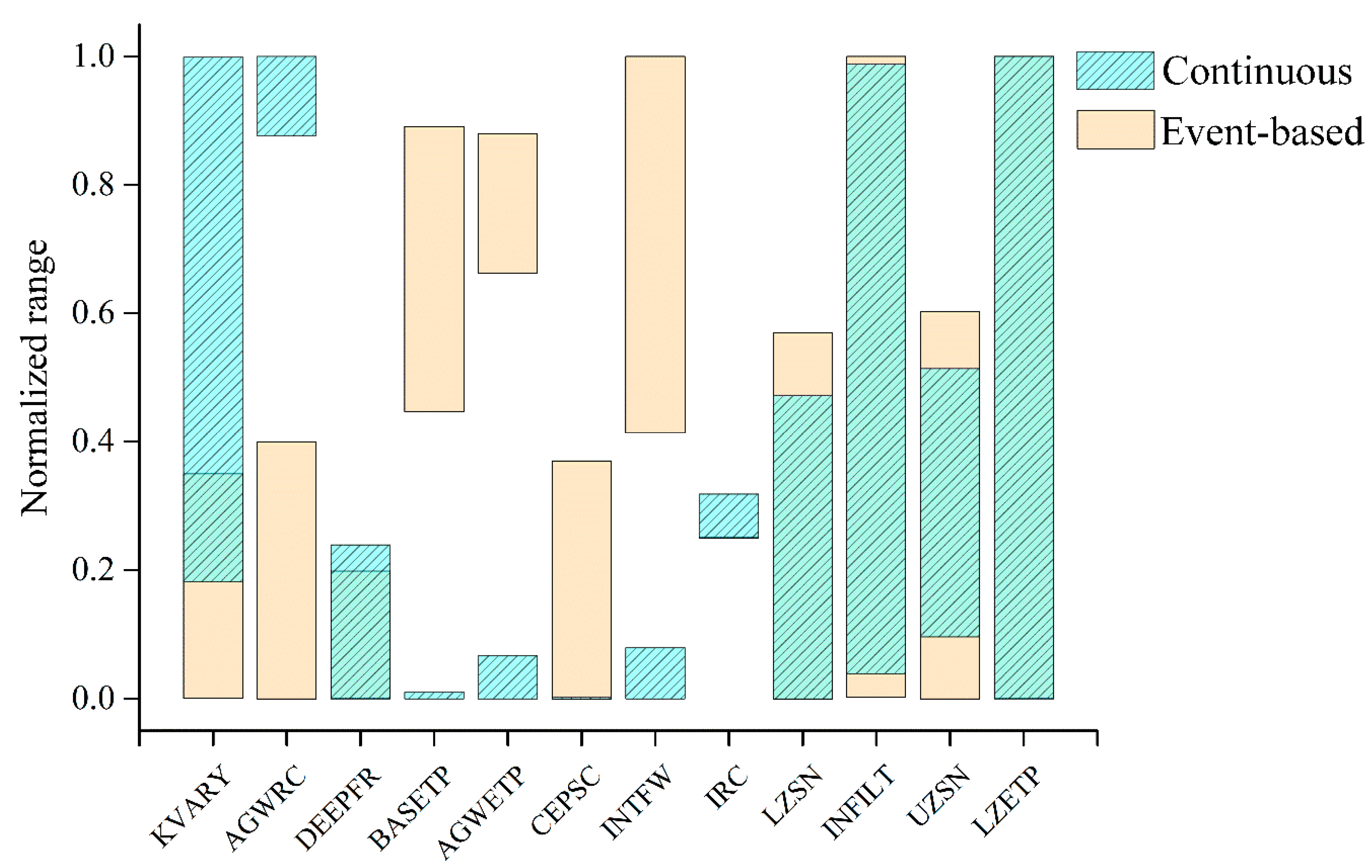
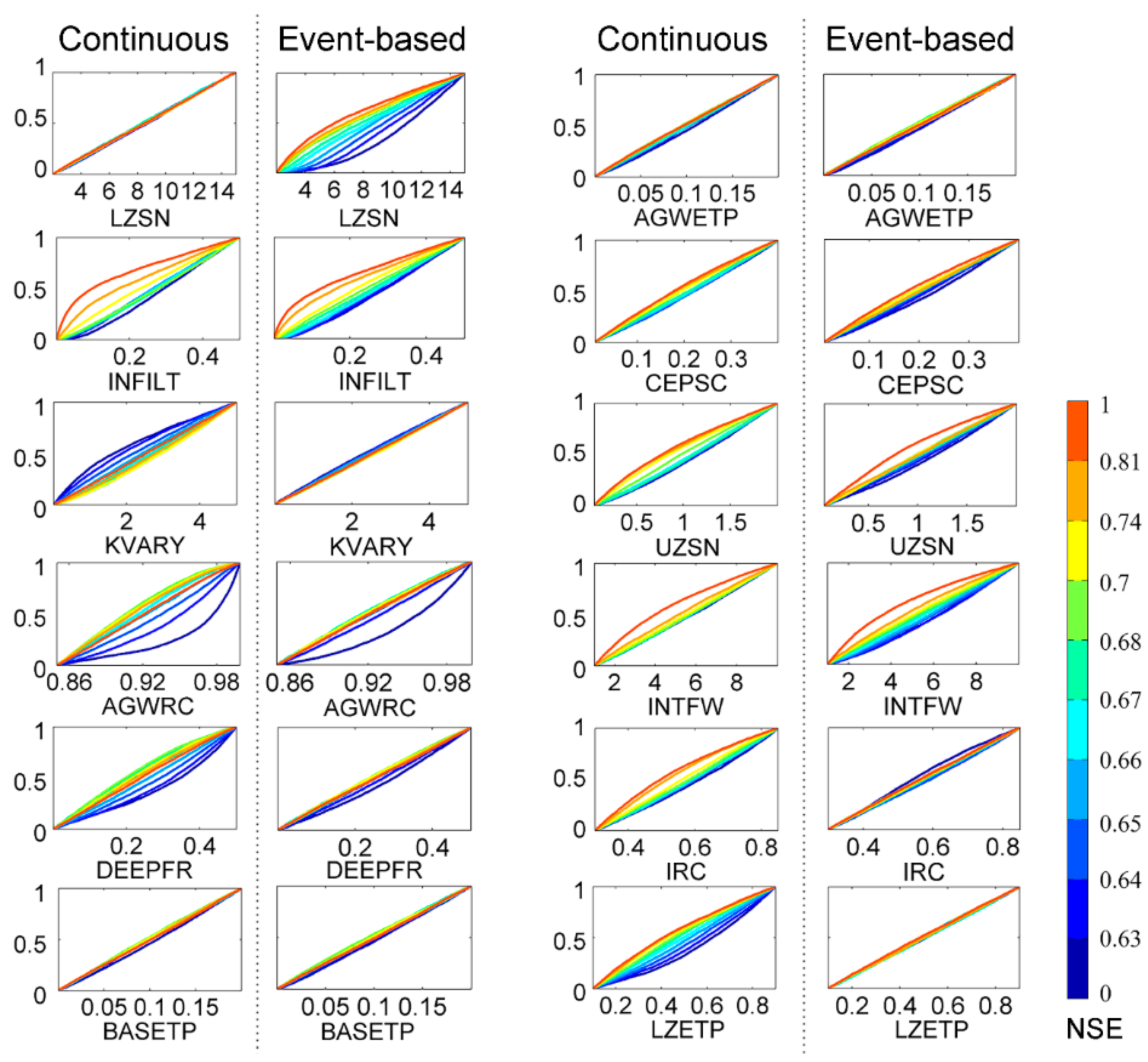
3.2. Comparison of Parameter Sensitivity

Figure 9 for the continuous modeling clearly indicates high sensitivity in eight parameters (i.e., INFILT, KVARY, AGWRC, DEEPFR, UZSN, INTFW, IRC, and LZETP) because the cumulative NSE values were apparently set apart from each other.

The high sensitivity of INFILT, INTFW, and UZSN is in accordance with reported literature on the use of HSPF in continuous modeling [58,66,67]. Each of the three parameters had a critical influence on the gravity drainage in the upper zone areas, and therefore indirectly affects overland flow, interflow, and base flow. During dry periods, the dominant mechanism of runoff generation is outflow from storage zones, which is influenced by the discharge rate constants, i.e., IRC, KVARY, and AGWRC. IRC is a critical outflow coefficient that controls interflow, while KVARY and AGWRC are parameter indexes that are directly related to the outflow amount of base flow. Therefore, these factors largely control the response of the hydrological modeling in the continuous scenario. The water balance calculation results indicated that water losses should be kept as much as possible to sustain enough streamflow for the continuous scenario. ET from low zone storages (controlled by LZETP) and infiltration to deep aquifers (controlled by DEEPFR) are sensitive processes.

For the event-based modeling, Figure 9 shows that five specific parameters (i.e., LZSN, INFILT, AGWRC, UZSN, and INTFW) were more sensitive than the other parameters. Parameters associated with quick hydrologic responses include INFILT, UZSN, and INTFW, which influenced direct runoff via surface runoff and interflow. The three parameters controlled the water amount in the upper zone and interflow zone. LZSN was very sensitive during event periods because gravity drainage became active for moisture re-distribution, which depended on LZS/LZSN in every vertical process. The sensitivity of the two outflow index parameters (i.e., IRC and AGWRC) was lower than that in the continuous modeling. Since the influence of outflow exceeding the storage maximum became weaker during rainfall–runoff events, they both showed a medium level of sensitivity.

The comparison of parameter sensitivity demonstrated that gravity drainage and overflow from soil storage were two of the main runoff generation processes in the HSPF model. The most notable difference between the two scenarios was the sensitivity of LZSN. The lower zone inflow is the sum of infiltration, percolation, lower zone lateral inflow, and irrigation application. It flows into the lower zone storage (LZS) that is based on the lower zone storage ratio of LZS/LZSN. It is likely that the LZS was primarily affected by current storage alone rather than by the inflow in the continuous modeling. However, during rainfall–runoff events, LZSN became sensitive since the LZS was influenced by both the current storage amount and gravity drainage. Based on the comparison results, the lower zone parameters (LZSN) were unlikely to be highly sensitive at any time. The other obvious difference was the sensitivity of LZETP. The lower zone was the most important storage where ET was very likely to occur. ET from the lower zone was higher than that from the other storages, but its influence was represented by the LZETP parameter. In the continuous scenario, water was possibly kept in the lower zone. The variation of LZETP values will lead to obvious variation in the lower zone storage, and then remarkably affect streamflow. However, during rainfall–runoff events, the available moisture from precipitation becomes sufficient to match the observed streamflow. The amount of water loss via ET becomes trivial compared to gravity drainage and overflow exceeding the storage maximum. Thus, LZETP is inactive in the event-based modeling. This comparison results of parameter sensitivity indicated that the parameters LZSN and LZETP were identified as event-dependent parameters, which is a significant consequence of interest to hydrologists using the HSPF model. It must be kept in mind that parameters that are inherently event-dependent should be updated in model applications between the two scenarios.

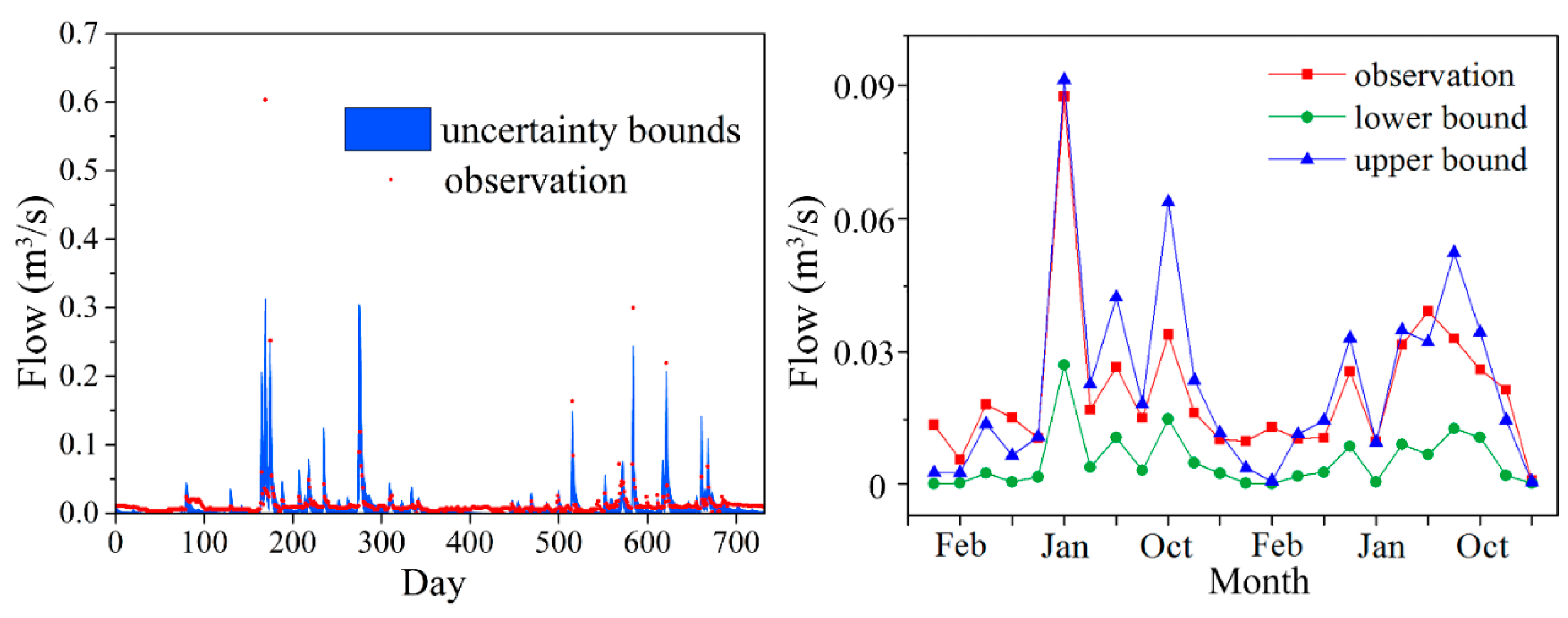
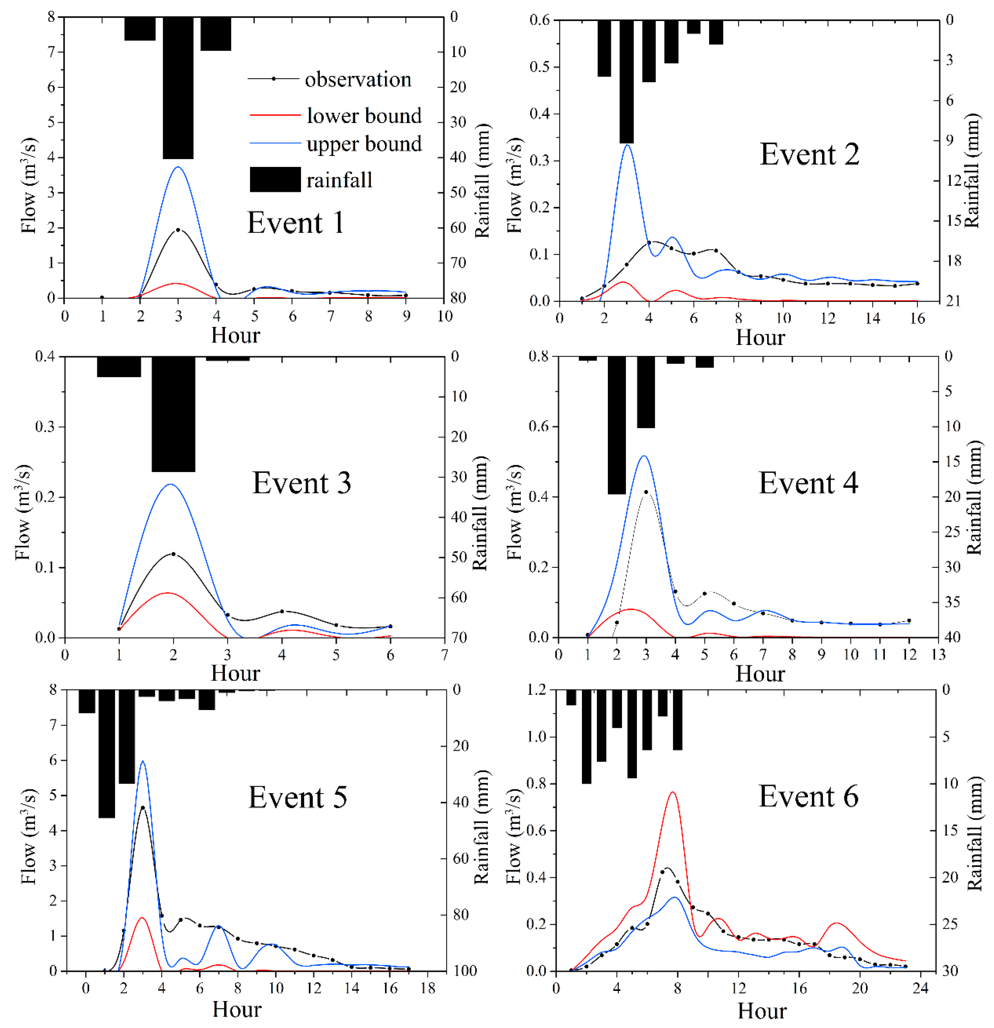
3.3. Comparison of Uncertainty Quantification

This section highlights the comparison of predictive uncertainty stemming from parameters in the two scenarios. The 95 PPU bounds were calculated using the 2.5% and 97.5% quantiles of the cumulative density distribution of acceptable results. The 95 PPU bounds (seen in Figure 10 and Figure 11) were used to determine the extent to which parameter uncertainty affects the model performance. The calculated p-factors and r-factors are presented in

Table 7. Measures for uncertainty analysis in the continuous and event-based modeling.

Scenario	Period	p-Factor (%)	r-Factor
Continuous	2011–2012 (daily)	40.25	2.58
	2011–2012 (monthly)	70.83	0.85
Event-based	Event 1 (Very heavy)	44.44	1.20
	Event 2 (Medium)	68.75	0.52
	Event 3 (Heavy)	33.3	1.13
	Event 4 (Heavy)	41.67	1.21
	Event 5 (Extremely heavy)	41.17	1.79
	Event 6 (Heavy)	65	1.17

. More observed data falling inside the 95 PPU bounds indicates higher p-factor values and better performances of the GLUE method. In the continuous modeling of daily flows, more than half of the observations fell outside the corresponding 95 PPU bounds. A similar result was obtained for the events characterized by heavy, very heavy, and extremely heavy conditions. The relatively low p-factors imply that the input or structure uncertainties may have dominated. Simulated data that falls outside bounds is a reflection of model structural error and possible inconsistencies in the data that is not being properly reflected in parameter sampling. However, the 95 PPU bounds of the monthly flow bracketed 70.83% of the observations, indicating a relatively high p-factor and that the parameter uncertainty contributed the most. The r-factor also showed a better simulation performance for the monthly flow with the HSPF model, which is in accordance with other studies [47,48]. This difference between the daily and monthly simulation is attributed to the fact that the monthly flow is a lumped data series that is very likely to mask the unexpected daily results caused by the input and structural uncertainties.

In Figure 10 for the daily simulation, some extremely high flows corresponding to large precipitation inputs were significantly underestimated (i.e., the observed daily flows were much higher than the 97.5% upper bound). This temporal variation presented an evidently clear relationship between precipitation input and predictive uncertainty. This could be explained by the fact that uncertainty is inherent in the rainfall input due to its spatial and temporal variability [68]. The Zhangjiachong catchment had only one weather station, which may not be sufficient to represent the precipitation spatial variability. Thus, the input uncertainty may very likely be propagated to the prediction results. While considering the catchment area is rather small, the input uncertainty from precipitation would be minor. During low-flow periods, many observed data were also underestimated, which can be seen in the monthly trends of the uncertainty bounds, especially in January, February, and March. Low flows most likely come from soil, channel storage release, or groundwater contributions, which are influenced by the soil, topography, and land use characteristics [69]. The HSPF model uses the exponential decay function to calculate base flow discharge. The research by Schultz et al. [70] used a power law storage–discharge function to replace the original equation. Improvements of model performances were achieved, which reflect the structural uncertainty rooted in the HSPF model.

Figure 11 illustrates the simulated hourly flows at the 95% quantile against observations for each of the six calibrated events. The overall performance of the event-based simulation was better than that of the daily simulation according to p-factors and r-factors. The observed peak flows were all bracketed by the uncertainty bands, implying the robust ability of the HSPF model in simulating peak flows in rainfall–runoff events. The event-based model showed the best performance for the medium events (event 2) with p-factor and r-factor values of 68.75% and 0.52, respectively. Generally, the performance of GLUE estimation decreased as the precipitation became intense. It is worth noting that at the beginning of rainfall–runoff events, the uncertainty bounds were often too narrow to cover the observed values. Similar outcomes were found in Sun et al. [71] in a context of GLUE application on streamflow forecasting in an urbanized catchment. Vezzaro and Mikkelsen [72] conducted uncertainty assessment for simulating micropollutants in stormwater runoff. These deficiencies of the results revealed the structure error of the models on the event basis. In rising limbs of rainfall–runoff events, the precipitation amount is rather small. Parameters related to moisture distribution and runoff generation are supposed to be dominant but cannot be fully activated at the initial event stage. Besides that, the characteristics of the analyzed dataset may also contribute to the deficiencies. The initial flows are rather small in magnitude and proportion compared to the others, which may be treated as outliers in constraining uncertainty bounds by the GLUE method.

4. Conclusions

A comparison-based procedure highlights the importance of comparing event-based and continuous modeling of streamflow in terms of parameter estimation and uncertainty analysis. This was achieved by using the HSPF model on a small catchment to explore the changes of parameter values, parameter sensitivity, and predictive uncertainty across different hydrologic scenarios. In the continuous and event-based modeling, the complexity of the climatic forcing caused differences in the parameter estimation and predictive uncertainty. Calibrated parameters related to base flow (i.e., AGWRC and KVARY) and moisture distribution (e.g., INTFW) showed marked differences between the continuous and event-based scenarios. Gravity drainage and storage outflow were the primary runoff generation mechanisms for both scenarios. LZSN and LZETP were identified as event-dependent parameters. The overall performance of the event-based simulation was better than that of the daily simulation for streamflow based on the generalized likelihood uncertainty estimation (GLUE). The GLUE analysis also indicated that the performance of the continuous model was limited by several extreme events and low flows. In the event-based scenario, HSPF model performances decreased as the precipitation became intense in the event-based modeling. The structure error of the HSFP model was recognized at the initial phrase of the rainfall-event period. These findings enable an improved understanding of parameter behavior in the HSPF model application and the identification of dominant processes under different hydrological scenarios.

References

1. Westerberg, I.K.; Guerrero, J.-L.; Younger, P.M.; Beven, K.J.; Seibert, J.; Halldin, S.; Freer, J.E.; Xu, C.-Y. Calibration of hydrological models using flow-duration curves. Hydrol. Earth Syst. Sci. 2011, 15, 2205–2227. [Google Scholar] [CrossRef] [Green Version]
2. Amaguchi, H.; Kawamura, A.; Olsson, J.; Takasaki, T. Development and testing of a distributed urban storm runoff event model with a vector-based catchment delineation. J. Hydrol. 2012, 420–421, 205–215. [Google Scholar] [CrossRef]
3. Wellen, C.; Arhonditsis, G.B.; Long, T.; Boyd, D. Accommodating environmental thresholds and extreme events in hydrological models: A Bayesian approach. J. Great Lakes Res. 2014, 40, 102–116. [Google Scholar] [CrossRef]
4. Wang, L.; van Meerveld, H.J.; Seibert, J. When should stream water be sampled to be most informative for event-based, multi-criteria model calibration? Hydrol. Res. 2017, 48, 1566–1584. [Google Scholar] [CrossRef] [Green Version]
5. Stephens, C.M.; Johnson, F.M.; Marshall, L.A. Implications of future climate change for event-based hydrologic models. Adv. Water Resour. 2018, 119, 95–110. [Google Scholar] [CrossRef]
6. Yu, D.; Xie, P.; Dong, X.; Hu, X.; Liu, J.; Li, Y.; Peng, T.; Ma, H.; Wang, K.; Xu, S. Improvement of the SWAT model for event-based flood simulation on a sub-daily timescale. Hydrol. Earth Syst. Sci. 2018, 22, 5001–5019. [Google Scholar] [CrossRef]
7. Qiu, J.; Shen, Z.; Wei, G.; Wang, G.; Xie, H.; Lv, G. A systematic assessment of watershed-scale nonpoint source pollution during rainfall-runoff events in the Miyun Reservoir watershed. Environ. Sci. Pollut. Res. 2018, 25, 6514–6531. [Google Scholar] [CrossRef]
8. Yao, C.; Zhang, K.; Yu, Z.; Li, Z.; Li, Q. Improving the flood prediction capability of the Xinanjiang model in ungauged nested catchments by coupling it with the geomorphologic instantaneous unit hydrograph. J. Hydrol. 2014, 517, 1035–1048. [Google Scholar] [CrossRef]
9. Borah, D.K.; Arnold, J.G.; Bera, M.; Krug, E.C.; Liang, X.-Z. Storm Event and Continuous Hydrologic Modeling for Comprehensive and Efficient Watershed Simulations. J. Hydrol. Eng. 2007, 12, 605–616. [Google Scholar] [CrossRef] [Green Version]
10. Ribarova, I.; Ninov, P.; Cooper, D. Modeling nutrient pollution during a first flood event using HSPF software: Iskar River case study, Bulgaria. Ecol. Model. 2008, 211, 241–246. [Google Scholar] [CrossRef]
11. Chu, X.; Steinman, A. Event and Continuous Hydrologic Modeling with HEC-HMS. J. Irrig. Drain. Eng. 2009, 135, 119–124. [Google Scholar] [CrossRef]
12. De Silva, M.M.G.T.; Weerakoon, S.B.; Herath, S. Modeling of Event and Continuous Flow Hydrographs with HEC–HMS: Case Study in the Kelani River Basin, Sri Lanka. J. Hydrol. Eng. 2014, 19, 800–806. [Google Scholar] [CrossRef]
13. Huang, P.; Li, Z.; Yao, C.; Li, Q.; Yan, M. Spatial combination modeling framework of saturation-excess and infiltration-excess runoff for semihumid watersheds. Adv. Meteorol. 2016, 2016. [Google Scholar] [CrossRef]
14. Pfannerstill, M.; Guse, B.; Reusser, D.; Fohrer, N. Process verification of a hydrological model using a temporal parameter sensitivity analysis. Hydrol. Earth Syst. Sci. 2015, 19, 4365–4376. [Google Scholar] [CrossRef] [Green Version]
15. Kirchner, J.W. Getting the right answers for the right reasons: Linking measurements, analyses, and models to advance the science of hydrology. Water Resour. Res. 2006, 42. [Google Scholar] [CrossRef] [Green Version]
16. Herman, J.D.; Reed, P.M.; Wagener, T. Time-varying sensitivity analysis clarifies the effects of watershed model formulation on model behavior. Water Resour. Res. 2013, 49, 1400–1414. [Google Scholar] [CrossRef] [Green Version]
17. Guse, B.; Reusser, D.E.; Fohrer, N. How to improve the representation of hydrological processes in SWAT for a lowland catchment–temporal analysis of parameter sensitivity and model performance. Hydrol. Process. 2014, 28, 2651–2670. [Google Scholar] [CrossRef]
18. Xie, H.; Shen, Z.; Chen, L.; Qiu, J.; Dong, J. Time-varying sensitivity analysis of hydrologic and sediment parameters at multiple timescales: Implications for conservation practices. Sci. Total Environ. 2017, 598, 353–364. [Google Scholar] [CrossRef]
19. Garambois, P.A.; Roux, H.; Larnier, K.; Castaings, W.; Dartus, D. Characterization of process-oriented hydrologic model behavior with temporal sensitivity analysis for flash floods in Mediterranean catchments. Hydrol. Earth Syst. Sci. 2013, 17, 2305–2322. [Google Scholar] [CrossRef] [Green Version]
20. Srivastava, V.; Graham, W.; Muñoz-Carpena, R.; Maxwell, R.M. Insights on geologic and vegetative controls over hydrologic behavior of a large complex basin—Global Sensitivity Analysis of an integrated parallel hydrologic model. J. Hydrol. 2014, 519, 2238–2257. [Google Scholar] [CrossRef]
21. Herman, J.D.; Kollat, J.B.; Reed, P.M.; Wagener, T. From maps to movies: High-resolution time-varying sensitivity analysis for spatially distributed watershed models. Hydrol. Earth Syst. Sci. 2013, 17, 5109–5125. [Google Scholar] [CrossRef]
22. Jiang, S.Y.; Zhang, Q.; Werner, A.D.; Wellen, C.; Jomaa, S.; Zhu, Q.D.; Büttner, O.; Meon, G.; Rode, M. Effects of stream nitrate data frequency on watershed model performance and prediction uncertainty. J. Hydrol. 2019, 569, 22–36. [Google Scholar] [CrossRef]
23. Wellen, C.; Kamran-Disfani, A.-R.; Arhonditsis, G.B. Evaluation of the Current State of Distributed Watershed Nutrient Water Quality Modeling. Environ. Sci. Technol. 2015, 49, 3278–3290. [Google Scholar] [CrossRef] [PubMed]
24. Bicknell, B.R.; Imhoff, J.C.; Kittle, J.L., Jr.; Donigian, A.S., Jr.; Johanson, R.C. Hydrological Simulation Program-FORTRAN. User’s Manual for Release 11; USEPA: Athens, GA, USA, 1997.
25. Arnold, J.G.; Srinivasan, R.; Muttiah, R.S.; Williams, J.R. Large area hydrologic modeling and assessment part I: Model development 1. JAWRA J. Am. Water Resour. Assoc. 1998, 34, 73–89. [Google Scholar] [CrossRef]
26. Hydrologic Engieering Center (US). The Hydrologic Modeling System (HEC-HMS); US Army Corps of Engineers, Hydrologic Engineering Center: Davis, CA, USA, 2001. [Google Scholar]
27. Rossman, L.A. Storm Water Management Model User’s Manual, Version 5.0; National Risk Management Research Laboratory, Office of Research and Development: Cincinnati, OH, USA, 2009.
28. Lindström, G.; Pers, C.; Rosberg, J.; Strömqvist, J.; Arheimer, B. Development and testing of the HYPE (Hydrological Predictions for the Environment) water quality model for different spatial scales. Hydrol. Res. 2010, 41, 295–319. [Google Scholar] [CrossRef]
29. Refsgaard, J.C.; Storm, B. Computer Models of Watershed Hydrology; Water Resources Publications: Fort Collins, CO, USA, 1995; pp. 809–846. [Google Scholar]
30. Berndt, M.E.; Rutelonis, W.; Regan, C.P. A comparison of results from a hydrologic transport model (HSPF) with distributions of sulfate and mercury in a mine-impacted watershed in northeastern Minnesota. J. Environ. Manag. 2016, 181, 74–79. [Google Scholar] [CrossRef] [PubMed] [Green Version]
31. Li, Z.; Luo, C.; Jiang, K.; Wan, R.; Li, H. Comprehensive Performance Evaluation for Hydrological and Nutrients Simulation Using the Hydrological Simulation Program–Fortran in a Mesoscale Monsoon Watershed, China. Int. J. Environ. Res. Public. Health 2017, 14, 1599. [Google Scholar] [CrossRef]
32. Fonseca, A.; Boaventura, R.A.R.; Vilar, V.J.P. Integrating water quality responses to best management practices in Portugal. Environ. Sci. Pollut. Res. 2018, 25, 1587–1596. [Google Scholar] [CrossRef]
33. Ouyang, Y.; Parajuli, P.B.; Feng, G.; Leininger, T.D.; Wan, Y.; Dash, P. Application of Climate Assessment Tool (CAT) to estimate climate variability impacts on nutrient loading from local watersheds. J. Hydrol. 2018, 563, 363–371. [Google Scholar] [CrossRef]
34. Ahn, S.-R.; Kim, S.-J. The Effect of Rice Straw Mulching and No-Tillage Practice in Upland Crop Areas on Nonpoint-Source Pollution Loads Based on HSPF. Water 2016, 8, 106. [Google Scholar] [CrossRef]
35. Fonseca, A.R.; Santos, M.; Santos, J.A. Hydrological and flood hazard assessment using a coupled modelling approach for a mountainous catchment in Portugal. Stoch. Environ. Res. Risk Assess. 2018, 32, 2165–2177. [Google Scholar] [CrossRef]
36. Xie, H.; Wei, G.; Shen, Z.; Dong, J.; Peng, Y.; Chen, X. Event-based uncertainty assessment of sediment modeling in a data-scarce catchment. CATENA 2019, 173, 162–174. [Google Scholar] [CrossRef]
37. Lin, S.; Iqbal, J.; Hu, R.; Shaaban, M.; Cai, J.; Chen, X. Nitrous Oxide Emissions from Yellow Brown Soil as Affected by Incorporation of Crop Residues with Different Carbon-to-Nitrogen Ratios: A Case Study in Central China. Arch. Environ. Contam. Toxicol. 2013, 65, 183–192. [Google Scholar] [CrossRef] [PubMed]
38. VanWoert, N.D.; Rowe, D.B.; Andresen, J.A.; Rugh, C.L.; Fernandez, R.T.; Xiao, L. Green Roof Stormwater Retention. J. Environ. Qual. 2005, 34, 1036–1044. [Google Scholar] [CrossRef] [PubMed]
39. Voyde, E.; Fassman, E.; Simcock, R. Hydrology of an extensive living roof under sub-tropical climate conditions in Auckland, New Zealand. J. Hydrol. 2010, 394, 384–395. [Google Scholar] [CrossRef]
40. Stovin, V.; Vesuviano, G.; Kasmin, H. The hydrological performance of a green roof test bed under UK climatic conditions. J. Hydrol. 2012, 414–415, 148–161. [Google Scholar] [CrossRef]
41. Dunnett, N.; Nagase, A.; Booth, R.; Grime, P. Influence of vegetation composition on runoff in two simulated green roof experiments. Urban Ecosyst. 2008, 11, 385–398. [Google Scholar] [CrossRef]
42. Whittinghill, L.J.; Rowe, D.B.; Andresen, J.A.; Cregg, B.M. Comparison of stormwater runoff from sedum, native prairie, and vegetable producing green roofs. Urban Ecosyst. 2015, 18, 13–29. [Google Scholar] [CrossRef]
43. Chen, L.; Sun, C.; Wang, G.; Xie, H.; Shen, Z. Event-based nonpoint source pollution prediction in a scarce data catchment. J. Hydrol. 2017, 552, 13–27. [Google Scholar] [CrossRef]
44. Chen, L.; Sun, C.; Wang, G.; Xie, H.; Shen, Z. Modeling Multi-Event Non-Point Source Pollution in a Data-Scarce Catchment Using ANN and Entropy Analysis. Entropy 2017, 19, 265. [Google Scholar] [CrossRef]
45. Deb, K.; Agrawal, S.; Pratap, A.; Meyarivan, T. A Fast Elitist Non-dominated Sorting Genetic Algorithm for Multi-objective Optimization: NSGA-II. In Proceedings of the Parallel Problem Solving from Nature PPSN VI; Schoenauer, M., Deb, K., Rudolph, G., Yao, X., Lutton, E., Merelo, J.J., Schwefel, H.-P., Eds.; Springer: Berlin/Heidelberg, Germany, 2000; pp. 849–858. [Google Scholar]
46. Pfannerstill, M.; Guse, B.; Fohrer, N. Smart low flow signature metrics for an improved overall performance evaluation of hydrological models. J. Hydrol. 2014, 510, 447–458. [Google Scholar] [CrossRef]
47. Kim, S.M.; Benham, B.L.; Brannan, K.M.; Zeckoski, R.W.; Doherty, J. Comparison of hydrologic calibration of HSPF using automatic and manual methods. Water Resour. Res. 2007, 43. [Google Scholar] [CrossRef] [Green Version]
48. Lumb, A.M.; McCammon, R.B.; Kittle, J.L. Users Manual for an Expert System (HSPEXP) for Calibration of the Hydrological Simulation Program—Fortran; US Geological Survey Reston: Reston, Virginia, 1994.
49. Nash, J.E.; Sutcliffe, J.V. River flow forecasting through conceptual models part I—A discussion of principles. J. Hydrol. 1970, 10, 282–290. [Google Scholar] [CrossRef]
50. Hallema, D.W.; Moussa, R.; Andrieux, P.; Voltz, M. Parameterization and multi-criteria calibration of a distributed storm flow model applied to a Mediterranean agricultural catchment. Hydrol. Process. 2013, 27, 1379–1398. [Google Scholar] [CrossRef]
51. Song, X.; Zhang, J.; Zhan, C.; Xuan, Y.; Ye, M.; Xu, C. Global sensitivity analysis in hydrological modeling: Review of concepts, methods, theoretical framework, and applications. J. Hydrol. 2015, 523, 739–757. [Google Scholar] [CrossRef] [Green Version]
52. Spear, R.C.; Hornberger, G.M. Eutrophication in peel inlet—II. Identification of critical uncertainties via generalized sensitivity analysis. Water Res. 1980, 14, 43–49. [Google Scholar] [CrossRef]
53. Wagener, T.; Boyle, D.P.; Lees, M.J.; Wheater, H.S.; Gupta, H.V.; Sorooshian, S. A framework for development and application of hydrological models. Hydrol. Earth Syst. Sci. 2001, 5, 13–26. [Google Scholar] [CrossRef] [Green Version]
54. Pianosi, F.; Sarrazin, F.; Wagener, T. A Matlab toolbox for Global Sensitivity Analysis. Environ. Model. Softw. 2015, 70, 80–85. [Google Scholar] [CrossRef] [Green Version]
55. Beven, K.; Binley, A. The future of distributed models: Model calibration and uncertainty prediction. Hydrol. Process. 1992, 6, 279–298. [Google Scholar] [CrossRef]
56. Abbaspour, K.C. User Manual for SWAT-CUP: SWAT Calibration and Uncertainty Analysis Program; Swiss Federal Institute of Aquatic Science and Technology, Eawag: Duebendorf, Switzerland, 2007. [Google Scholar]
57. Fonseca, A.; Ames, D.P.; Yang, P.; Botelho, C.; Boaventura, R.; Vilar, V. Watershed model parameter estimation and uncertainty in data-limited environments. Environ. Model. Softw. 2014, 51, 84–93. [Google Scholar] [CrossRef]
58. Chung, E.-S.; Park, K.; Lee, K.S. The relative impacts of climate change and urbanization on the hydrological response of a Korean urban watershed. Hydrol. Process. 2011, 25, 544–560. [Google Scholar] [CrossRef]
59. Seong, C.; Her, Y.; Benham, B.L. Automatic calibration tool for Hydrologic Simulation Program-FORTRAN using a shuffled complex evolution algorithm. Water 2015, 7, 503–527. [Google Scholar] [CrossRef]
60. Hayashi, S.; Murakami, S.; Xu, K.-Q.; Watanabe, M. Simulation of the reduction of runoff and sediment load resulting from the Gain for Green Program in the Jialingjiang catchment, upper region of the Yangtze River, China. J. Environ. Manag. 2015, 149, 126–137. [Google Scholar] [CrossRef] [PubMed]
61. Baloch, M.A.; Ames, D.P.; Tanik, A. Hydrologic impacts of climate and land-use change on Namnam Stream in Koycegiz Watershed, Turkey. Int. J. Environ. Sci. Technol. 2015, 12, 1481–1494. [Google Scholar] [CrossRef]
62. Choi, W.; Deal, B.M. Assessing hydrological impact of potential land use change through hydrological and land use change modeling for the Kishwaukee River basin (USA). J. Environ. Manag. 2008, 88, 1119–1130. [Google Scholar] [CrossRef] [PubMed]
63. Verhagen, W. Wetland Restoration in an Agricultural Basin. Linking Hydrologic Response, Optimal Location, Ecosystem Services and Stakeholder Opinions. Master’s Thesis, Utrecht University Repository, Utrecht, The Netherlands, 2013. [Google Scholar]
64. Lott, D.A.; Stewart, M.T. Base flow separation: A comparison of analytical and mass balance methods. J. Hydrol. 2016, 535, 525–533. [Google Scholar] [CrossRef]
65. Risser, D.W.; Gburek, W.J.; Folmar, G.J. Comparison of Methods for Estimating Ground-Water Recharge and Base Flow at a Small Watershed Underlain by Fractured Bedrock in the Eastern United States; US Department of the Interior, US Geological Survey: Reston, VA, USA, 2005; Volume 5038.
66. Abdulla, F.; Eshtawi, T.; Assaf, H. Assessment of the Impact of Potential Climate Change on the Water Balance of a Semi-arid Watershed. Water Resour. Manag. 2009, 23, 2051–2068. [Google Scholar] [CrossRef]
67. Mishra, A.; Kar, S.; Singh, V.P. Determination of runoff and sediment yield from a small watershed in sub-humid subtropics using the HSPF model. Hydrol. Process. 2007, 21, 3035–3045. [Google Scholar] [CrossRef]
68. Shen, Z.; Chen, L.; Liao, Q.; Liu, R.; Hong, Q. Impact of spatial rainfall variability on hydrology and nonpoint source pollution modeling. J. Hydrol. 2012, 472–473, 205–215. [Google Scholar] [CrossRef]
69. Mohamoud, Y.M.; Parmar, R.; Wolfe, K.; Carleton, J. HSPF toolkit: A tool for stormwater management at the watershed scale. Proc. Water Environ. Fed. 2008, 2008, 421–431. [Google Scholar] [CrossRef]
70. Schultz, C.L.; Ahmed, S.N.; Mandel, R.; Moltz, H.L.N. Improvement in HSPF’s Low-Flow Predictions by Implementation of a Power Law Groundwater Storage-Discharge Relationship. JAWRA J. Am. Water Resour. Assoc. 2014, 50, 909–927. [Google Scholar] [CrossRef]
71. Sun, N.; Hong, B.; Hall, M. Assessment of the SWMM model uncertainties within the generalized likelihood uncertainty estimation (GLUE) framework for a high-resolution urban sewershed. Hydrol. Process. 2014, 28, 3018–3034. [Google Scholar] [CrossRef]
72. Vezzaro, L.; Mikkelsen, P.S. Application of global sensitivity analysis and uncertainty quantification in dynamic modelling of micropollutants in stormwater runoff. Environ. Model. Softw. 2012, 27–28, 40–51. [Google Scholar] [CrossRef]
Figure 1. Location, land use, and elevation of the Zhangjiachong catchment.
Water 11 00171 g001
Figure 2. Monthly distribution of event occurrence of different types.
Water 11 00171 g002
Figure 3. Water storages and movement represented in the PERLND module. ET: evapotranspiration, AGWS: active ground water storage, LZS: lower zone storage, UPS: upper zone storage, IFWS: interflow storage, SURS: surface detention storage, CEPS: Interception storage.
Water 11 00171 g003
Figure 4. Flowchart of the HSPF/NSGA-II calibration framework.
Water 11 00171 g004
Figure 5. Pareto sets achieved by the multi-objective calibration. The left part is for the continuous modeling, where green, blue, and red dots represent solutions those that achieved four, five, and six criteria of the HSEXP statistics, respectively. The right part is for the event-based modeling, where green dots represent all the Pareto solutions. The original MATLAB figure files (Pareto front-continuous scenario.fig and Pareto front-event-based scenario.fig) are provided as Supplementary Materials.
Water 11 00171 g005
Figure 6. Hyetograph, simulated and observed hydrographs in the calibration and validation periods for the continuous modeling.
Water 11 00171 g006
Figure 7. Hyetograph, and simulated and observed hydrographs in the calibration and validation periods for the 12 rainfall–runoff events.
Water 11 00171 g007
Figure 8. Comparison of the optimized parameter ranges between the continuous and event-based modeling.
Water 11 00171 g008
Figure 9. Comparison of parameter sensitivity between the continuous and event-based modeling Cumulative normalized Nash–Sutcliffe efficiency were plotted against parameter values. Parameter populations from best to worst are ranked and divided into ten bins of equal size.
Water 11 00171 g009
Figure 10. Observations and 95 PPU bounds of streamflow in the continuous modeling. The left and right parts present results of daily and monthly simulation, respectively.
Water 11 00171 g010
Figure 11. Hyetograph, observations, and 95 PPU bounds of streamflow in the representative rainfall–runoff events.
Water 11 00171 g011