Development and Application of Advanced Muskingum Flood Routing Model Considering Continuous Flow


Abstract
1. Introduction
2. Materials and Methods
2.1. Overview
2.2. Advanced Nonlinear Muskingum Model Considering Continuous Flow
2.3. Numerical Method for Parameter Estimation
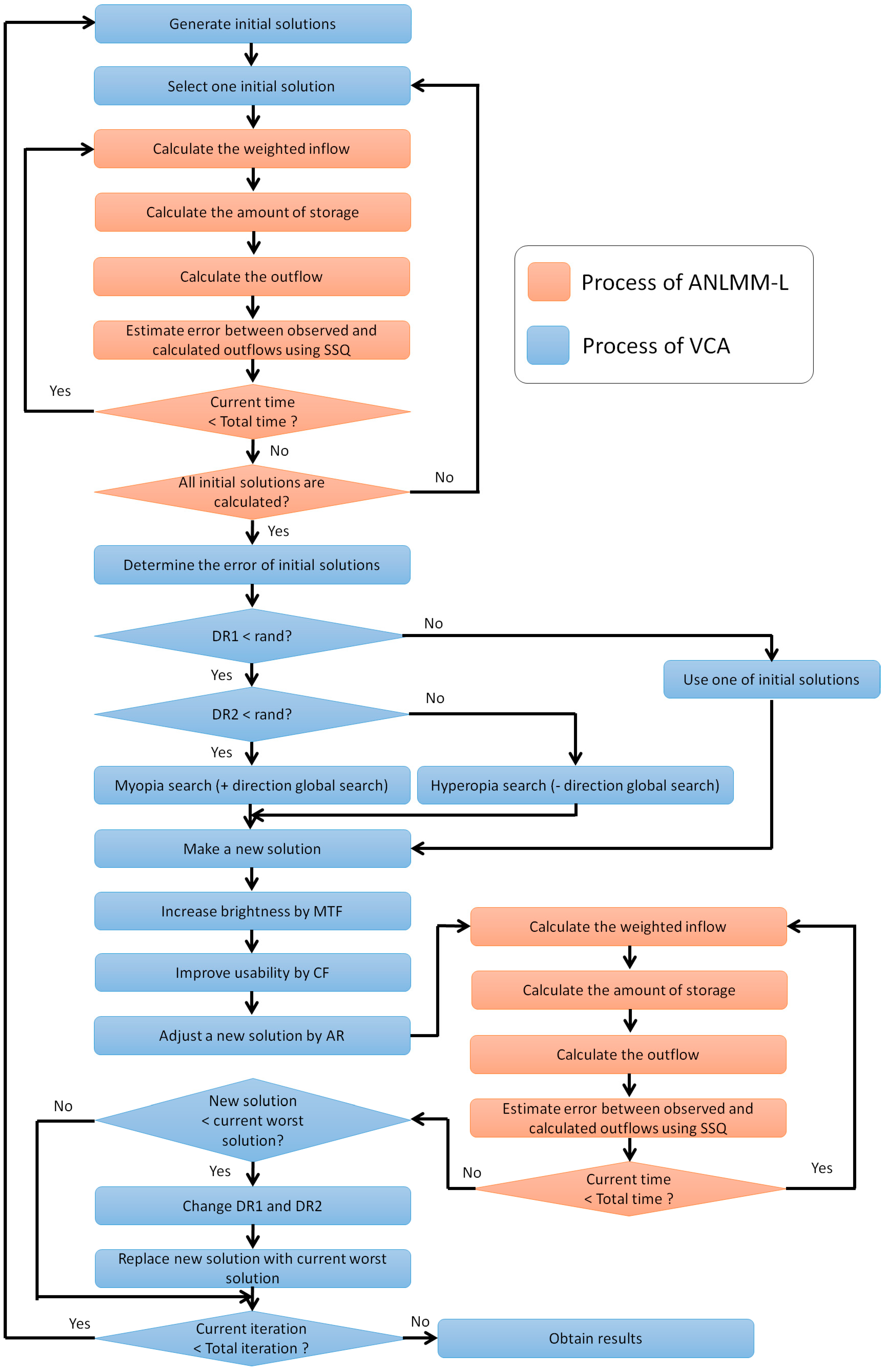
2.4. Vision Correction Algorithm
- Generate initial solutions
- Calculate the fitness of solutions using the objective function
- Generate new solution
- Compare new solution with current worst solution
- Determine the replacement between two solutions
- Repeat steps 2–5 if iteration process is not finished.
3. Results
3.1. Application of Wilson Flood Data
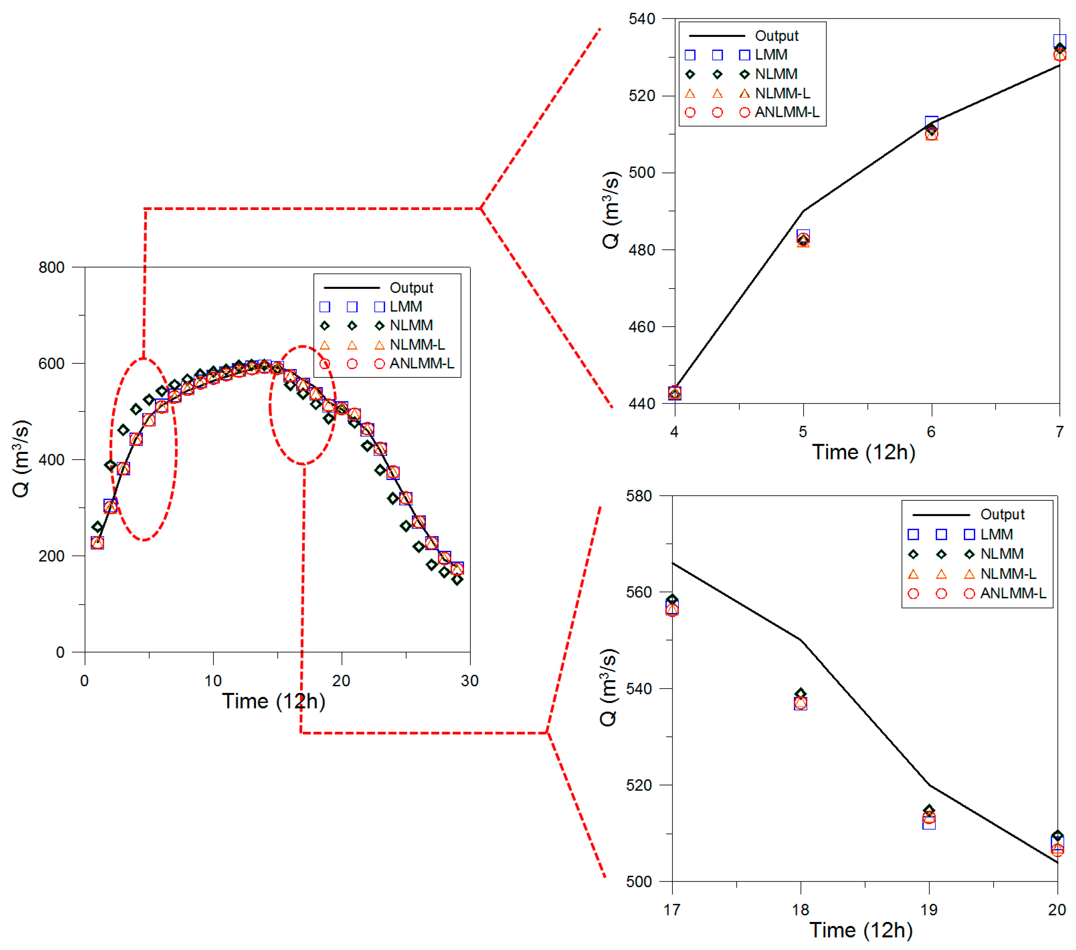
3.2. Application of Flood Data by Wang et al. (2009)
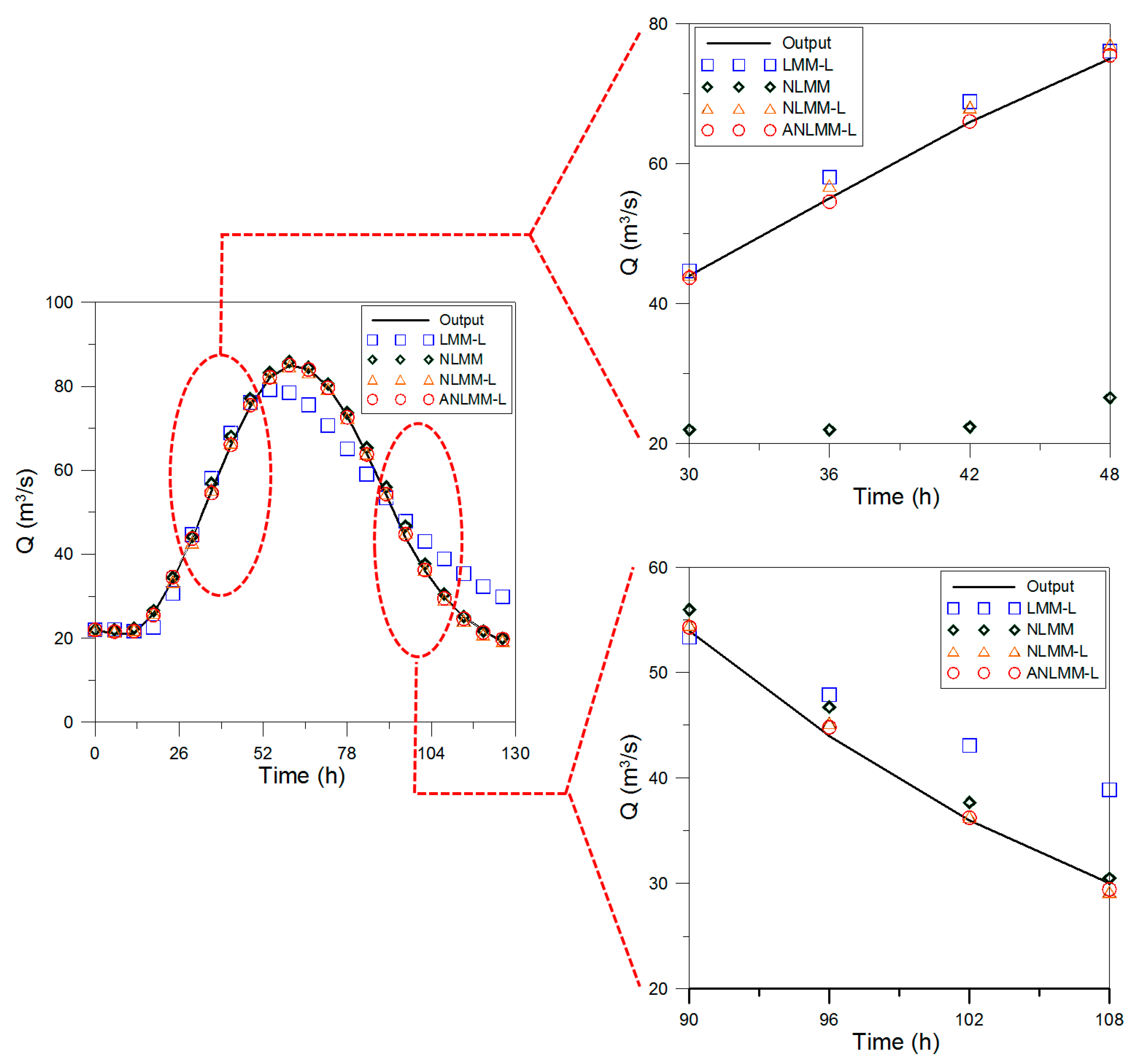
3.3. Application of Flood Data for River Wye December in 1960
3.4. Application of Sutculer Flood Data
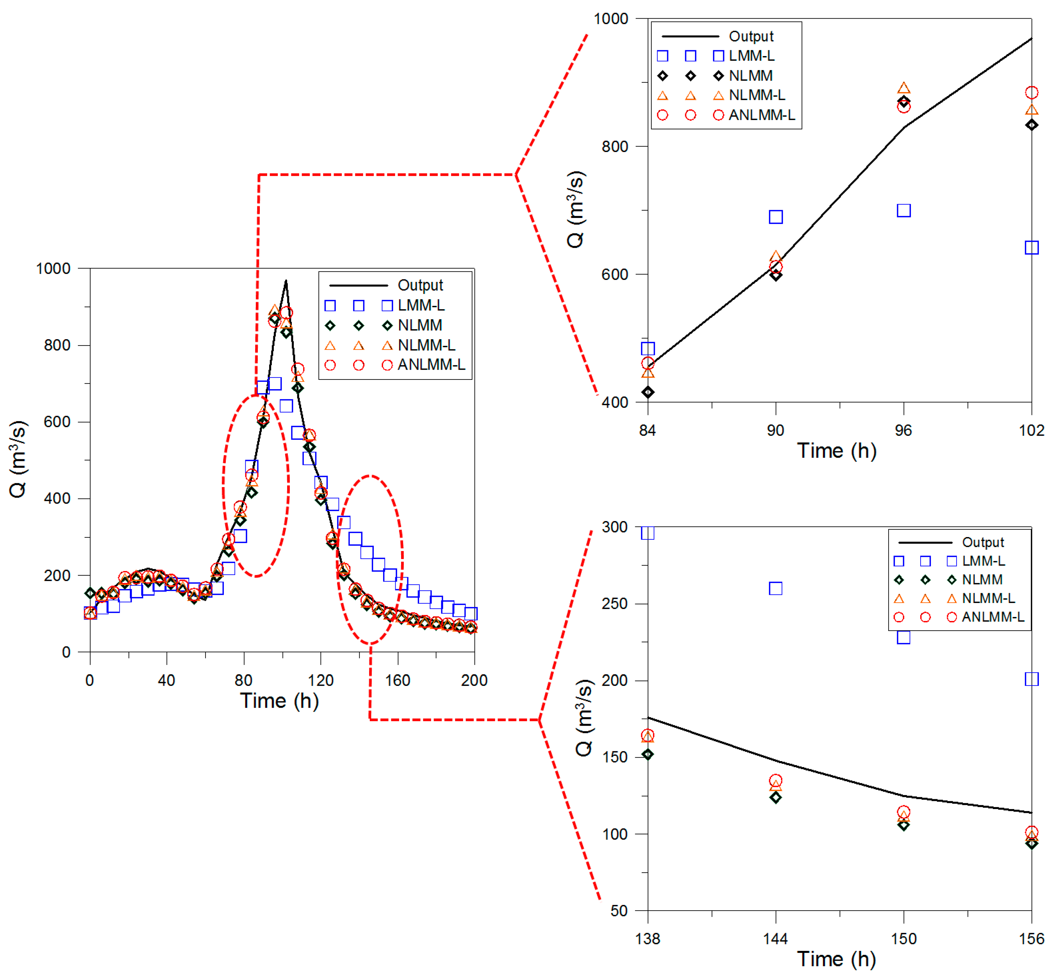
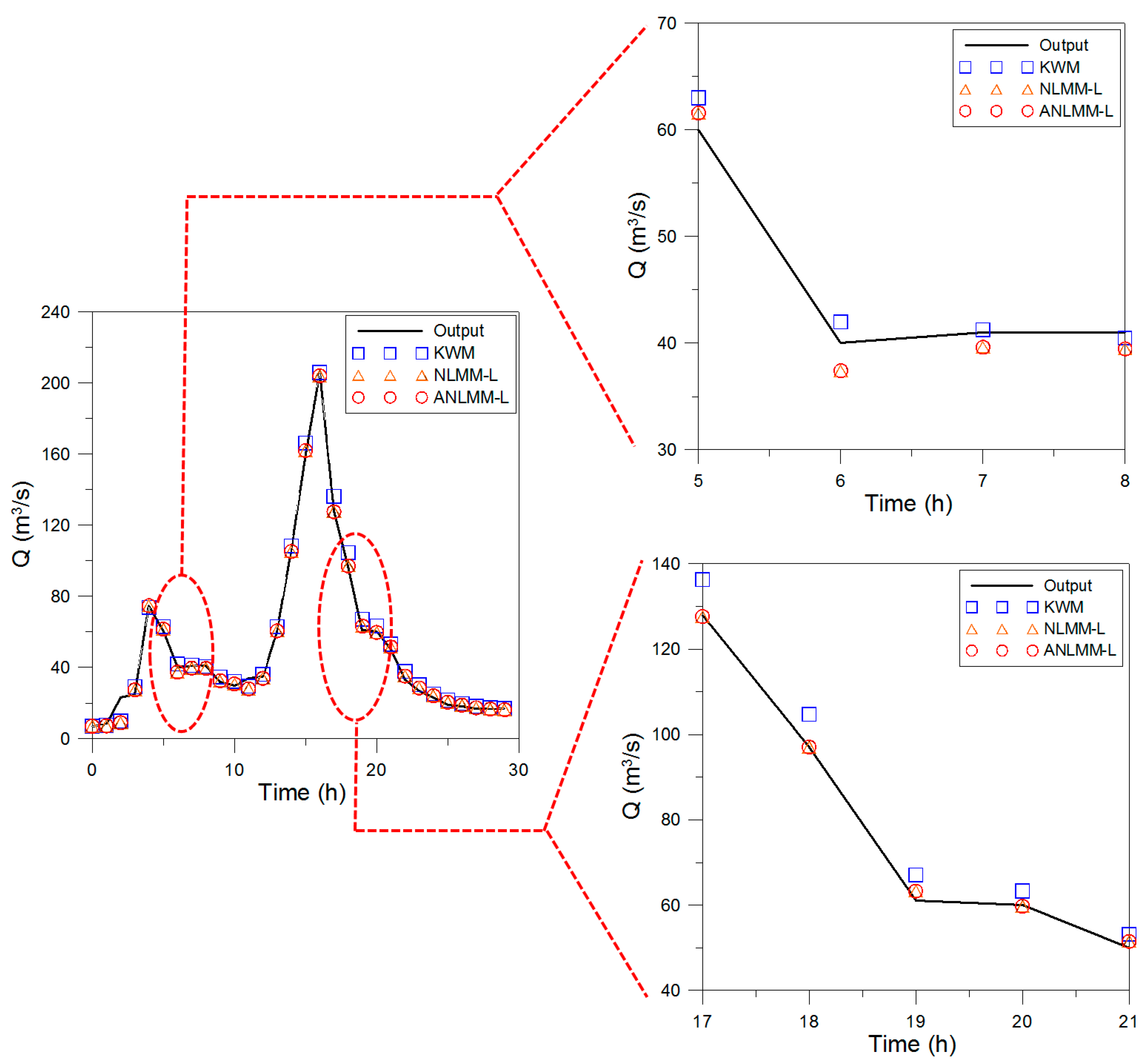
3.5. Application of the Flood Data for River Wyre October in 1982
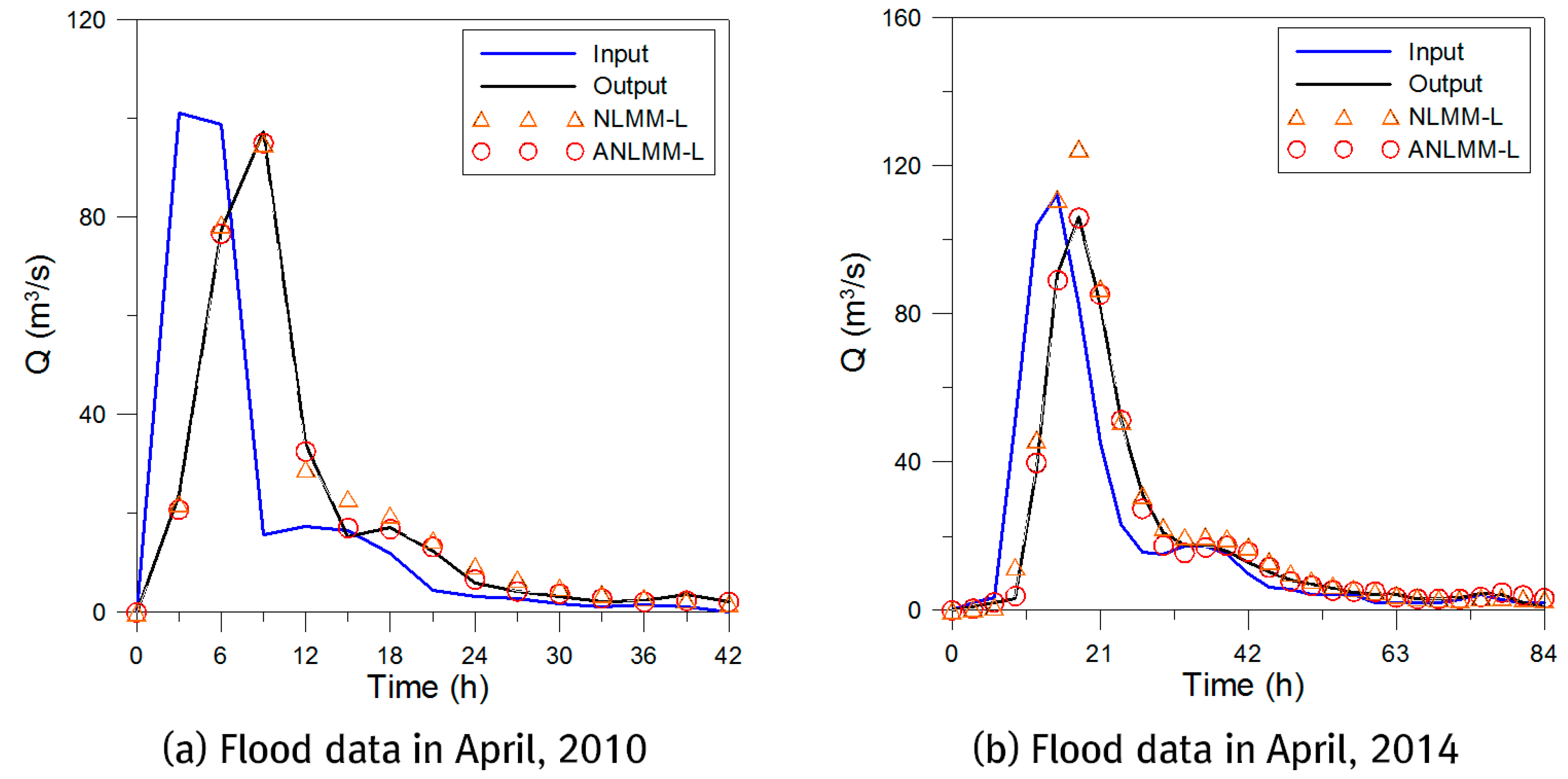
3.6. Application for the Prediction in Daechung Flood Data
4. Discussion
5. Conclusions
Author Contributions
Funding
Acknowledgments
Conflicts of Interest
Abbreviations
| ANLMM-L | Advanced nonlinear Muskingum flood routing model considering continuous flow |
| NLMM-L | Nonlinear Muskingum flood routing model incorporating lateral flow |
| VCA | Vision correction algorithm |
| SSQ | Sum of squares |
| DR1 | Division rate 1 |
| DR2 | Division rate 2 |
| MTF | Modulation transfer function |
| CF | Compression factor |
| AR | Astigmatic rate |
| RMSE | Root mean square error |
| NSE | Nash-Sutcliffe efficiency |
| KWM | Kinematic wave model |
| LMM | Linear Muskingum method |
| LMM-L | Linear Muskingum method incorporating lateral flow |
| NLMM | Nonlinear Muskingum method |
| AF | Astigmatic angle |
| CG | Candidate glasses |
| NFEs | Number of function evaluations |
| CSA | Cuckoo search algorithm |
References
- Jung, C.Y.; Jung, Y.H.; Kim, H.S.; Jung, S.W.; Jung, K.S. The estimation of parameter using Muskingum model in ank-dong river basin incorporating lateral inflow. In Proceedings of the 2008 Korea Water Resources Association Conference, Gyeongju, Korea, 17–18 May 2008. [Google Scholar]
- Kimura, T. The Flood Runoff Analysis Method by the Storage Function Model; The Public Works Research Institute, Ministry of Construction: Tsukuba, Japan, 1961. [Google Scholar]
- McCarthy, G.T. The unit hydrograph and flood routing. In Proceedings of the Conference of North Atlantic Division; US Army Corps of Engineers: Washington, DC, USA, 1938. [Google Scholar]
- O’Donnell, T. A direct three-parameter Muskingum procedure incorporating lateral inflow. Hydrol. Sci. J. 1985, 30, 479–496. [Google Scholar] [CrossRef]
- Tung, Y.K. River flood routing by nonlinear Muskingum method. J. Hydraul. Eng. 1985, 111, 1447–1460. [Google Scholar] [CrossRef]
- Das, A. Parameter estimation for Muskingum models. J. Irrig. Drain. E 2004, 130, 140–147. [Google Scholar] [CrossRef]
- Geem, Z.W. Parameter estimation for the nonlinear Muskingum model using the BFGS technique. J. Irrig. Drain. E 2006, 132, 474–478. [Google Scholar] [CrossRef]
- Karahan, H.; Gurarslan, G.; Geem, Z.W. A new nonlinear Muskingum flood routing model incorporating lateral flow. Eng. Optim. 2015, 47, 737–749. [Google Scholar] [CrossRef]
- Wilson, E.M. Engineering Hydrology; MacMillan Education: Hampshire, UK, 1974. [Google Scholar]
- Wang, W.; Xu, Z.; Qiu, L.; Xu, D. Hybrid chaotic genetic algorithms for optimal parameter estimation of Muskingum flood routing model. In Proceedings of the International Joint Conference on Computational Sciences and Optimization, Sanya, China, 24–26 April 2009; pp. 215–218. [Google Scholar]
- Bajracharya, K.; Barry, D.A. Accuracy criteria for linearised diffusion wave flood routing. J. Hydrol. 1997, 195, 200–217. [Google Scholar] [CrossRef]
- Ulke, A. Flood Routing Using Muskingum Method. Master’s Thesis, Suleyman Demirel University, Kaskelen, Kazakhstan, 2003. (In Turkish). [Google Scholar]
- Karahan, H.; Gurarslan, G. Modelling Flood Routing Problems Using Kinematic Wave Approach: Sutculer Example. In Proceedings of the 7th National Hydrology Congress, Isparta, Turkey, 26–27 September 2013. [Google Scholar]
- Geem, Z.W. Issues in optimal parameter estimation for the nonlinear Muskingum flood routing model. Eng. Optim. 2014, 46, 328–339. [Google Scholar] [CrossRef]
- Todini, E. A mass conservative and water storage consistent variable parameter Muskingum-Cunge approach. Hydrol. Earth Syst. Sci. 2007, 11, 1645–1659. [Google Scholar] [CrossRef]
- Lee, E.H.; Lee, H.M.; Yoo, D.G.; Kim, J.H. Application of a meta-heuristic optimization algorithm motivated by a vision correction procedure for civil engineering problems. KSCE J. Civ. Eng. 2017, 1–14. [Google Scholar] [CrossRef]
- Karahan, H.; Gurarslan, G.; Geem, Z.W. Parameter estimation of the nonlinear Muskingum flood-routing model using a hybrid harmony search algorithm. J. Hydrol. Eng. 2013, 18, 352–360. [Google Scholar] [CrossRef]
- Han River Flood Control Office. Available online: www.hrfco.go.kr (accessed on 30 April 2018).


| Ranges of Parameters in ANLMM-L | K | χ | m | β | θ1 | θ2 |
|---|---|---|---|---|---|---|
| Wilson flood data | 0.01–1.00 | −0.50–0.50 | 1.00–3.00 | −0.10–0.10 | 0.00–1.00 | 0.00–1.00 |
| Flood data by Wang et al. [10] | 0.01–1.00 | −1.50–1.50 | 1.00–3.00 | −3.00–3.00 | 0.00–1.00 | 0.00–1.00 |
| Flood data for River Wye December in 1960 | 0.01–1.00 | −0.50–0.50 | 1.00–3.00 | −0.10–0.10 | 0.00–1.00 | 0.00–1.00 |
| Sutculer flood data | 0.01–1.00 | −0.50–0.50 | 1.00–3.00 | −0.10–0.10 | 0.00–1.00 | 0.00–1.00 |
| Flood data for River Wyre October in 1982 | 0.01–10.00 | −0.50–0.50 | 0.00–1.00 | −3.00–3.00 | 0.00–1.00 | 0.00–1.00 |
| Daechung flood data | 0.01–100.00 | −0.50–0.50 | 1.00–10.00 | −3.00–3.00 | 0.00–1.00 | 0.00–1.00 |
| Objective function f(x), x = (x1, x2, …, xd)T |
| Generate initial glasses |
| While (t < Max number of iterations) |
| if (DR1 < rand) |
| ● Choose an existing glasses/generate new glasses |
| if (DR2 < rand) |
| ● Determine global search direction |
| end |
| end |
| if (new solution < current worst solution) |
| ● Replace new solution with current worst solution |
| end |
| ● Find the current best solution |
| End while |
| Measures | LMM-L | NLMM | NLMM-L | ANLMM-L |
|---|---|---|---|---|
| SSQ | 56 s | 63 s | 64 s | 66 s |
| RMSE | 60 s | 67 s | 68 s | 70 s |
| NSE | 68 s | 70 s | 72 s | 73 s |
| Time (h) | Input (m3/s) | Output (m3/s) | LMM-L (O’Donnell [4]) | NLMM (Karahan [17]) | NLMM-L (Karahan [8]) | ANLMM-L (This Study) |
|---|---|---|---|---|---|---|
| 0 | 22 | 22 | 22 | 22 | 22.00 | 22.00 |
| 6 | 23 | 21 | 22.1 | 22 | 21.71 | 21.57 |
| 12 | 35 | 21 | 21.7 | 22.4 | 22.02 | 21.67 |
| 18 | 71 | 26 | 22.6 | 26.6 | 26.08 | 25.46 |
| 24 | 103 | 34 | 30.7 | 34.5 | 33.51 | 34.59 |
| 30 | 111 | 44 | 44.7 | 44.2 | 42.83 | 43.73 |
| 36 | 109 | 55 | 58.1 | 56.9 | 55.44 | 54.59 |
| 42 | 100 | 66 | 68.9 | 68.1 | 66.67 | 66.01 |
| 48 | 86 | 75 | 76.1 | 77.1 | 75.77 | 75.52 |
| 54 | 71 | 82 | 79.2 | 83.3 | 82.12 | 82.16 |
| 60 | 59 | 85 | 78.5 | 85.9 | 84.78 | 85.04 |
| 66 | 47 | 84 | 75.6 | 84.5 | 83.42 | 84.00 |
| 72 | 39 | 80 | 70.7 | 80.6 | 79.44 | 79.62 |
| 78 | 32 | 73 | 65.1 | 73.7 | 72.48 | 72.63 |
| 84 | 28 | 64 | 59.1 | 65.4 | 64.08 | 63.80 |
| 90 | 24 | 54 | 53.4 | 56 | 54.58 | 54.31 |
| 96 | 22 | 44 | 47.9 | 46.7 | 45.22 | 44.80 |
| 102 | 21 | 36 | 43.1 | 37.7 | 36.34 | 36.25 |
| 108 | 20 | 30 | 38.9 | 30.5 | 29.21 | 29.45 |
| 114 | 19 | 25 | 35.4 | 25.2 | 24.21 | 24.63 |
| 120 | 19 | 22 | 32.3 | 21.7 | 20.96 | 21.39 |
| 126 | 18 | 19 | 29.9 | 20 | 19.41 | 19.81 |
| SSQ | - | - | 815.68 | 36.77 | 9.82 | 4.54 |
| RMSE | - | - | 6.232327 | 1.330234 | 0.683938 | 0.464948 |
| NSE | - | - | 0.965417 | 0.998424 | 0.999584 | 0.999808 |
| Time (12 h) | Input (m3/s) | Output (m3/s) | LMM (Wang et al. [10]) | NLMM (Geem [7]) | NLMM-L (Karahan et al. [8]) | ANLMM-L (This Study) |
|---|---|---|---|---|---|---|
| 1 | 261 | 228 | 228 | 228 | 228.00 | 228.00 |
| 2 | 389 | 300 | 305.19 | 303.8 | 299.74 | 300.92 |
| 3 | 462 | 382 | 382 | 382.3 | 382.57 | 381.51 |
| 4 | 505 | 444 | 442.7 | 442.4 | 442.76 | 443.15 |
| 5 | 525 | 490 | 483.6 | 482.4 | 482.16 | 482.69 |
| 6 | 543 | 513 | 513 | 511.2 | 509.89 | 510.09 |
| 7 | 556 | 528 | 534.29 | 532.3 | 530.72 | 530.66 |
| 8 | 567 | 543 | 550.44 | 548.5 | 546.77 | 546.62 |
| 9 | 577 | 553 | 563.53 | 561.7 | 559.96 | 559.77 |
| 10 | 583 | 564 | 573.16 | 571.6 | 569.94 | 569.80 |
| 11 | 587 | 573 | 580.02 | 578.7 | 577.07 | 576.95 |
| 12 | 595 | 581 | 587.32 | 586.2 | 584.39 | 584.22 |
| 13 | 597 | 588 | 592.14 | 591.2 | 589.68 | 589.60 |
| 14 | 597 | 594 | 594.59 | 593.9 | 592.34 | 592.30 |
| 15 | 589 | 592 | 592.02 | 591.8 | 590.33 | 590.34 |
| 16 | 556 | 584 | 574.89 | 575.7 | 574.68 | 574.86 |
| 17 | 538 | 566 | 556.85 | 558.5 | 556.41 | 556.23 |
| 18 | 516 | 550 | 536.93 | 539 | 537.43 | 537.13 |
| 19 | 486 | 520 | 512.18 | 514.8 | 513.47 | 513.35 |
| 20 | 505 | 504 | 507.96 | 509.6 | 507.07 | 506.51 |
| 21 | 477 | 483 | 493.22 | 494.9 | 494.86 | 494.95 |
| 22 | 429 | 461 | 462.34 | 464.8 | 464.39 | 464.94 |
| 23 | 379 | 420 | 421.87 | 425.1 | 423.97 | 424.15 |
| 24 | 320 | 368 | 372.34 | 376.1 | 375.05 | 375.07 |
| 25 | 263 | 318 | 318.97 | 322.4 | 321.35 | 321.35 |
| 26 | 220 | 271 | 270.39 | 272.5 | 271.42 | 271.40 |
| 27 | 182 | 234 | 226.99 | 227.5 | 226.94 | 227.09 |
| 28 | 167 | 193 | 197.2 | 195.7 | 194.92 | 195.13 |
| 29 | 152 | 178 | 174.87 | 172.6 | 172.46 | 172.76 |
| SSQ | - | - | 1086.84 | 979.96 | 917.06 | 909.35 |
| RMSE | - | - | 6.121869 | 5.820949 | 5.623120 | 5.599733 |
| NSE | - | - | 0.998180 | 0.998354 | 0.998464 | 0.998477 |
| Time (h) | Input (m3/s) | Output (m3/s) | LMM-L (O’Donnell [4]) | NLMM (Karahan et al. [17]) | NLMM-L (Karahan et al. [8]) | ANLMM-L (This Study) |
|---|---|---|---|---|---|---|
| 0 | 154 | 102 | 102 | 154 | 102.00 | 102.00 |
| 6 | 150 | 140 | 116 | 154 | 149.50 | 146.52 |
| 12 | 219 | 169 | 120 | 152 | 156.59 | 155.74 |
| 18 | 182 | 190 | 147 | 181 | 191.40 | 194.41 |
| 24 | 182 | 209 | 158 | 191 | 200.79 | 194.19 |
| 30 | 192 | 218 | 165 | 185 | 195.14 | 196.05 |
| 36 | 165 | 210 | 176 | 187 | 197.46 | 198.35 |
| 42 | 150 | 194 | 178 | 179 | 188.48 | 186.83 |
| 48 | 128 | 172 | 176 | 162 | 170.80 | 172.12 |
| 54 | 168 | 149 | 164 | 141 | 148.10 | 150.37 |
| 60 | 260 | 136 | 160 | 154 | 162.59 | 167.56 |
| 66 | 471 | 228 | 167 | 198 | 210.36 | 216.61 |
| 72 | 717 | 303 | 218 | 264 | 281.58 | 294.27 |
| 78 | 1092 | 366 | 303 | 344 | 367.75 | 378.29 |
| 84 | 1145 | 456 | 484 | 416 | 447.65 | 461.17 |
| 90 | 600 | 615 | 690 | 599 | 629.57 | 612.03 |
| 96 | 365 | 830 | 700 | 871 | 892.78 | 862.51 |
| 102 | 277 | 969 | 642 | 834 | 859.01 | 884.60 |
| 108 | 227 | 665 | 572 | 689 | 719.30 | 737.54 |
| 114 | 187 | 519 | 505 | 535 | 567.50 | 565.33 |
| 120 | 161 | 444 | 442 | 397 | 427.85 | 414.97 |
| 126 | 143 | 321 | 386 | 283 | 308.86 | 297.45 |
| 132 | 126 | 208 | 338 | 202 | 220.90 | 216.14 |
| 138 | 115 | 176 | 296 | 152 | 163.64 | 164.43 |
| 144 | 102 | 148 | 260 | 124 | 131.90 | 134.94 |
| 150 | 93 | 125 | 228 | 106 | 111.93 | 114.46 |
| 156 | 88 | 114 | 201 | 94 | 99.28 | 101.24 |
| 162 | 82 | 106 | 179 | 88 | 92.90 | 94.00 |
| 168 | 76 | 97 | 160 | 82 | 86.14 | 86.94 |
| 174 | 73 | 89 | 144 | 75 | 79.34 | 80.13 |
| 180 | 70 | 81 | 130 | 73 | 76.46 | 76.87 |
| 186 | 67 | 76 | 118 | 69 | 73.13 | 73.54 |
| 192 | 63 | 71 | 109 | 66 | 69.85 | 70.23 |
| 198 | 59 | 66 | 100 | 62 | 65.09 | 65.60 |
| SSQ | - | - | 251,802 | 37,944.15 | 25,915.27 | 20,494.98 |
| RMSE | - | - | 87.351953 | 33.900478 | 28.023846 | 24.921077 |
| NSE | - | - | 0.892983 | 0.983882 | 0.988986 | 0.991290 |
| Time (h) | Input (m3/s) | Output (m3/s) | KWM (Karahan and Gurarslan [13]) | NLMM-L (Karahan et al. [8]) | ANLMM-L (This Study) |
|---|---|---|---|---|---|
| 0 | 7.53 | 7 | 7.00 | 7.00 | 7.00 |
| 1 | 9.06 | 8 | 7.62 | 7.24 | 7.26 |
| 2 | 28 | 23 | 9.98 | 9.00 | 9.01 |
| 3 | 79.8 | 25 | 29.16 | 27.35 | 27.35 |
| 4 | 64.3 | 75 | 73.78 | 74.84 | 74.81 |
| 5 | 38.2 | 60 | 63.01 | 61.57 | 61.59 |
| 6 | 41.4 | 40 | 41.98 | 37.40 | 37.41 |
| 7 | 41.3 | 41 | 41.25 | 39.63 | 39.62 |
| 8 | 33.8 | 41 | 40.48 | 39.47 | 39.47 |
| 9 | 32 | 32 | 34.64 | 32.57 | 32.58 |
| 10 | 29 | 30 | 32.13 | 30.68 | 30.68 |
| 11 | 35 | 34 | 29.52 | 28.00 | 28.00 |
| 12 | 63.1 | 35 | 36.16 | 33.93 | 33.93 |
| 13 | 110 | 60 | 62.98 | 60.62 | 60.62 |
| 14 | 170 | 105 | 108.45 | 105.25 | 105.25 |
| 15 | 216 | 160 | 166.29 | 162.06 | 162.07 |
| 16 | 131 | 206 | 206.02 | 204.11 | 204.11 |
| 17 | 101 | 128 | 136.31 | 127.58 | 127.61 |
| 18 | 65 | 97 | 104.68 | 97.14 | 97.10 |
| 19 | 62.4 | 61 | 67.14 | 63.33 | 63.32 |
| 20 | 53.8 | 60 | 63.35 | 59.78 | 59.76 |
| 21 | 36.3 | 50 | 53.18 | 51.51 | 51.50 |
| 22 | 29.6 | 33 | 37.84 | 35.16 | 35.16 |
| 23 | 25 | 27 | 30.34 | 28.49 | 28.48 |
| 24 | 21.3 | 23 | 25.11 | 24.03 | 24.03 |
| 25 | 19.6 | 19 | 21.68 | 20.49 | 20.49 |
| 26 | 18 | 18 | 19.71 | 18.81 | 18.81 |
| 27 | 17.3 | 17 | 18.1 | 17.29 | 17.29 |
| 28 | 17 | 17 | 17.39 | 16.60 | 16.60 |
| 29 | 16 | 17 | 16.97 | 16.29 | 16.29 |
| SSQ | - | - | 532.62 | 281.11 | 280.95 |
| RMSE | - | - | 4.213541 | 3.062067 | 3.060222 |
| NSE | - | - | 0.992271 | 0.995918 | 0.995923 |
| Time (h) | Input (m3/s) | Output (m3/s) | LMM-L (O’Donnell [4]) | NLMM-L (Karahan et al. [8]) | ANLMM-L (This Study) |
|---|---|---|---|---|---|
| 0 | 2.6 | 8.3 | 8.3 | 8.3 | 8.30 |
| 1 | 4.2 | 9 | 8.2 | 8.51 | 8.52 |
| 2 | 12.3 | 9.9 | 8.1 | 8.79 | 9.94 |
| 3 | 25.4 | 10.2 | 12.7 | 10.94 | 12.74 |
| 4 | 24.1 | 18.9 | 27.9 | 20.28 | 19.71 |
| 5 | 20.3 | 35.9 | 39.9 | 37.54 | 35.73 |
| 6 | 23.3 | 51.8 | 45.7 | 49.07 | 48.87 |
| 7 | 27.7 | 59.4 | 52.2 | 55.11 | 55.95 |
| 8 | 27.7 | 63.3 | 61.4 | 62.5 | 62.74 |
| 9 | 26.9 | 69.6 | 68.9 | 71.44 | 71.35 |
| 10 | 24.8 | 76.7 | 74.7 | 78.03 | 77.95 |
| 11 | 26.9 | 82 | 77.2 | 82.07 | 82.67 |
| 12 | 33.7 | 85.3 | 79.8 | 83.72 | 85.27 |
| 13 | 33.9 | 89 | 87.8 | 87.43 | 88.11 |
| 14 | 27.8 | 94.6 | 95.5 | 95.49 | 94.74 |
| 15 | 20.8 | 98.8 | 97.7 | 100.88 | 99.90 |
| 16 | 15.6 | 98 | 94.4 | 99.29 | 98.87 |
| 17 | 11.9 | 91.8 | 87.9 | 92.06 | 92.05 |
| 18 | 9.5 | 82.3 | 79.8 | 82.22 | 82.36 |
| 19 | 7.8 | 72 | 71.5 | 71.75 | 71.88 |
| 20 | 6.5 | 61.9 | 63.6 | 61.94 | 61.93 |
| 21 | 5.8 | 53 | 56.1 | 53.12 | 53.10 |
| 22 | 5.0 | 45.6 | 49.6 | 45.47 | 45.37 |
| 23 | 4.8 | 39.2 | 43.7 | 39.14 | 39.04 |
| 24 | 4.5 | 33.8 | 38.8 | 33.76 | 33.65 |
| 25 | 4.1 | 29.3 | 34.6 | 29.55 | 29.39 |
| 26 | 3.7 | 26.2 | 30.9 | 26.12 | 25.96 |
| 27 | 3.4 | 23.5 | 27.7 | 23.2 | 23.08 |
| 28 | 3.2 | 21.2 | 24.8 | 20.67 | 20.59 |
| 29 | 2.9 | 19.2 | 22.3 | 18.52 | 18.44 |
| 30 | 2.8 | 17.7 | 20.1 | 16.71 | 16.68 |
| 31 | 2.6 | 16.4 | 18.2 | 15.12 | 15.09 |
| SSQ | - | - | 468.84 | 53.66 | 40.16 |
| RMSE | - | - | 3.790780 | 1.263563 | 1.120320 |
| NSE | - | - | 0.989570 | 0.998842 | 0.999090 |
© 2018 by the authors. Licensee MDPI, Basel, Switzerland. This article is an open access article distributed under the terms and conditions of the Creative Commons Attribution (CC BY) license (http://creativecommons.org/licenses/by/4.0/).
Share and Cite
Lee, E.H.; Lee, H.M.; Kim, J.H. Development and Application of Advanced Muskingum Flood Routing Model Considering Continuous Flow. Water 2018, 10, 760. https://doi.org/10.3390/w10060760
Lee EH, Lee HM, Kim JH. Development and Application of Advanced Muskingum Flood Routing Model Considering Continuous Flow. Water. 2018; 10(6):760. https://doi.org/10.3390/w10060760
Chicago/Turabian StyleLee, Eui Hoon, Ho Min Lee, and Joong Hoon Kim. 2018. "Development and Application of Advanced Muskingum Flood Routing Model Considering Continuous Flow" Water 10, no. 6: 760. https://doi.org/10.3390/w10060760
APA StyleLee, E. H., Lee, H. M., & Kim, J. H. (2018). Development and Application of Advanced Muskingum Flood Routing Model Considering Continuous Flow. Water, 10(6), 760. https://doi.org/10.3390/w10060760