Article

Modeling the Pyrolysis and Combustion Behaviors of Non-Charring and Intumescent-Protected Polymers Using “FiresCone”

1
Centre for Environmental Safety and Risk Engineering, Victoria University, VIC 3030, Australia
2
Department of Building, National University of Singapore, Singapore 117566, Singapore
*
Author to whom correspondence should be addressed.
Polymers 2015, 7(10), 1979-1997; https://doi.org/10.3390/polym7101495
Submission received: 19 August 2015 / Revised: 18 September 2015 / Accepted: 25 September 2015 / Published: 13 October 2015

Abstract

:
A mathematical model, named FiresCone, was developed to simulate the pyrolysis and combustion processes of different types of combustible materials, which also took into account both gas and solid phases. In the present study, some non-charring and intumescent-protected polymer samples were investigated regarding their combustion behaviors in response to pre-determined external heat fluxes. The modeling results were validated against the experimental outcomes obtained from a cone calorimeter. The predicted mass loss rates of the samples were found to fit reasonably well with the experimental data collected under various levels of external irradiation. Both the experimental and modeling results showed that the peak mass loss rate of the non-charring polymer material occurred near the end of burning, whereas for the intumescent-protected polymer it happed shortly after the start of the experiment. “FiresCone” is expected to act as a practical tool for the investigation of fire behavior of combustible materials. It is also expected to model fire scenarios under complicated conditions.

Graphical Abstract

1. Introduction

The extensive use of polymeric materials in our daily life can be attributed to their versatile properties, such as the easiness to process and their light weight. However, polymers are known for their relative high flammability attribute and tendency to produce toxic gases, as compared to their counter parts, upon combustion [1]. Intumescent polymers are a class of materials that have been increasingly used in construction, transportation, manufacturing, etc., primarily owing to their superior fire performance. Non-charring polymers, on the other hand, are significantly flammable and generally transform into gaseous volatile species almost completely during pyrolysis reactions, thus leaving no or little residue [2]. Intumescent polymers, in contrast, are capable of forming substantial amounts of carbonaceous residue, which in turn protects the surface of polymers that are being exposed to an external heat flux [3]. The carbon-rich char residue, initially formed, can undergo rapid expansion primarily owing to the production of non-combustible gaseous species emanating from the decomposing spumific agent within the intumescent formulation.
A large number of pyrolysis models have been developed in the past to simulate the behaviors of combustible materials under a variety of fire conditions. A recent review by Shi and Chew [4] showed that most of the previous models have concentrated on wood, and that only relatively fewer numbers have focused on non-charring and intumescent polymers. After reviewing the solution of the solid and gas phase combustion of solid fuels, Karim and Naser [5] concluded that the numerical modeling of the solid phase remains a challenge for researchers due to complex mechanisms and experimental limitations. A comprehensive computational fluid dynamics (CFD) model of wood combustion have also been developed by Novozhilov et al. [6], where the thermal degradation of two solid materials, such as particle board and Pacific maple, when subjected to a constant radiant heat flux, were considered. This study also highlighted the need to obtain the thermo-physical data for the materials of interest if the details of the mass-loss rate were to be evaluated. Di Blasi and his colleagues also performed a great deal of modeling attempts on wood [7,8], and on other charring polymers [9] as well on non-charring polymers [10]. Recently, many comprehensive pyrolysis models have gained prominence as they have greater flexibility in descripting the pyrolysis of a solid mathematically, as compared to the simpler pyrolysis models that were suggested previously [11]. Lautenberger et al. [12,13] have developed a generalized model, named “Gpyro”, to simulate the fire behavior of non-charring polymers, other charring solids and intumescent coatings. Stoliarov et al. [14,15,16] have also developed a model, named “ThermaKin”, with a view to describing the pyrolysis of solid materials that were exposed to an external heat flux.
In spite of the wealth of information regarding the modeling attempts found in the literature, a systematic and comprehensive attempt to describing the gas phase is still found elusive. In fact, only very few models were reported previously regarding the gas phase modeling. Therefore, it is challenging to develop a model that can describe burning of combustible materials by considering both gas and solid phases [4] and one that yields a good agreement with experimental data. The previous studies also showed that differences, of varying degrees, exist between the modeling outcomes and experimental results, as is evident from the following reports. Riccio et al. [17] have developed a numerical model to simulate the behavior of composite materials in a fire environment providing the mass loss rate, heat release rate and total heat released through the influence of a heat source. Marquis et al. [18] have also developed a model describing the de-volatilization processes of a sandwich material on smaller scale. Yuen et al. [19] have developed a mathematical model for describing the pyrolysis of wet wood that coupled the gas phase combustion to the analyses of a wood samples ignited in a cone calorimeter.
Generally, to improve the modeling accuracy, several additional considerations need to be taken into account, such as the melting process of polymeric material and internal gas pressure. An accurate representation of some phase changes, such as melting and evaporation, is also important to improve the validity of the model. For example, noticeable amounts of volatiles are often found to exhaust from melted polymer matrix under thermal irradiance even though it is not easily observable under ambient conditions. This phenomenon is usually taken into account in the course of the development of a model, where mobile phases due to the melted polymer and/or the formation of porous char layers are also considered. Here the internal gas pressure, which is crucial to describing the transportation of liquid and gaseous species within the solid phase, is also affected by its permeability and porosity. Moreover, the development of a numerical model is also challenging, as there is no common agreement by the various researchers on the relative importance of the various physio-chemical processes that accompany the combustion of solid fuels. For example, many models have considered volume change under external heat flux; however, no common agreement exists about its description or influence, as described in the literature between the different authors [20,21,22,23,24].
Some of the important processes considered in “FiresCone” [25] include melting and evaporation, and the effect of internal pressure build-up on the transportation of the volatiles. These processes have not been previously considered in detail at all; or where considered, have not been done simultaneously, and therefore, their interaction has not been understood previously. Furthermore, some of the models do not consider the gas phase (diffusion flame modeling) [8,13,26]. In the present paper, we wish to report on extended experimental validation of the models against the full combustion history of burning samples, including ignition, burning and extinction. In comparison, the experimental data used for validation in previous studies was limited, as it did not consider material extinction (full fuel consumption) conditions. Therefore, a non-charring and an intumescent-protected polymer samples are considered for modeling and experimental validation purposes, namely, polymethyl methacrylate (PMMA, non-charring) and polycarbonate (PC, intumescent polymer). These samples were obtained, in the form of slabs, from local company in Singapore.

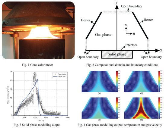
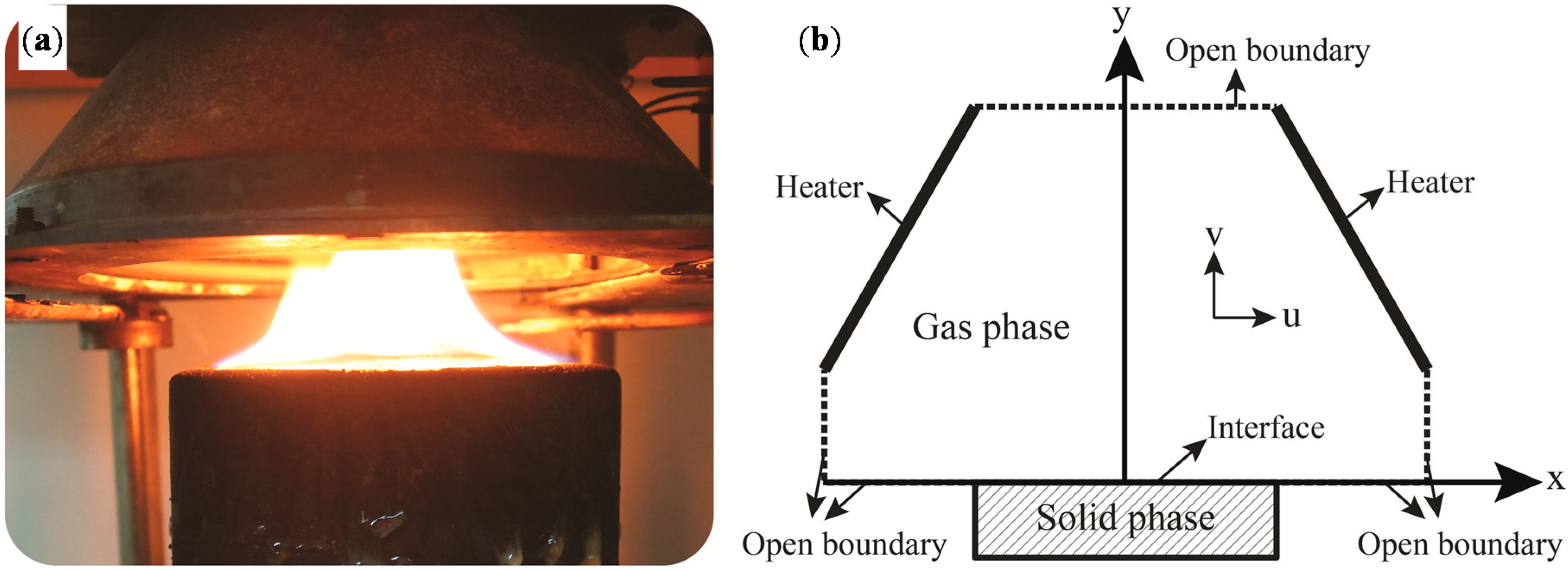
2. Experimental Methodology

The image on the left part in Figure 1 shows the experimental set-up under a cone calorimeter, which is a standard apparatus to test piloted and auto-ignition of solid materials (ISO 5660 [27]). The cone calorimeter was placed under a bigger hood within an exhaust system (extraction rate of 24 L/s). This extraction induces a forced convection driven flow at the top boundary. Samples were placed on to a specimen holder in a horizontal configuration. External heat fluxes of 25, 50 and 75 kW/m2 represent the low, middle and high heat fluxes under fire conditions in an enclosure, respectively. Furthermore, the two sample thicknesses (i.e., 10 and 20 mm) were chosen by following the dimensions of common building components. Before the experimental runs, gas analyzers and the level of external radiant flux were calibrated by using standard means. Table 1 shows a list of experimental and numerical design and parameters.
Figure 1. Cone calorimeter: (a) experimental setup; and (b) computational domain of FiresCone.
Polymers 07 01495 g001
Table 1. A list of experimental and numerical design and parameters.
ItemDescriptionThickness (mm)Heat flux (kW/m2)Formula
MaterialPMMA10, 2025, 50, 75–C5H8O2
PC10, 2025, 50, 75–C16H14O3
Computational domainGas phaseWidth 80 mm
Height 100 mm
Solid phaseDepend on sample thickness
The edges and rear surface of samples were covered with an aluminum foil, and ceramic fiber blanket was inserted underneath a sample for the purpose of insulation, and therefore to ensure minimum heat losses from the sample while undergoing combustion. Samples were then secured on to the specimen holder and placed under the cone heater. The changes in the sample’s weight were continuously recorded using a built-in weighing device. Auto-ignition of the samples was affected in the absence of a piolet, and the onset was taken as the first appearance of visible plumes. Each experiment was repeated at least two times, and optionally more runs were undertaken to ensure an acceptable level of reproducibility. Further details of the experimental runs are published elsewhere [28].

3. Mathematical Model

3.1. Major Assumptions

A mathematical model, “FiresCone”, was developed to simulate the fire behaviors of combustible materials under external heat flux considering both the solid and gas phases. To improve the modeling accuracy, fire processes such as water evaporation, volume change, liquids and gases transportation and in-depth radiation were considered. Three types of reactions were considered in “FiresCone”. The first is to describe physical change, such as water evaporation and melting of polymers. The Arrhenius model was used to describe physical change rate. The second kind of reaction is heterogeneous reaction, which describes the reaction with more than one phase, and the last type of reactions is homogenous reaction. As the thermal properties of each grid in the solid phase are related to the mass and volume, thermal properties in the solid phase were estimated in two ways, such as on mass fraction basis and volume fraction basis.
Both the solid and gas phases are considered in “FiresCone”. Several assumptions are also adopted here: (i) The computational domain was divided into the solid and gas phases—the solid phase is considered as one-dimensional, and the gas phase as two-dimensional. First of these assumptions is consistent with the predominant (normal) direction of heat transfer in the material, which conforms to the experimental observation. During the cone calorimeter tests, the edges and bottom of the samples were covered by insulation materials, which in effect simplify the situation to a one dimensional heat transfer problem, as the heat energy is assumed to travel through the material in the downward direction only. The second assumption means that a round cone under the symmetry is approximated, for simplicity, by a square one with an equivalent cross-sectional area; (ii) Homogeneous reactions in the solid phase are ignored because of their less likelihood to produce gaseous products as compared to those during the pyrolysis reaction of solid fuels, and therefore are only considered in the gas phase. This is due to the fact that the amount of volatiles produced, if at all, is much smaller than those during the main pyrolysis reaction of solid fuels; (iii) All the gas species are considered to have the same thermal properties, as the difference in the properties between each species is small, thus resulting in small difference in the output. Gas species in the solid phase are assumed to be ideal gases, and the gas species in the gas phase are treated as incompressible ideal gases; (iv) The influence of volume change in the solid phase on the gas phase was ignored; (v) Failure processes, such as cracking, are ignored owing to the complexity of the situation; and (vi) The thermal feedback from flame to burning material is assumed to be negligible as compared with the external radiation.

3.2. The Governing Equations

3.2.1. The Solid Phase

A schematic sketch of a computational domain, which corresponded to the experimental set-up, is shown in the right hand side of Figure 1. For a comprehensive description of our model please refer to the previous work [25]. The physical and chemical processes that are being modeled are: (i) thermal decomposition (pyrolysis) of solid species; and (ii) vaporization of water from the matrix of solid material. Both mechanistic pathways (i) and (ii) result in production of gaseous products that are considered to be subsequently transported through the porous matrix towards exposed surface of the sample. The description of gas transportation inside the samples was assumed to obey the Darcy’s law considering the porous nature of the matrix.
Given that the material under consideration can be multi-component and that it is very difficult to completely quantify all the gases emanating from it upon degradation, the evaluation of the exact pyrolysis kinetics practical can be rather complicated. No intermediate species are also considered because of the fact that those products were obtained from experiments that showed the user-specified gas yields, which represented the amount of gas produced after burning the specific solid fuels. Therefore in the present study, the decomposition is modeled by chemical reactions of the form:
v 1 s j [ S ] 1 s j + v 1 g j [ G ] 1 g j               k j                   v 2 s j [ S ] 2 s j + v 2 g j [ G ] 2 g j + Δ h j
The above scheme is written on a mass basis, with the kinetic parameters evaluated from available data [29,30,31,32]. Here [S] stands for solid species and [G] stands for gas species.
Conservation equations of the solid phase are expressed as:
i = 1 N s + N l + N g ρ i ϕ C p , i T s t + j = 1 N l + N g ρ j ϕ C p , j T s u j x = x ( λ T s x ) + Q p y r + q ˙ r a d " x
ρ i t = Θ i
ρ g ϕ t + ρ g ϕ u x = ( Θ i + Θ l )
ρ l t + ρ l u x = Θ l
Here, Equation (2) is the energy conservation equation; Equation (3) describes the consumption of solid species; and Equations (4) and (5) are mass conservations for gas and liquid, respectively. Note here that the densities are defined by averaging over the local volume of the solid material; therefore, for instance, the liquid density is taken to vary with space/time.
Equations (2)–(5) are supplemented by the constitutive relations (Darcy’s law) applying to both gas and liquid flows through the porous matrix of the material:
u g = γ g μ g ϕ P x , u l = γ l μ l P x
Reaction terms are modeled as:
Θ i = j v 1 s j k j ρ j n j , k j = A j exp ( E j R T ) , Θ l = A l exp ( E l R T ) ρ l
The Arrhenius kinetics treatment in Equation (7) is justified in the case of water, embedded as moisture into the porous matrix of the material and effectively without free surface [33].
Heat of reaction is the change in enthalpy when one material changes to another during a reaction. The enthalpy change of reaction can be obtained by standard enthalpy of formation of the reactants and products, such as in homogeneous and heterogeneous reactions [34]. The heat generated or absorbed by pyrolysis reactions is described as:
Q p y r = j Δ h j k j
Radiation heat transfer is an important phenomenon in combustion modeling, considering the emissivity [35]. Beer–Lambert Law states that there is a logarithmic dependence between transmission of light through a substance and the absorption coefficient of this substance multiplied by the distance the light travel through the substance (i.e., the path length). The absorption of radiation is assumed to follow the Beer–Lambert’s law, i.e., the radiation heat flux diminishes away from the exposed surface as:
q ˙ r a d = q ˙ e x t exp ( κ x )

3.2.2. The Gas Phase

Two-dimensional Navier–Stokes equations, supplemented with the continuity, energy and species conservation equations are adopted for the gas phase, as follows:
ρ C p T t + ρ C p u T x + ρ C p v T y = x ( λ T x ) + y ( λ T y ) + Q r e a c
u x + v y = 0
ρ u t + ρ u u x + ρ v u y = x ( μ u x ) + y ( μ u y ) P x
ρ v t + ρ u v x + ρ v v y = x ( μ v x ) + y ( μ v y ) P y
ρ Y i t + ρ u Y i x + ρ v Y i y = x ( ρ D Y i x ) + y ( ρ D Y i y ) + Θ r e a c
In the absence of detailed information on the chemical composition of pyrolysis products (which is quite complex and difficult to quantify precisely), the following simplified treatment is implemented.
The chemical reaction in the diffusion flame is written in a general form on a mass basis as
[ F ] + ν O 2 [ O 2 ]    k f    ν C O [ C O ] + ν C O 2 [ C O 2 ] + ν H 2 O [ H 2 O ] + Δ h f
Here the reaction rate constant and the rate of heat release given by:
k f = A f exp ( E f R T ) , Q r e a c = k f ρ 2 Y F Y O 2 Δ h f
Relevant stoichiometric and kinetic parameters are listed in Table 2 and Table 3.
During the simulation, the top boundary conditions are set in terms of exit velocity of the gas leaving the heater. This velocity is determined by the volumetric extraction rate (24 L/s) through the hood that encloses the cone heater. The bottom and side open boundaries were considered as open boundaries, and no-slip conditions are imposed on the solid boundaries (walls).

3.3. The Numerical Approach

The governing equations were solved through a fully implicit Finite Volume Method. Staggered grids were used to avoid convergence problems and oscillations in the pressure field. Quadratic Upstream Interpolation for Convective Kinematics (QUICK) is a high order differencing scheme, which was used to discretize all convective terms, as it includes the information of three control volumes from upstream. Pressure Implicit with Splitting of Operators (PISO) was used to solve the coupled pressure–velocity problem.
For the solid phase, sensitivity analysis showed that the grid spacing has limited influence on the surface temperature and mass loss rate when grid spacing is less than 0.1 mm. For the gas phase, grid spacing of 2 and 4 mm were used for sensitivity analysis. The calculation time increased significantly when the grid spacing was reduced from 4 to 2 mm. A comparison of results with these two grid sizes over the first 50 s of calculations showed little difference. Therefore, grid sizes of 4 mm × 4 mm were used in the solid and gas phases, respectively. The total number of control volumes is 42 × 27, in X and Y directions in the gas phase, respectively. The one-dimensional solid phase simulation required approximately 0.5–3 h of CPU time on a single core of 2.3 GHz processor, and the two-dimensional simulations of the gas phase combustion required more than 10 h, depending on the time of sample burning.

4. Results and Discussion

4.1. Non-Charring Polymer

4.1.1. Thermal Properties of PMMA

Table 2 shows the thermal properties of PMMA for the modeling input. PMMA is a typical non-charring polymer, and it burns out without leaving any residue. It should be noted here that it becomes impossible to continue with the modeling when the size of some grids become zero as all the PMMA matrix changes into gaseous volatiles. Therefore, in “FiresCone”, in order to avoid empty grids, it was assumed that there are only very few char residues left after the burning of PMMA samples under the different heating regimes. As liquid water content inside polymer is very low [36], its presence if at all can be ignored. The reactions considered in the numerical model were:
P M M A       b P M M A
P M M A       F u e l + C h a r ( v e r y l i t t l e )
b P M M A       F u e l + C h a r ( v e r y l i t t l e )
Here bPMMA is bubbled PMMA, representing the melted PMMA; the char yield was assumed to be very little in the numerical modeling in order to avoid an empty grid, as previously mentioned.
Table 2. The thermal properties of PMMA taken as the input for modeling.
PropertyUnitPMMAbPMMAChar (nominal)Gas
Pyrolysis reaction rate1/s 8.5 × 10 12 e 188000 R T [15] 8.5 × 10 12 e 188000 R T [15]--
Melting rate1/s 2.9 × 10 47 e 366250 R T [2]---
Densitykg/m31,202.9 [27]1,000.01,202.91.205
Heat of pyrolysiskJ/kg1,3501,350--
Gas permeabilitym25.80 × 10−165.80 × 10−165.80 × 10⁻¹⁶-
Water permeabilitym23.79 × 10−193.79 × 10−193.79 × 10⁻¹⁹-
Diffusion coefficient of waterm2/s5.11 × 10−85.11 × 10−85.11 × 10−8-
Diffusion coefficient of gasm2/s1.85 × 10−91.85 × 10−91.85 × 10−9-
Specific heat capacityJ/kg·K1,500 [37]2,200 [37]2,2001,000 [38]
Surface emissivity-0.96 [39]0.96 [39]0.96-
Thermal conductivityW/m·K0.16 [37]0.21 [37]0.210.03 [40]
Absorption coefficient1/m960 [39]960 [39]0.1-
Dynamic viscosityPa·s---2.0 × 10⁻⁵ [41]
Generally, it is considered to be somewhat difficult for gases and liquids to pass through PMMA slab. However, gaseous species are assumed to percolate into the ambient atmosphere through the bPMMA, which may be similar to the process occurring in liquid water, at least in some respects. No data has been found about the permeability and diffusion coefficient of gaseous species that are of interest to us, through virgin PMMA or bPMMA. Therefore, these values were assumed to be same as those for the liquid water, albeit the fact that this assumption is only a gross approximation. As the empty grids, after the burning out of bPMMA, was also assumed to be filled by air (as in the case of the actual experimental runs), and therefore the absorption coefficient of char in the modeling attempt was assumed to be equal to that of air. Other properties of char in modeling were taken as the same as that of bPMMA, as in actual practice, virtually no char residue is left after its complete combustion.

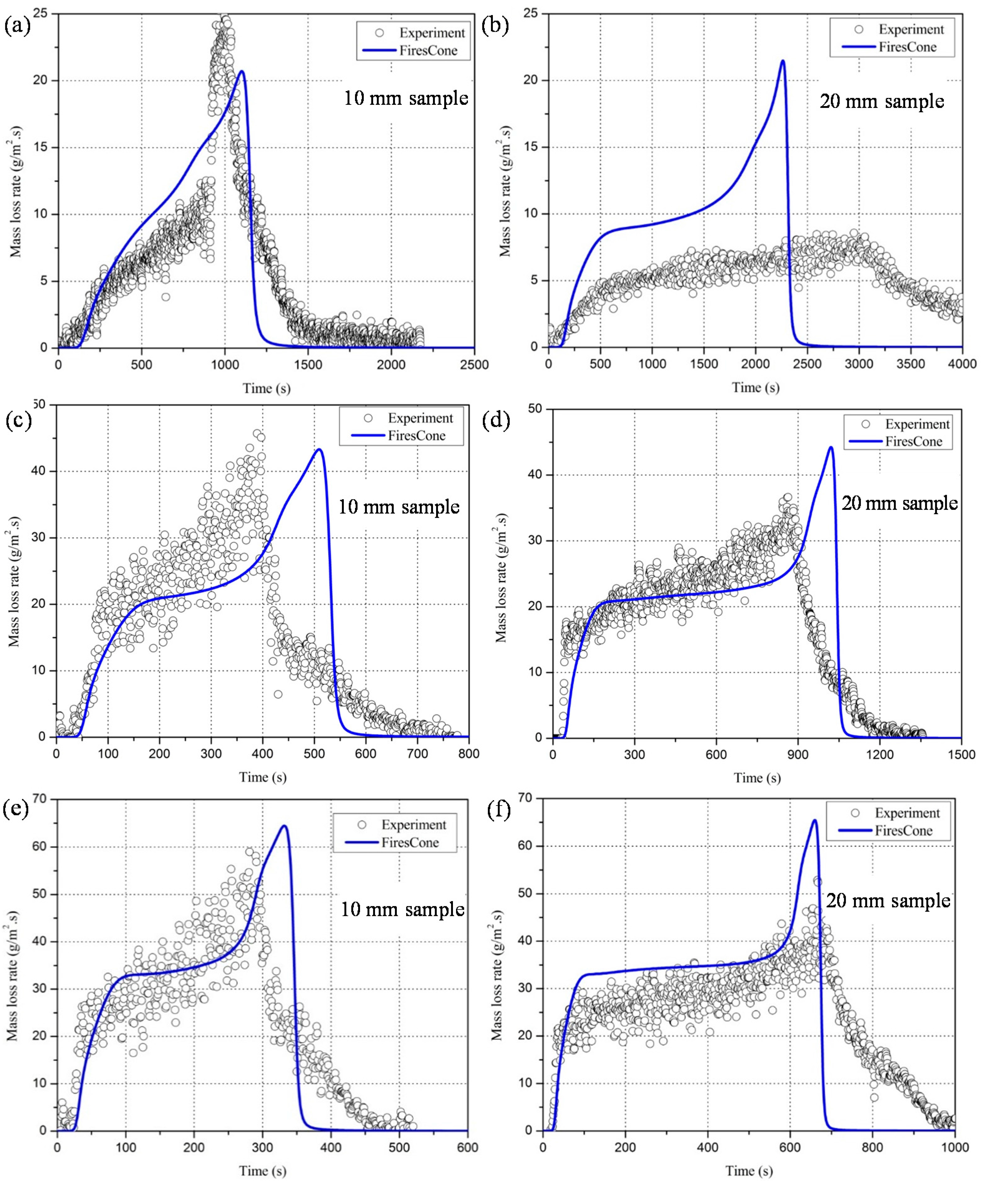
4.1.2. Mass Loss Rate

Figure 2a,b show a comparison of the mass loss rate (MLR) between modeling and experiments for PMMA samples, of 10 and 20 mm thicknesses, under 25 kW/m2 of heat flux. It can be seen that the modeling results agree well with experiments for the 10 mm thick sample. However, the modeling results for 20 mm thickness of PMMA show much higher MLR than the experiment. This can be attributed to the fact that the 20 mm thick sample did not undergo flaming combustion at all—it only underwent melting and the exclusion of some dissolved air, and perhaps some low molecular weight volatile fragments, thus showing a very low MLR. This might indicate that the critical heat flux for PMMA is above 25 kW/m2 under the auto-ignition regime.
Figure 2. Comparisons between modeling and experimental results for PMMA under different heat fluxes: (a,b) 25 kW/m2; (c,d) 50 kW/m2; and (e,f) 75 kW/m2.
Polymers 07 01495 g002
The mass loss rate curves of PMMA under 50 kW/m2 of heat flux can be seen in Figure 2c,d. As can be seen, the modeling results agree well with the experimental ones. It is relevant to note here that, in a previous report, Tewarson [42] has configured the entire burning of a typical non-charring polymer into three stages: solid, molten and boiling liquid stages. It was also observed that peak HRR (or the corresponding peak MLR) occurred in the last stage of the cone run. This can be attributed to the thermal feedback that occurs when pyrolysis zone reaches the bottom part of the sample. It is also known that, generally, the modeling results clearly shows all the three stages: firstly, the MLR increases fast just after ignition; in the second stage, the entire PMMA matrix start to melt when temperature rises, and the MLR increases smoothly; and, in the last stage, all the solid material changes into liquid, and the peak MLR appears in this “liquid boiling stage” owing to feedback of heat energy from the insulated bottom.
From Figure 2c,d, it is observed that trend of MLR in the first and the third stages are similar for two samples with different thicknesses. Influence of thickness on MLR is also reflected by the prolonged period for the second stage, namely molten stage. For instance, the second stage for the 10 mm thickness PMMA lasts less than 300 s, but for 20 mm thickness PMMA it is longer than 600 s.
Figure 2e,f show MLR of PMMA under 75 kW/m2 heat flux. It can be also observed that the results from the modeling closely follow that from the experiments. Furthermore, all the expected stages can be easily identified, from both the modeling and experimental results, and the peak of the MLR is seen to appear during the final stages of the combustion of the samples. The predicted MLR at the end is much lower than the experiments, which is probably because of the absence of accurate empirical model to describe the melting process of PMMA. The prediction can be improved after these kinds of data are available.

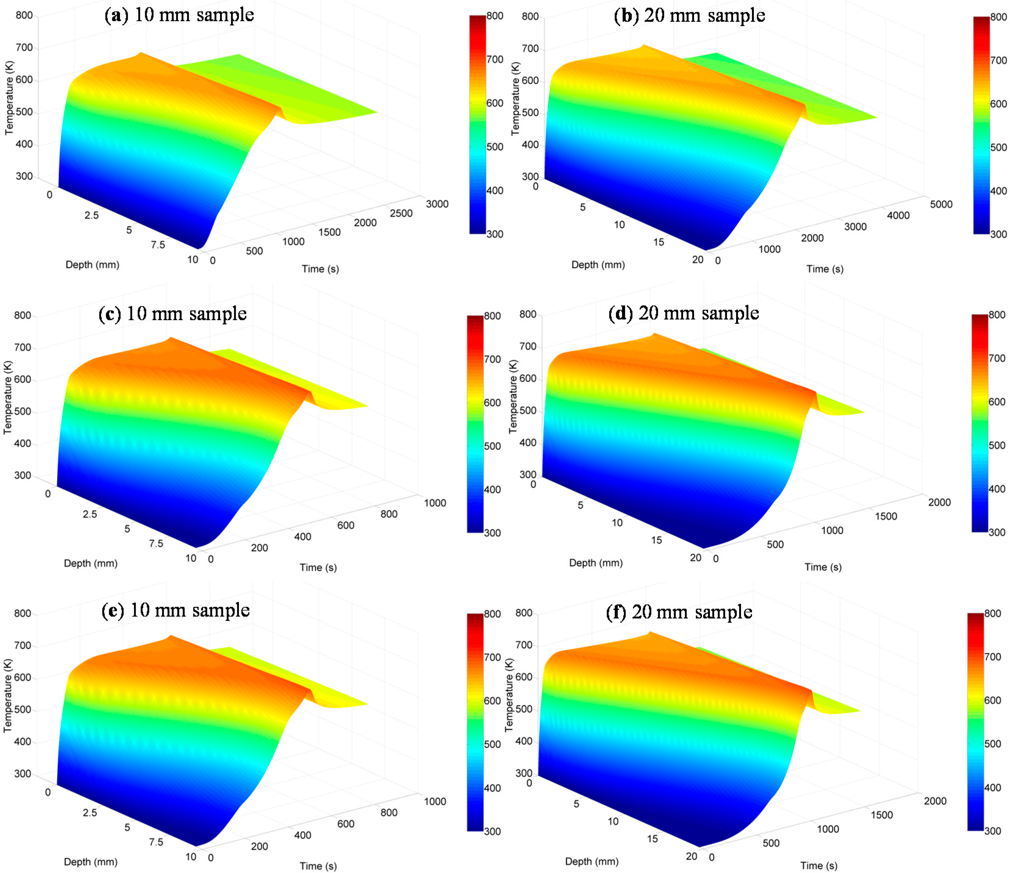
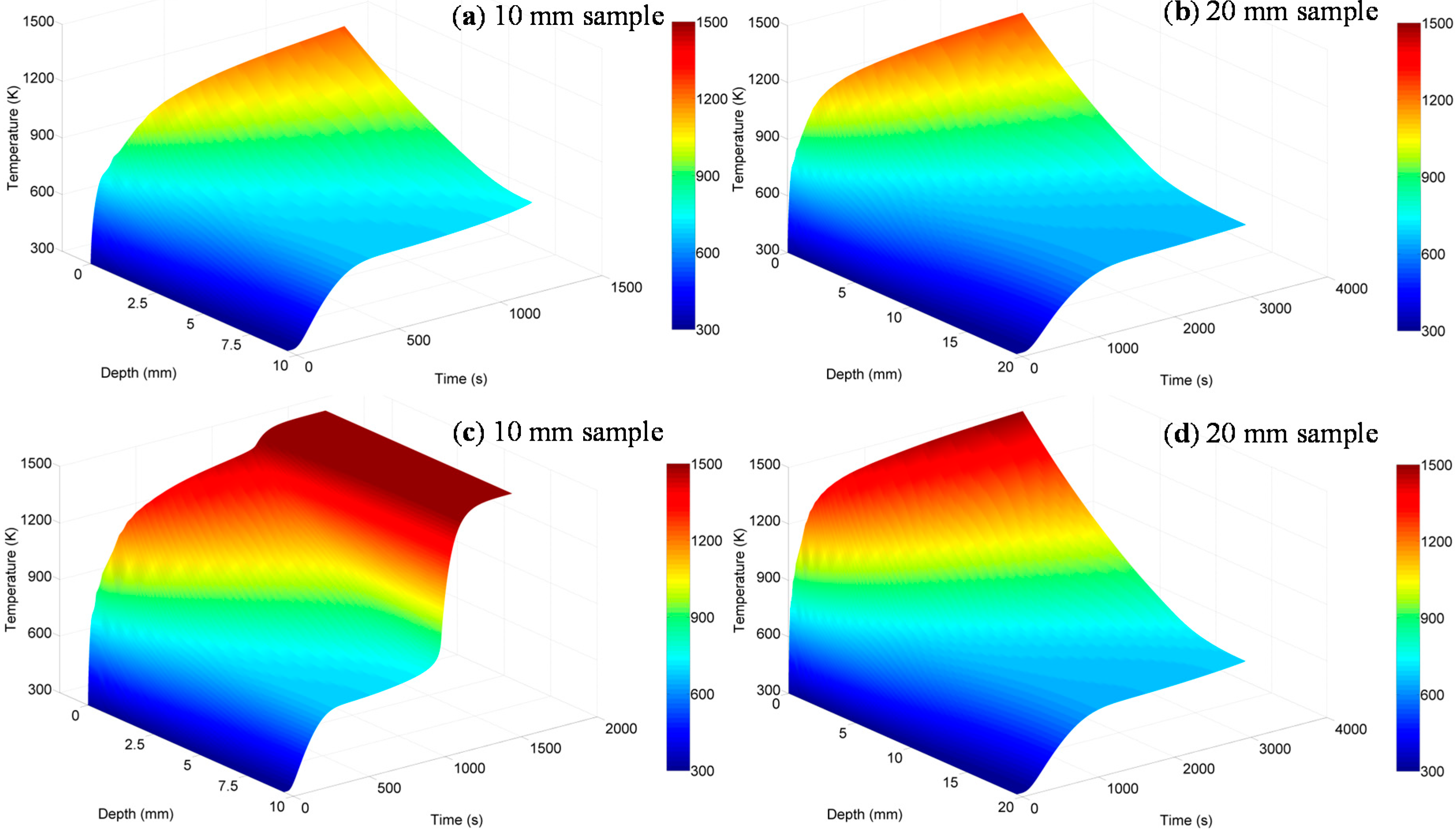
4.1.3. Temperatures Inside the Solid Phase

Figure 3 shows the temperatures inside PMMA slabs under 25, 50 and 75 kW/m2 of heat fluxes, respectively. In these figures, the X-axis represents time, Y-axis shows the depth from the surface and Z-axis depicts the temperature. The color bar on the right hand side of the figure shows a temperature range of 300–800 K.
Figure 3. The temperature profiles inside the PMMA under different heat fluxes: (a,b) 25 kW/m2; (c,d) 50 kW/m2; and (e,f) 75 kW/m2.
Polymers 07 01495 g003
From Figure 3, it can be also seen that the surface temperature increases significantly at the beginning of the runs. Although the increase of the temperature at the bottom of the samples is not so obvious, as compared to the surface temperature, its rate of increase seems to be relatively faster. This could be attributed to the fact that the external heat flux can penetrate the inside of the sample, not only by thermal conduction but also by in-depth radiation. The temperatures inside of the sample slabs decreased, after the burning out of bPMMA, which corresponds with the characteristics expected of materials that leave no char residues after burning. The temperatures inside the PMMA slabs, under 50 and 75 kW/m2 of heat fluxes, were similar to those under 25 kW/m2 heat flux, as shown in Figure 3c–f. It can also be observed that the temperature increases very fast at the beginning and then decrease after burning out of all of the bPMMA.

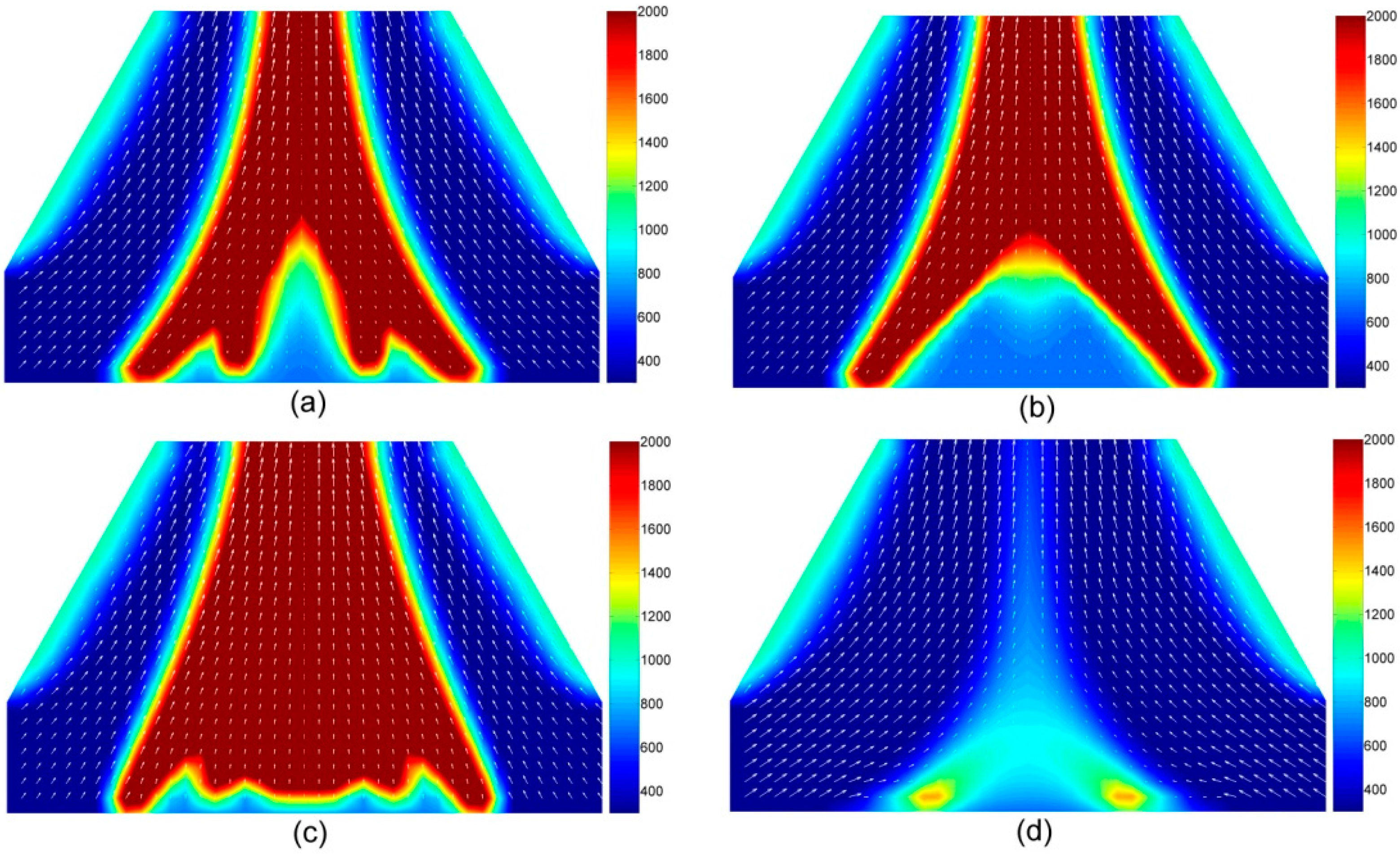
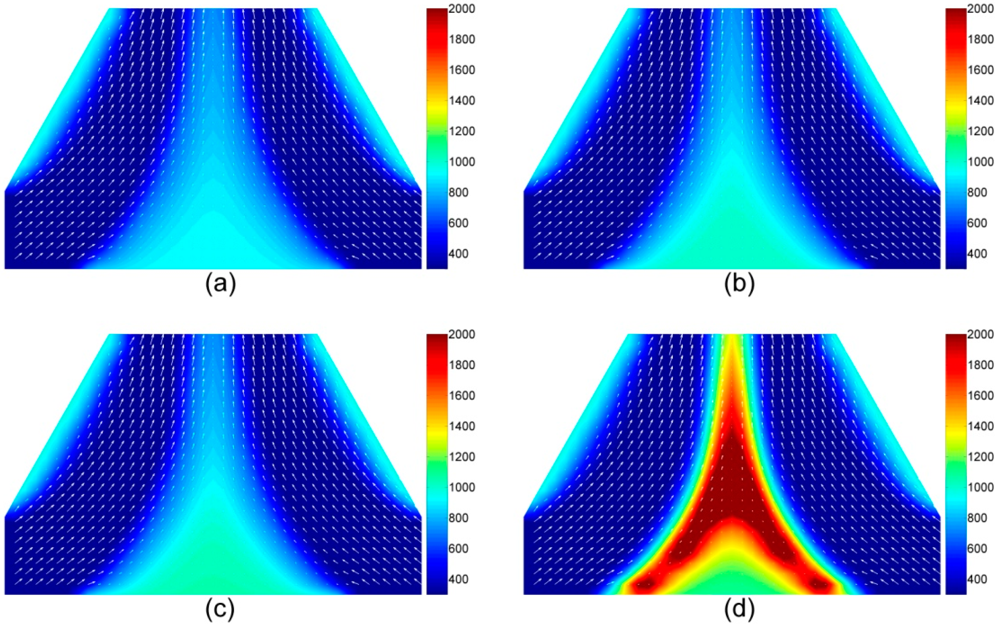
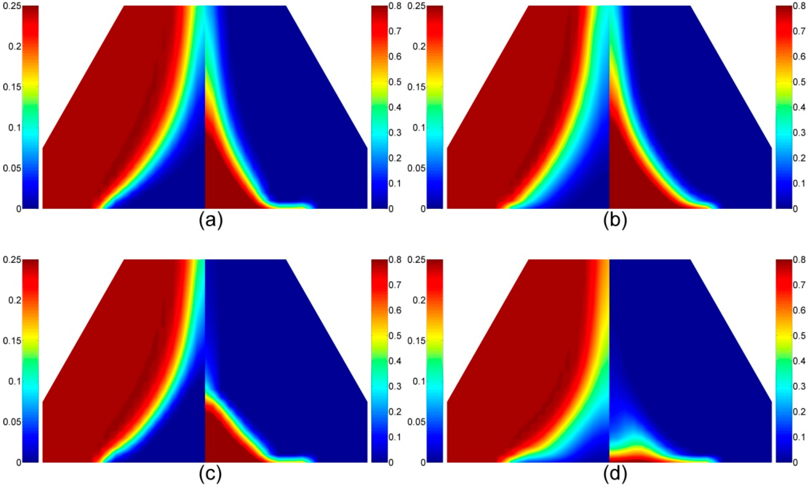
4.1.4. The Temperature and Velocity of Volatiles in the Gas Phase

The temperature and velocity of volatile fragments in the gas phase for PMMA under 75 kW/m2 of heat flux are shown in Figure 4. The color bar on the right hand side of each subset of figures shows a temperature range of 300–2000 K. The selection of peak value of 2000 K in the color bar is to make the temperature range as wide as possible so as to include all the cases with the samples in question, which did not in itself mean that the peak flame temperature is 2000 K. The white arrows in these figures show the gas velocity. Three areas are observed with a higher temperature. The first two areas are near the slope shoulders, which represent the heaters. Temperature of air near the heaters increases because of thermal conduction and convection. The last area is above the bottom of computational domain, which represents sample surface. The volatiles undergo combustion when they are released into the air through the sample surface. As combustion of fuel is an exothermic process, a large amount of heat is released, resulting in high temperature in the surrounding area. In addition, noticeable decreases in temperature can be observed, after the burning out of all the bPMMA, seen in Figure 4d.
Figure 4. Temperature and gas velocity in the gas phase for 10 mm thickness PMMA under 75 kW/m2 heat flux at: (a) 100 s; (b) 200 s; (c) 300 s; and (d) 400 s.
Polymers 07 01495 g004

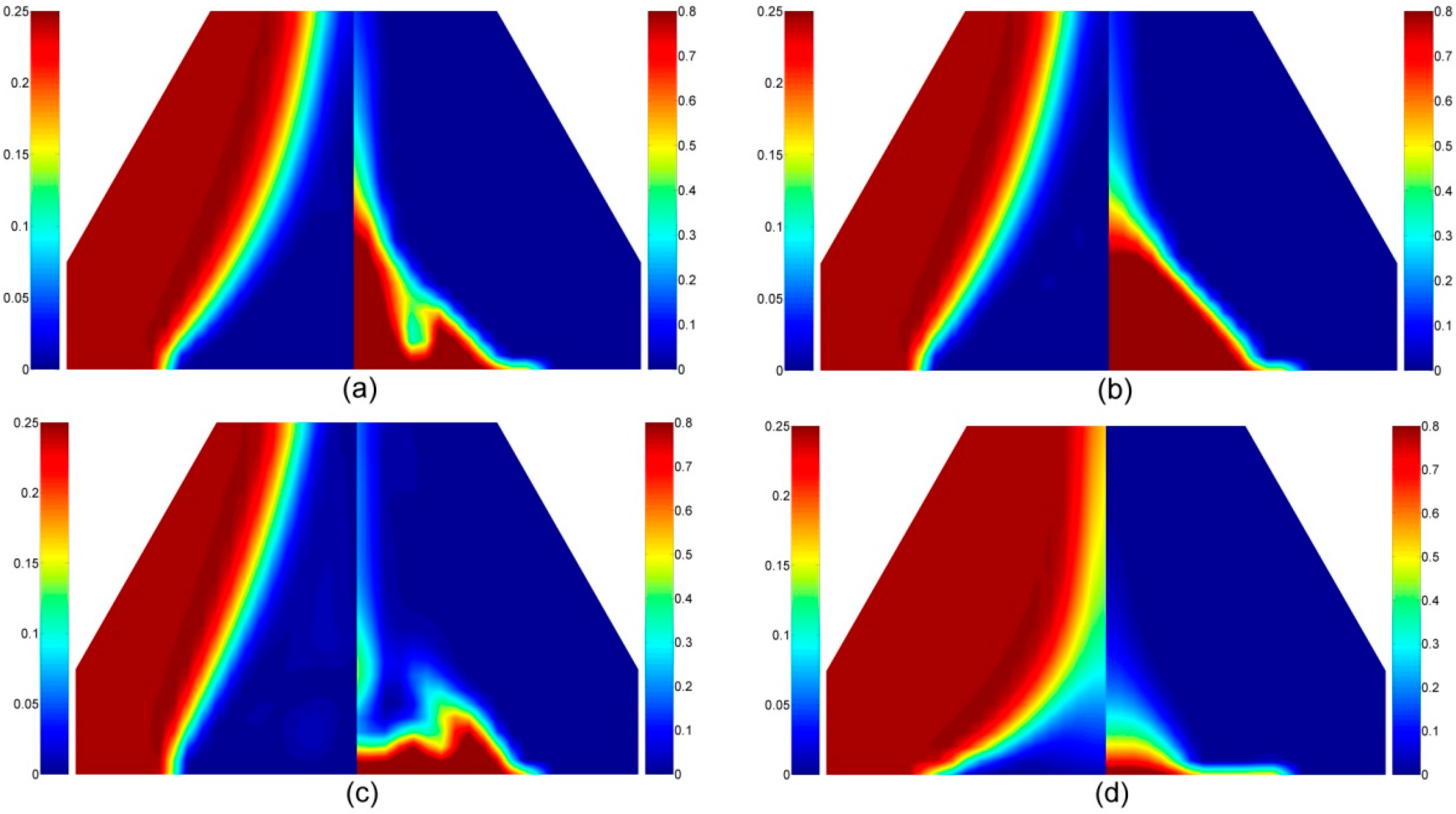
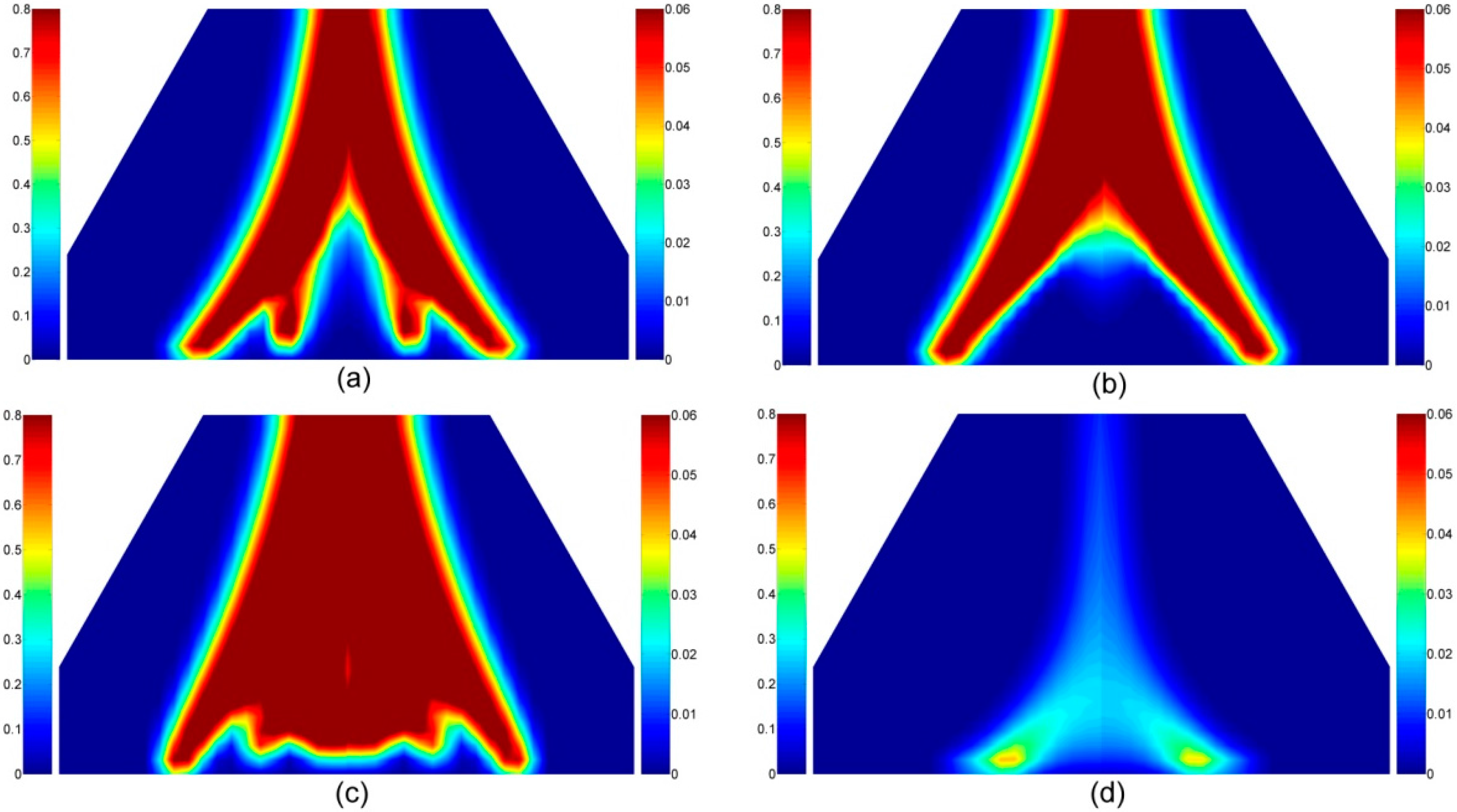
4.1.5. Volatile Components in the Gas Phase

The mass fraction contours of O2 and the fuel for PMMA under 50 kW/m2 of heat flux are shown in Figure 5. For each sub-section in this figure, the left hand side represents the mass fraction contours of O2 and right hand side shows those for the fuel, respectively. The color bars on the left of each sub-section of the figure represent the mass fraction of O2 that ranges from 0 to 0.25, and color bars on the right hand side, with a range of 0–0.8, is those for the fuel. The figures show that mass fraction of O2 in most areas, except in the area above sample surface, are at the ambient value, which is consistent with the structure of computational domain that includes the provision for fresh air to enter from both bottom corners.
Figure 5. Mass fraction of O2 (left half) and Fuel (right half) in the gas phase for 10 mm thickness PMMA under 75 kW/m2 heat flux at: (a) 100 s; (b) 200 s; (c) 300 s; and (d) 400 s.
Polymers 07 01495 g005
The mass fraction contours of CO and CO2 under 75 kW/m2 of heat flux are shown in Figure 6. The high temperature area represents a higher rate of combustion rate of the fuel, thus resulting in a high production of CO and CO2. The mass fractions of CO and CO2 show similar contours as a one-step combustion reaction of fuel was assumed, as given in Equation (15). It is also observed that the mass fraction of CO and CO2 show similar contours with temperature (seen in Figure 4), which indicates that higher amounts of heat cannot be dissipated at lower combustion rates (i.e., lower amounts of CO and CO2).
Figure 6. The mass fractions of CO2 (left hand side) and CO (right hand side) in the gas phase for 10 mm thickness PMMA under 75 kW/m2 heat flux at: (a) 100 s; (b) 200 s; (c) 300 s; and (d) 400 s.
Polymers 07 01495 g006

4.2. Intumescent-Protected Polymer

4.2.1. Thermal Properties of PC

The intumescent protective coating of PC will undergo expansion upon thermal irradiation. The reactions considered for modeling in the present study are listed as follows:
P C       C h a r + F u e l
C h a r       A s h + F u e l
Table 3 shows the thermal properties of PC for the modeling input. As some of the data have not been found to describe pertaining to the transportation of the liquids and gases inside PC slab, they were taken as those based on typical char-formatting sample, like wood. In case of wood sample, a very minor amount of ash is produced from the initially formed char (Equation (21)) [13]. Furthermore, the thermal properties of the char and ash were also assumed to be based on those of wood samples. It should be noted here that some of the assumptions, and the associated parameters taken as the input for modeling, are only very approximate.
Table 3. The thermal properties of PC considered as the input for modeling.
PropertyUnitPCChar/Ash
Pyrolysis reaction rate1/s 2.8 × 10 8 e 1.515 × 10 5 R T [4] 1.31 × 10 8 e 1.34 × 10 5 R T [43]
Densitykg/m31,226.7 (Measured)100 (char); 55 (ash)
Yieldkg/kg0.25 (char yield)0.25 (Ash yield)
Heat of pyrolysiskJ/kg400580
Gas permeabilitym25.80 × 10−175.80 × 10⁻¹⁶
Water permeabilitym23.79 × 10−203.79 × 10⁻¹⁹
Diffusion coefficient of waterm2/s5.11 × 10−95.11 × 10⁻⁸
Diffusion coefficient of gasm2/s1.85 × 10−10;1.85 × 10⁻⁹
Specific heat capacityJ/kg·K1,220 [44]1,350 [45]
Surface emissivity-0.960.90
Thermal conductivityW/m·K0.300.15

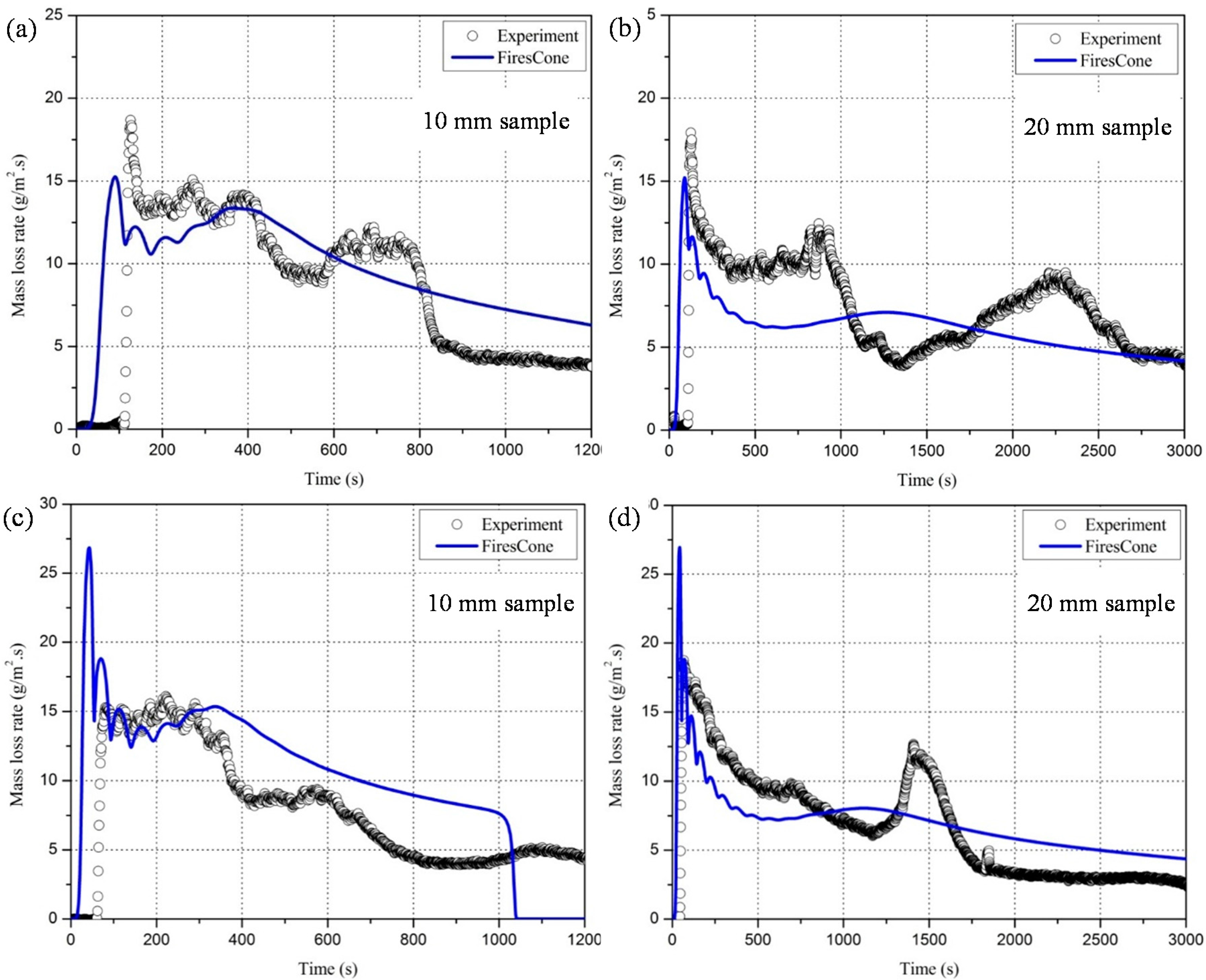
4.2.2. The Mass Loss Rate of the PC Samples

The surface of PC samples, in the form of slabs, underwent expansion soon after start of the irradiance in the cone calorimeter. During the experiment, it was also noticed that the intumescent coating produced expanded char that even touched the cone heater concomitantly, a significant enhancement in the value of the MLR was noted. However, the HRR profiles, primarily measured through the extent of oxygen consumption, were not found to be affected by the above effects. It is known that HRR data generally exhibits a linear relationship with the MLR curve [27,46], which can be expressed by:
M L R = H R R E H C
As the top surface of the degrading samples touched the cone heater, especially towards the latter part of the experimental runs, it was not possible to obtain the complete MLR profiles. The MLR data, for the purpose of comparison, were calculated from the HRR values by using Equation (22). However, such a route was not possible in case of the irradiance level of under 25 kW/m2 as required HRR date could not be obtained as the sample in question did not undergo extensive degradation or combustion. The data for EHC of PC was obtained from reference [27].
Figure 7 shows the comparisons of results obtained through modeling and from experimental runs for PC samples under 50 kW/m2 of heat flux. It can be noticed here that the results from the modeling studies roughly followed the corresponding ones obtained through the experiments. It should be noted here that the additional influence owing to expanding nature of the intumescent protective layer, in real time, complicates the factors influencing the heat and mass transfer though in the system. Furthermore, the irregular nature of the expansion of the intumescent char layers often results in the poor reproducibility of the cone data. Stoliarov et al. [16] observed similar effects when they performed experiments with similar PC samples in a cone calorimeter.
From Figure 7, it can be observed that the peak MLR occurred shortly after the start experimental run, and that the MLR values kept on decreasing thereafter. This could be due to the fact that, upon the production of the initial intumescent char layer, the rates of heat conduction and mass transfer is likely to drop to a significant degree.
Figure 7. The comparison between modeling and experimental curves for PC under heat fluxes of: (a,b) 50 kW/m2; and (c,d) 75 kW/m2.
Polymers 07 01495 g007
Figure 7c,d show the comparison between the modeling and experimental results for PC under 75 kW/m2 of heat flux. It can be seen that for these relatively high heat flux values, the modeling results follow that of the experimental ones more closely. Here again, the peak MLR occurs shortly after start of the experimental run, and suffers a prolonged drop afterwards. A peak near the end of experiment can be observed for 20 mm thickness PC, but it is not obvious for 10 mm thickness PC. This may be because of char pyrolysis or dramatic volume change. Overall, the experimental data seems to be more fluctuant when comparing to the numerical prediction. One of the reasons might be the absence of detailed description about complicated physical processes, such as cracking, irregular expansion, pore formation, etc., in the numerical treatment.

4.2.3. The Temperatures Inside the Solid Phase

The temperatures inside the PC slabs under 50 and 75 kW/m2 heat flux irradiance are shown in Figure 8. The temperature range of the color bar is from 300 to 1500 K.
Figure 8. The temperatures inside PC under heat fluxes for: (a,b) 50 kW/m2; and (c,d) 75 kW/m2.
Polymers 07 01495 g008
In this case, the surface temperature also increases very fast at the beginning, and the rate of increase is also higher for higher irradiance levels. As PC slab becomes translucent, soon after the start of the experiment, the only mode for heat transfer through materials by conduction; this becomes even more difficult after the expansion of the intumescent carbonaceous layer. Therefore, we notice a delay in the increase of the temperature at the bottom surface of the test specimen, and consequently a noticeable temperature gradient across the material.

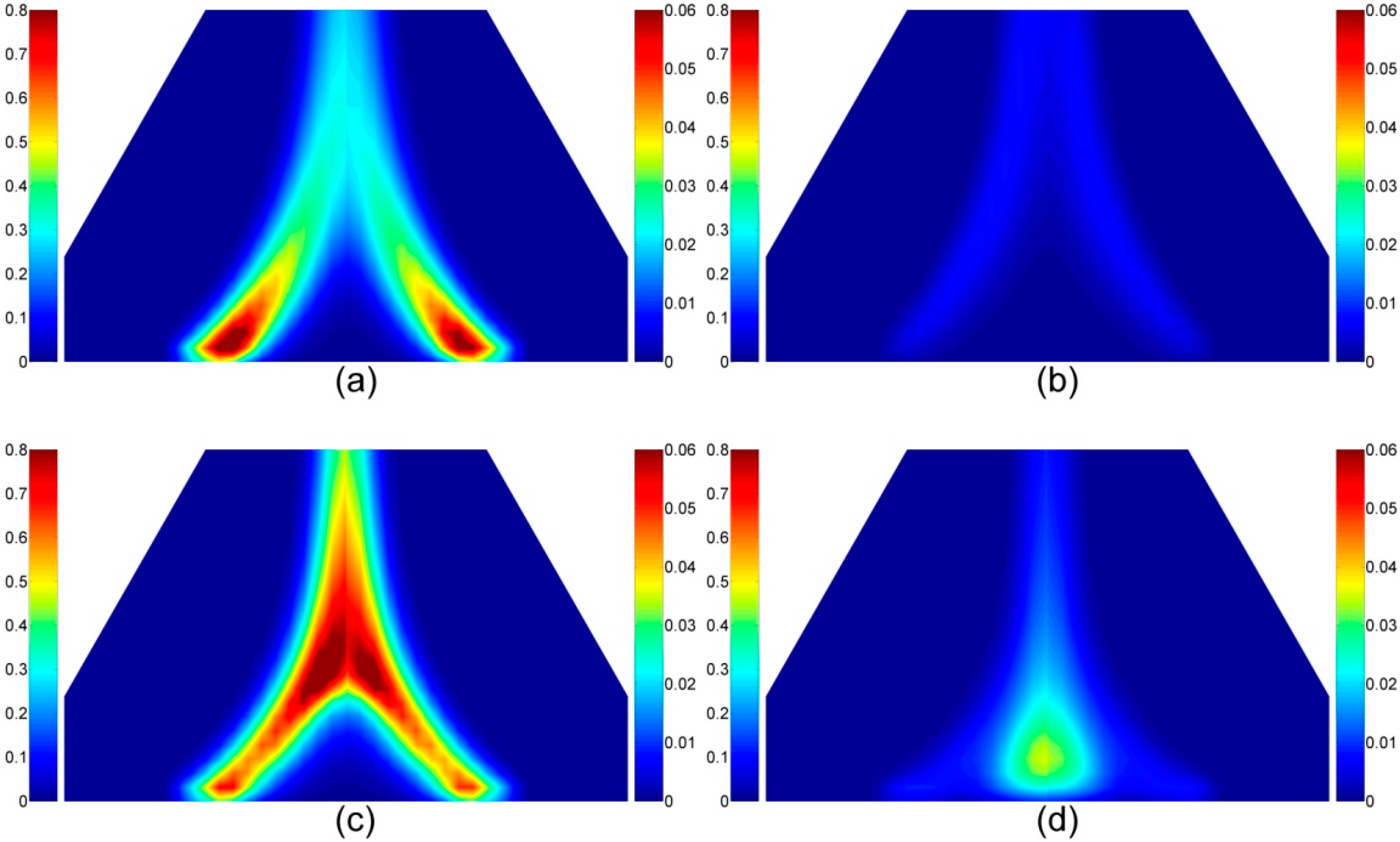
4.2.4. The Temperature and Velocity of the Volatiles in the Gas Phase

Figure 9 shows the temperatures and velocities of the volatile fragments in the gas phase when the PC sample was put under 50 kW/m2 heat flux. Here, the temperature range of the color bar is given from 300 to 2000 K. Figure 9 shows the gas phase temperature when PC slab was put under 50 kW/m2 heat flux. Higher temperature values, especially in Figure 9d, are found to be located at the interface between the fuel and fresh air. This can be attributed to higher rates of the combustion processes happening at the interface, as there is a plenty of fresh air (i.e., oxygen) for the enhanced combustion of the evolved gases from the solid phase.

4.2.5. The Volatiles Species in the Gas Phase

The mass fractions of O2 and fuel for the PC sample under 75 kW/m2 of heat flux are shown in Figure 10. The right hand side of each subset shows the mass fraction of fuel and the left hand side shows the mass fraction of O2. Mass fractions range of the fuel and O2 are in the order of 0–0.8 and 0–0.25, respectively. Similarly, it is shown that mass fraction of O2 in most areas except at the area above the sample surface is at the ambient value. This is expected as the mass fraction of fuel, located above sample surface, increases as the velocity of fuel is enhanced.
Figure 9. The temperatures and velocities of the volatile species in the gas phase for a 10 mm thickness PC under 50 kW/m2 heat flux at: (a) 200 s; (b) 400 s; (c) 600 s; and (d) 1000 s.
Polymers 07 01495 g009
Figure 10. The mass fractions of O2 (left hand side) and fuel (right hand side) in the gas phase for a 10 mm thickness PC under 75 kW/m2 heat flux at: (a) 100 s; (b) 400 s; (c) 800 s; and (d) 1100 s.
Polymers 07 01495 g010
Figure 11 shows the mass fractions of CO and CO2 for a PC sample under 75 kW/m2 of heat flux. The right hand side of each subset depicts the mass fraction of CO, ranging from 0 to 0.06, and the left hand side shows mass fraction contour of CO2, with color bar ranging from 0 to 0.8. As a one-step combustion reaction of fuel was used during numerical modeling, the mass fraction of CO and CO2 show similar contour.
Figure 11. The mass fractions of CO2 (left half) and CO (right half) in the gas phase for 10 mm thick PC under 75 kW/m2 heat flux at: (a) 100 s; (b) 400 s; (c) 800 s; and (d) 1100 s.
Polymers 07 01495 g011

5. Main Conclusions

A mathematical model named “FiresCone” was validated through experimental results from cone calorimetric runs for a non-charring polymer (PMMA) and an intumescent-protected polymer (PC). It was observed that the predictions of mass loss rates obtained through the modeling attempt agreed generally well with those from the experiments for both materials with different thicknesses and under various heat fluxes. It was also observed from both modeling and experimental results that the peak of mass loss rate of the non-charring polymer samples occurred towards the end of experiments, whereas for the intumescent polymer samples, the corresponding change happened at the beginning of the runs. PMMA shows the following differences when compared with charring polymers: the temperature of the bottom surface of PMMA slabs increased at a much faster rate than in the case of the PC samples; temperatures inside PMMA sample decreased after burning out, but the corresponding temperatures for the charring material were maintained at a maximum value towards the end of the each experimental run; the temperatures inside PMMA slab were much lower; and that the heat flux intensity was found to have a limited influence on maximum temperature inside PMMA, than for the PC samples. The differences could be attributed to the prevalence of an in-depth radiative mode of heat transfer, no residue and transparency, respectively. From the validated results obtained through “FiresCone” in the present work, we firmly believe that it is a potential practical tool for investigating the behaviors of fire for a wide variety combustible materials, both charring and non-charring. The future work will be the flame structure simulation and gas volatiles predictions.

Author Contributions

Long Shi performed the experiments, wrote the computer program based on MATLAB and composed the paper. Michael Yit Lin Chew contributed to the analysis of the results, revising computer program, and in the writing and revision of the paper. Vasily Novozhilov contributed to the revision of mathematical model, interpretation of the experimental results and numerical validation, and revision of the paper. Paul Joseph contributed towards the interpretation of the experimental results and revision of the paper.

Conflicts of Interest

The authors declare no conflict of interest.

Nomenclature

Apre-exponential, or frequency factor (s−1)λthermal conductivity (W·m−1·K−1)
Cpspecific heat capacity (J·kg−1·K−1)μdynamic viscosity (Pa·s)
Ddiffusivity coefficient (m2·s−1)υviscosity, stoichiometric coefficient
Eactivation energy (J·mol−1)ρdensity (kg·m−3)
hspecific enthalpy of materials (J)ϕporosity (-)
kreaction rate constant (s−1)
MLRmass loss rate (g·s−1·m−2)Subscripts and Superscripts
norder of reaction (-)extexternal
Nnumber of speciesfflame
Ppressure (Pa)ggas phase, or gas species
q . heat flux (kW·m−2)lliquid water
Qheat of reaction (J·kg−1)pyrpyrolysis process
RUniversal gas constant (J·mol−1·K−1)radradiation process
ttime (s)reacreaction process
Tabsolute temperature (K)ssolid phase, or solid species
u, vvelocity (m·s−1)
x, yCartesian coordinates (m)Abbreviations
Ymass fraction (-)CFDcomputational fluid dynamics
EHCeffective heat of combustion
Greek lettersFuelgeneral designation of gases volatiles
γpermeability (m2)HRRheat release rate
κabsorption coefficient (m−1)MLRmass loss rate
Δchange in variable value (-)PCpolycarbonate
Δhheat of reaction (kJ/kg)PMMApolymethyl methacrylate
Θproduction or reaction rate (kg·m−3·s−1)

References

  1. Stec, A.A.; Hull, T.R.; Purser, D.A.; Purser, J.A. Fire toxicity assessment: comparison of asphyxiant yields from laboratory and large scale flaming fires. In Proceedings of the 11th International Conference on Fire Safety Science, Christchurch, New Zealand, 10–14 February 2014; pp. 404–408.
  2. Li, J.; Stoliarov, S.I. Measurement of kinetics and thermodynamics of the thermal degradation for non-charring polymers. Combust. Flame 2013, 160, 1287–1297. [Google Scholar] [CrossRef]
  3. Griffin, G.J. The modeling of heat transfer across intumescent polymer coatings. J. Fire Sci. 2010, 28, 249–277. [Google Scholar] [CrossRef]
  4. Shi, L.; Chew, M.Y.L. A review of fire processes modeling of combustible materials under external heat flux. Fuel 2013, 106, 30–50. [Google Scholar] [CrossRef]
  5. Karim, M.R.; Naser, J. Progress in numerical modelling of packed bed biomass combustion. In Proceedings of the 19th Australasian Fluid Mechanics Conference, Melbourne, Australia, 8–11 December 2014; pp. 1–4.
  6. Novozhilov, V.; Moghtaderi, B.; Fletcher, D.F.; Kent, J.H. Computational fluid dynamics modelling of wood combustion. Fire Saf. J. 1996, 27, 69–84. [Google Scholar] [CrossRef]
  7. Di Blasi, C. Modeling chemical and physical processes of wood and biomass pyrolysis. Prog. Energy Combust. Sci. 2008, 34, 47–90. [Google Scholar] [CrossRef]
  8. Galgano, A.; di Blasi, C. Modeling the propagation of drying and decomposition fronts in wood. Combust. Flame 2004, 139, 16–27. [Google Scholar] [CrossRef]
  9. Di Blasi, C. Modeling the effects of high radiative heat fluxes on intumescent material decomposition. J. Anal. Appl. Pyrol. 2004, 71, 721–737. [Google Scholar] [CrossRef]
  10. Di Blasi, C. Transition between regimes in the degradation of thermoplastic polymers. Polym. Degrad. Stab. 1999, 64, 359–367. [Google Scholar] [CrossRef]
  11. Kim, E.; Dembsey, N. Parameter estimation for comprehensive pyrolysis modeling: guidance and critical observations. Fire Technol. 2015, 51, 443–477. [Google Scholar] [CrossRef]
  12. Lautenberger, C. Gpyro3D: A three dimensional generalized pyrolysis model. In Proceedings of the 11th International Conference on Fire Safety Science, Christchurch, New Zealand, 10–14 February 2014; pp. 193–207.
  13. Lautenberger, C.; Fernandez-Pello, C. Generalized pyrolysis model for combustible solids. Fire Saf. J. 2009, 44, 819–839. [Google Scholar] [CrossRef]
  14. Stoliarov, S.I.; Leventon, I.T.; Lyon, R.E. Two-dimensional model of burning for pyrolyzable solids. Fire Mater. 2014, 38, 391–408. [Google Scholar] [CrossRef]
  15. Stoliarov, S.I.; Crowley, S.; Lyon, R.E.; Linteris, G.T. Prediction of the burning rates of non-charring polymers. Combust. Flame 2009, 156, 1068–1083. [Google Scholar] [CrossRef]
  16. Stoliarov, S.I.; Crowley, S.; Walters, R.N.; Lyon, R.E. Prediction of the burning rates of charring polymers. Combust. Flame 2010, 157, 2024–2034. [Google Scholar] [CrossRef]
  17. Riccio, A.; Damiano, M.; Zarrelli, M.; Scaramuzzino, F. Three-dimensional modeling of composites fire behavior. J. Reinf. Plast. Compos. 2014, 33, 619–629. [Google Scholar] [CrossRef]
  18. Marquis, D.M.; Pavageau, M.; Guillaume, E.; Chivas-Joly, C. Modelling decomposition and fire behavioubehavior of small samples of a glass-fibre-reinforced polyester/balsa-cored sandwich material. Fire Mater. 2013, 37, 413–439. [Google Scholar] [CrossRef]
  19. Yuen, R.K.K.; Yeoh, G.H.; Davis, G.D.V.; Leonardi, E. Modelling the pyrolysis of wet wood—II. Three-dimensional cone calorimeter simulation. Int. J. Heat Mass Transfer 2007, 50, 4387–4399. [Google Scholar] [CrossRef]
  20. Anderson, C.E.; Wauters, D.K. A thermodynamic heat transfer model for intumescent systems. Int. J. Eng. Sci. 1984, 22, 881–889. [Google Scholar] [CrossRef]
  21. Shi, L.; Chew, M.Y.L. A model to predict carbon monoxide of woods under external heat flux—Part I: Theory. Proced. Eng. 2013, 62, 413–421. [Google Scholar] [CrossRef]
  22. Feih, S.; Mathys, Z.; Gibson, A.G.; Mouritz, A.P. Modelling the compression strength of polymer laminates in fire. Compos. Appl. Sci. Manuf. 2007, 38, 2354–2365. [Google Scholar] [CrossRef]
  23. Henderson, J.B.; Wiecek, T.E. A mathematical model to predict the thermal response of decomposing, expanding polymer composites. J. Compos. Mater. 1987, 21, 373–393. [Google Scholar] [CrossRef]
  24. Staggs, J.E.J. A simple model of polymer pyrolysis including transport of volatiles. Fire Saf. J. 2000, 34, 69–80. [Google Scholar] [CrossRef]
  25. Shi, L.; Chew, M.Y.L.; Novozhilov, V. A model to predict fire behaviors of combustible materials under external heat flux. In Proceedings of the 14th International Conference and Exhibition on Fire and Materials, San Francisco, CA, USA, 2–4 February 2015; pp. 256–270.
  26. Stoliarov, S.I.; Lyon, R.E. Thermo-kinetic model of burning for pyrolyzing materials. In Proceeding of the 9th International Symposium on Fire Safety Science, University of Karlsruhe, German, 21–26 September 2008; pp. 38–50.
  27. Shi, L.; Chew, M.Y.L. Fire behaviors of polymers under autoignition conditions in a cone calorimeter. Fire Saf. J. 2013, 61, 243–253. [Google Scholar] [CrossRef]
  28. Shi, L.; Chew, M.Y.L. Influence of moisture on autoignition of woods in cone calorimeter. J. Fire Sci. 2012, 30, 158–169. [Google Scholar] [CrossRef]
  29. Font, R.; Marcilla, A.; Verdu, E.; Devesa, J. Kinetics of the pyrolysis of almond shells and almond shells impregnated with cobalt dichloride in a fluidized bed reactor and in a pyroprobe 100. Ind. Eng. Chem. Res. 1990, 29, 1846–1855. [Google Scholar] [CrossRef]
  30. Ragland, K.W.; Aerts, D.J. Properties of wood for combustion analysis. Bioresour. Technol. 1991, 37, 161–168. [Google Scholar] [CrossRef]
  31. Di Blasi, C.; Branca, C.; Santoro, A.; Hernandez, E.G. Pyrolytic behavior and products of some wood varieties. Combust. Flame 2001, 124, 165–177. [Google Scholar] [CrossRef]
  32. Thunman, H.; Niklasson, F.; Johnston, F.; Leckner, B. Composition of volatile gases and thermochemical properties of wood for modeling of fixed or fluidized beds. Energy Fuels 2001, 15, 1488–1497. [Google Scholar] [CrossRef]
  33. Di Blasi, C.; Branca, C.; Sparano, S.; Mantia, B.L. Drying characteristics of wood cylinders for conditions pertinent to fixed-bed countercurrent gasification. Biomass Bioenerg. 2003, 25, 45–58. [Google Scholar] [CrossRef]
  34. Bhuiyan, A.A.; Naser, J. Computational modelling of co-firing of biomass with coal under oxy-fuel condition in a small scale furnace. Fuel 2015, 143, 455–466. [Google Scholar] [CrossRef]
  35. Bhuiyan, A.A.; Naser, J. Numerical modelling of oxy fuel combustion, the effect of radiative and convective heat transfer and burnout. Fuel 2015, 139, 268–284. [Google Scholar] [CrossRef]
  36. MatWeb, Your Source for Materials Information. Database of material properties. Available online: www.matweb.com (accessed on 20 April 2015).
  37. Chew, M.Y.L.; Shi, L. Behaviors of materials at elevated temperatures. In Fire Protection—For Building Professionals; NUS Internal Electronic Module Coursework: Singapore, 2012. [Google Scholar]
  38. Schmal, D.; Duyzer, J.H.; van Heuven, J.W. A model for the spontaneous heating of coal. Fuel 1985, 64, 963–972. [Google Scholar] [CrossRef]
  39. Jiang, F.H.; de Ris, J.L.; Khan, M.M. Absorption of thermal energy in PMMA by in-depth radiation. Fire Saf. J. 2009, 44, 106–112. [Google Scholar] [CrossRef]
  40. Gronli, M.G.; Melaaen, M.C. Mathematical model for wood pyrolysis—Comparison of experimental measurements with model predictions. Energy Fuels 2000, 14, 791–800. [Google Scholar] [CrossRef]
  41. Sinha, P.K.; Wang, C.Y. Pore-network modeling of liquid water transport in gas diffusion layer of a polymer electrolyte fuel cell. Electrochimica Acta 2007, 52, 7936–7945. [Google Scholar] [CrossRef]
  42. Tewarson, A. Generation of heat and chemical compounds in fires. In SFPE Handbook of Fire Protection Engineering; National Fire Protection Association: Quincy, MA, USA, 2002. [Google Scholar]
  43. Di Blasi, C. Combustion and gasification rates of lignocellulosic chars. Prog. Energy Combust. Sci. 2009, 35, 121–140. [Google Scholar] [CrossRef]
  44. Lyon, R.E.; Janssens, M.L. Polymer flammability; Report No.: DOT/FAA/AR-05/14; Federal Aviation Administration: Springfield, VA, USA, May 2005.
  45. Alves, S.S.; Figueiredo, J.L. A model for pyrolysis of wet wood. Chem. Eng. Sci. 1989, 44, 2861–2869. [Google Scholar] [CrossRef]
  46. Shi, L.; Chew, M.Y.L. Experimental study of carbon monoxide for woods under spontaneous ignition condition. Fuel 2012, 102, 709–715. [Google Scholar] [CrossRef]

