
Data-Driven Polymer Classification Using BiGRU and Hybrid Metaheuristic Optimization Algorithms


Abstract
1. Introduction
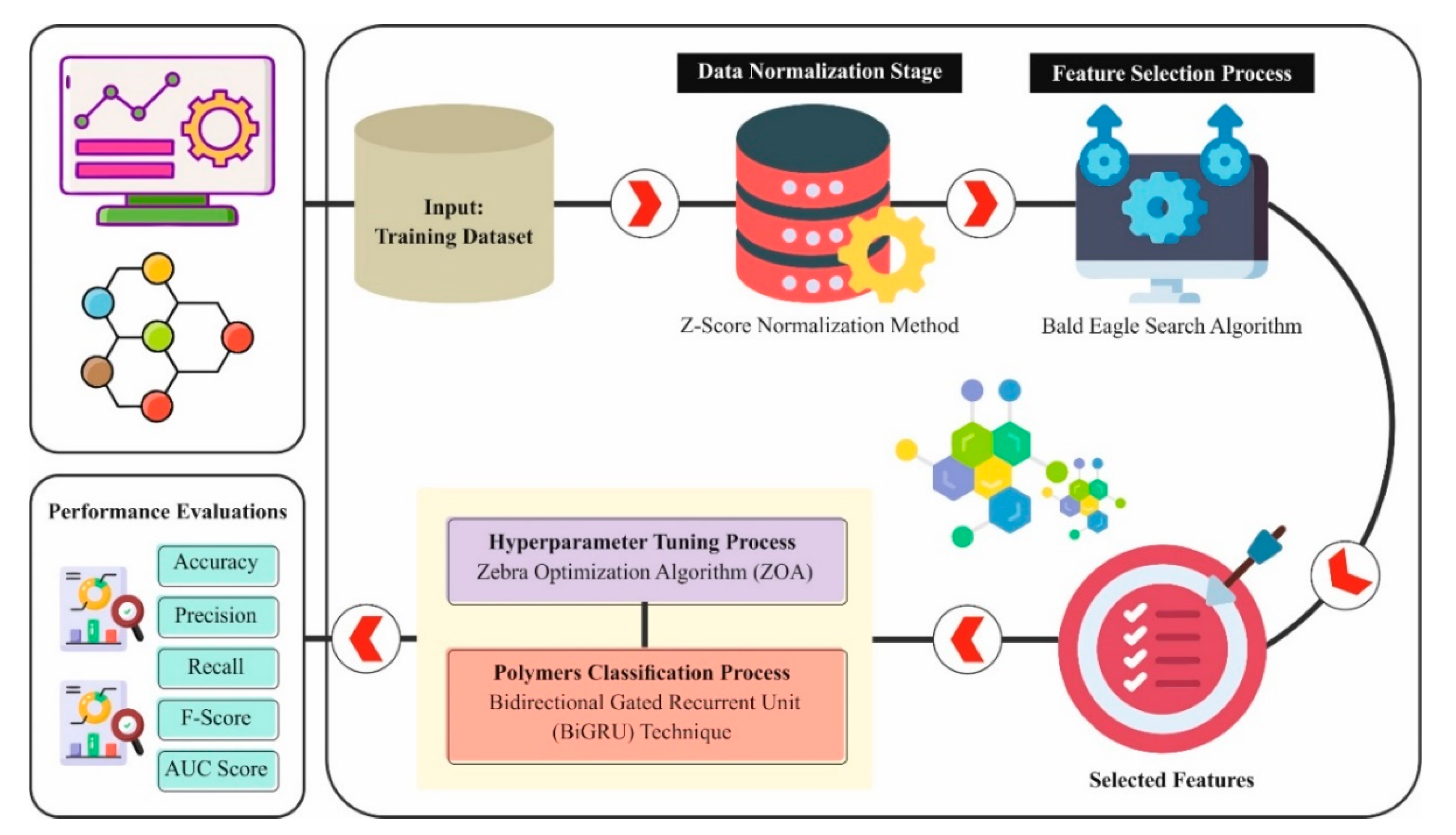
- Z-score normalization to standardize input data distribution;
- Bald Eagle Search (BES) optimization for selecting the most relevant polymer features;
- Bidirectional Gated Recurrent Unit (BiGRU) for learning complex polymer representations;
- Zebra Optimization Algorithm (ZOA) for hyperparameter tuning, optimizing BiGRU performance.
2. Related Works
3. Proposed Methodology
3.1. Pre-Processing
3.2. Feature Selection Process
3.2.1. Initialization
3.2.2. Selecting Phase
3.2.3. Searching Phase
3.2.4. Swooping Phase
3.3. Classification Method
3.4. Hyperparameter Tuning Model
- Learning rate: [0.0001, 0.01];
- Number of GRU units: [32, 256];
- Batch size: [16, 128];
- Dropout rate: [0.1, 0.5];
- Number of epochs: [10, 100]: The optimization objective was to minimize the classification error while balancing the model complexity and training time.
3.4.1. Herding Behavior
3.4.2. Position Updating
3.4.3. Predator Avoidance and Social Interaction
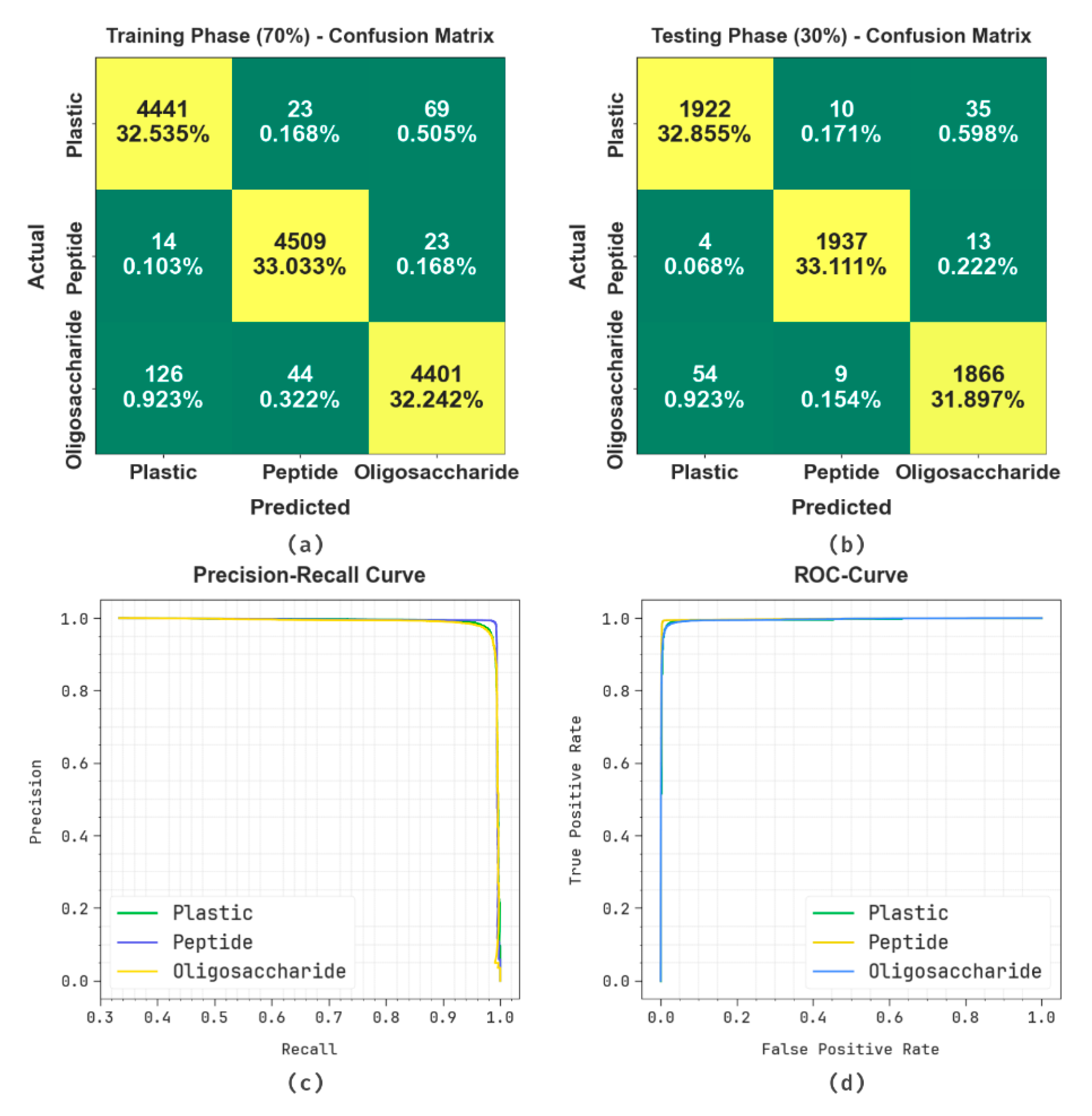
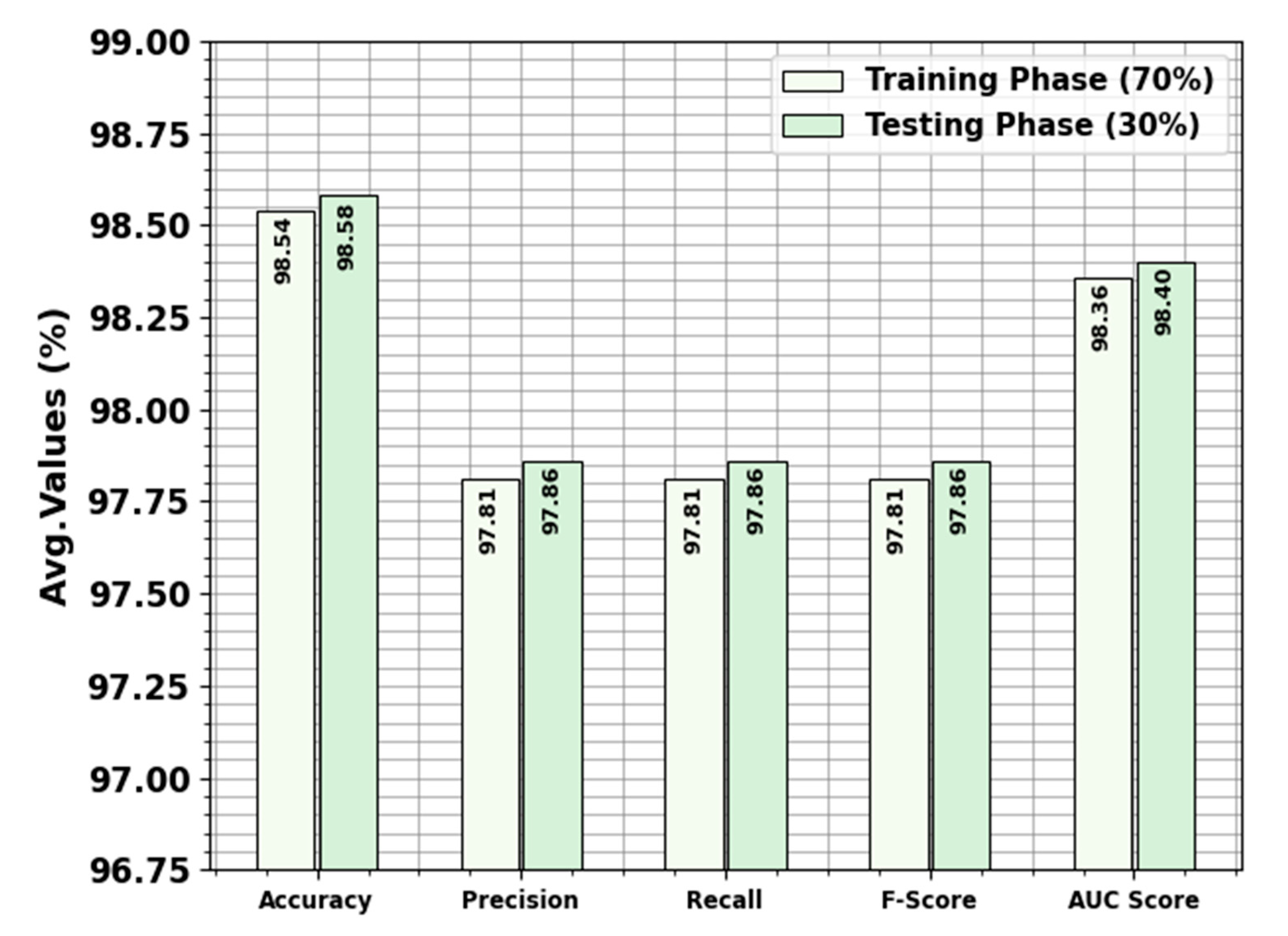
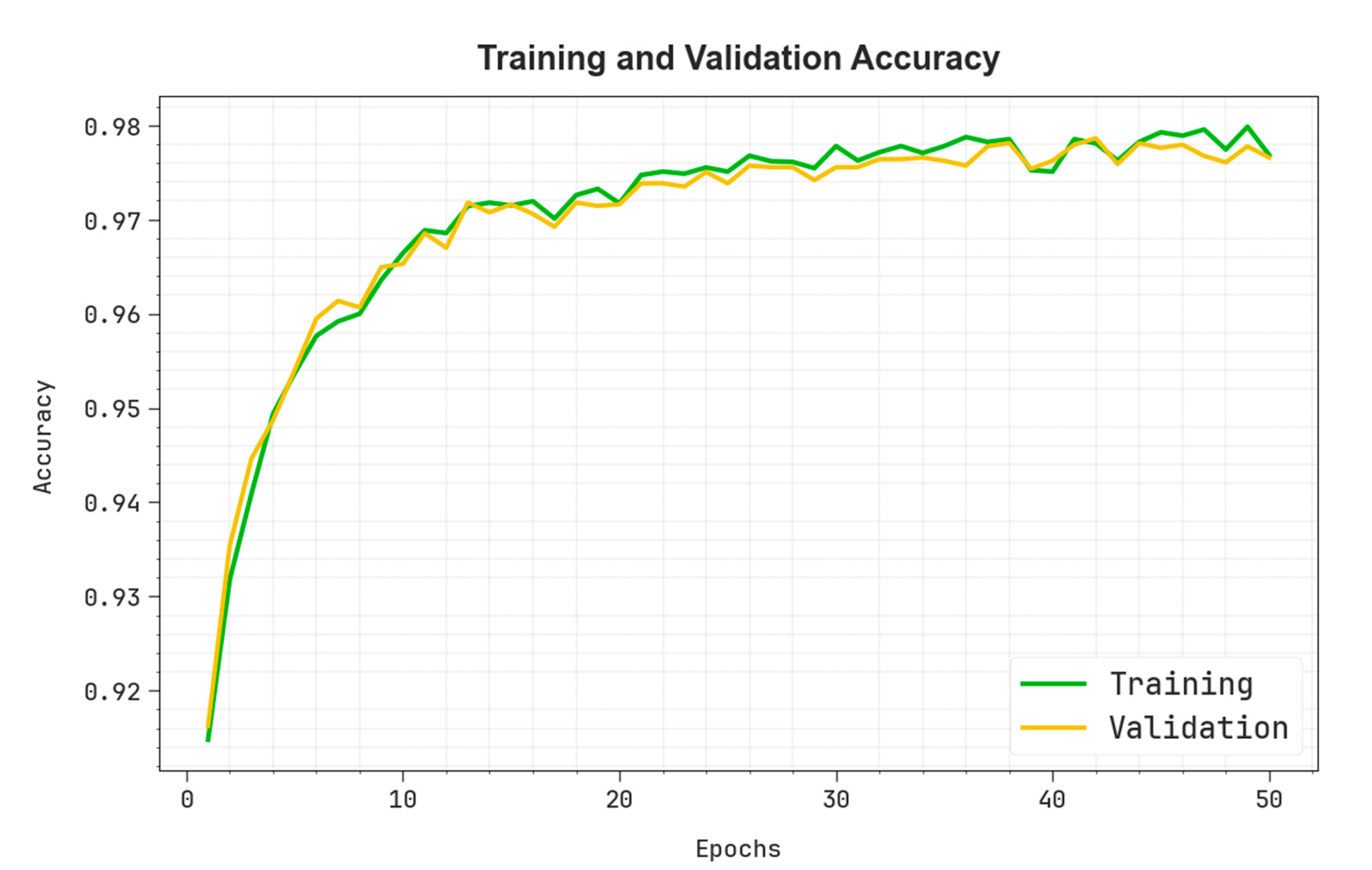
4. Experimental Validation and Results
5. Conclusions
Author Contributions
Funding
Data Availability Statement
Acknowledgments
Conflicts of Interest
References
- Serdeczny, M.P.; Comminal, R.; Pedersen, D.B.; Spangenberg, J. Experimental and analytical study of the polymer melt flow through the hot-end in material extrusion additive manufacturing. Addit. Manuf. 2020, 32, 100997. [Google Scholar] [CrossRef]
- Moslemi, N.; Abdi, B.; Gohery, S.; Sudin, I.; Atashpaz-Gargari, E.; Redzuan, N.; Ayob, A.; Burvill, C.; Su, M.; Arya, F. Thermal response analysis and parameter prediction of additively manufactured polymers. Appl. Therm. Eng. 2022, 212, 118533. [Google Scholar] [CrossRef]
- Dealy, J.M.; Read, D.J.; Larson, R.G. Structure and Rheology of Molten Polymers: From Structure to Flow Behavior and Back Again; Carl Hanser Verlag GmbH Co KG: Munich, Germany, 2018. [Google Scholar]
- Anderegg, D.A.; Bryant, H.A.; Ruffin, D.C.; Skrip, S.M., Jr.; Fallon, J.J.; Gilmer, E.L.; Bortner, M.J. In-situ monitoring of polymer flow temperature and pressure in extrusion based additive manufacturing. Addit. Manuf. 2019, 26, 76–83. [Google Scholar] [CrossRef]
- Wang, S.; Capoen, L.; D’Hooge, D.R.; Cardon, L. Can the melt flow index be used to predict the success of fused deposition modelling of commercial poly (lactic acid) filaments into 3D printed materials? Plast. Rubber Compos. 2018, 47, 9–16. [Google Scholar] [CrossRef]
- Liu, Y.; Yang, C.; Gao, Z.; Yao, Y. Ensemble deep kernel learning with application to quality prediction in industrial polymerization processes. Chemom. Intell. Lab. Syst. 2018, 174, 15–21. [Google Scholar] [CrossRef]
- Gigante, V.; Canesi, I.; Cinelli, P.; Coltelli, M.B.; Lazzeri, A. Rubber toughening of polylactic acid (PLA) with poly (butylene adipate-co-terephthalate)(PBAT): Mechanical properties, fracture mechanics and analysis of ductile-to-brittle behavior while varying temperature and test speed. Eur. Polym. J. 2019, 115, 125–137. [Google Scholar] [CrossRef]
- Volpe, V.; Lanzillo, S.; Affinita, G.; Villacci, B.; Macchiarolo, I.; Pantani, R. Lightweight high-performance polymer composite for automotive applications. Polymers 2019, 11, 326. [Google Scholar] [CrossRef]
- Singh, R.; Kumar, R.; Ahuja, I.P.S. Friction welding for functional prototypes of PA6 and ABS with Al powder reinforcement. Proc. Natl. Acad. Sci. India Sect. A Phys. Sci. 2021, 91, 351–359. [Google Scholar] [CrossRef]
- Yura, H.; Ishihara, M.; Kanatani, Y.; Takase, B.; Hattori, H.; Suzuki, S.; Kawakami, M.; Matsui, T. Interaction study between synthetic glycoconjugate ligands and endocytic receptors using flow cytometry. J. Biochem. 2006, 139, 637–643. [Google Scholar] [CrossRef]
- Velazquez, L.; Palardy, G.; Barbalata, C. A robotic 3D printer for UV-curable thermosets: Dimensionality prediction using a data-driven approach. Int. J. Comput. Integr. Manuf. 2024, 37, 772–789. [Google Scholar] [CrossRef]
- Cui, B.; Wang, H. Compatibility analysis of waste polymer recycling in asphalt binder using molecular descriptor and graph neural network. Resour. Conserv. Recycl. 2025, 212, 107950. [Google Scholar] [CrossRef]
- Shi, J.; Liu, T.; Zhou, L.; Yan, P.; Wang, Z.; Zhang, X. A physics-informed deep learning liquid crystal camera with data-driven diffractive guidance. Commun. Eng. 2024, 3, 46. [Google Scholar] [CrossRef]
- Song, Z.; Feng, Y.; Lu, C. Prediction of the compressive strength and carpet plot for cross-material CFRP laminate based on deep transfer learning. Mater. Sci. Eng. A 2025, 924, 147792. [Google Scholar] [CrossRef]
- Dai, Y.; Wei, J.; Qin, F. Recurrent neural network (RNN) and long short-term memory neural network (LSTM) based data-driven methods for identifying cohesive zone law parameters of nickel-modified carbon nanotube reinforced sintered nano-silver adhesives. Mater. Today Commun. 2024, 39, 108991. [Google Scholar] [CrossRef]
- Ranjbar, I.; Ventikos, Y.; Arashpour, M. Deep learning-based construction and demolition plastic waste classification by resin type using RGB images. Resour. Conserv. Recycl. 2025, 212, 107937. [Google Scholar] [CrossRef]
- Ashok, N.; Soman, K.P.; Samanta, M.; Sruthi, M.S.; Poornachandran, P.; Devi, V.G.S.; Sukumar, N. Polymer and Nanocomposite Informatics: Recent Applications of Artificial Intelligence and Data Repositories. In Advanced Machine Learning with Evolutionary and Metaheuristic Techniques; Springer: Berlin/Heidelberg, Germany, 2024; pp. 297–322. [Google Scholar]
- Si, L.I.U. Multi-modal Deep Learning. Master’s Thesis, Worcester Polytechnic Institute, Worcester, MA, USA, 2022. [Google Scholar]
- Xu, C.; Wang, Y.; Barati Farimani, A. TransPolymer: A Transformer-based language model for polymer property predictions. npj Comput Mater 2023, 9, 64. [Google Scholar] [CrossRef]
- Xu, X.; Wei, Q.; Li, H.; Wang, Y.; Chen, Y.; Jiang, Y. Recognition of polymer configurations by unsupervised learning. Phys. Rev. E 2019, 99, 043307. [Google Scholar] [CrossRef]
- Mehta, M.; Bimrose, M.V.; McGregor, D.J.; King, W.P.; Shao, C. Federated learning enables privacy-preserving and data-efficient dimension prediction and part qualification across additive manufacturing factories. J. Manuf. Syst. 2024, 74, 752–761. [Google Scholar] [CrossRef]
- Ballard, N.; Farajzadehahary, K.; Hamzehlou, S.; Mori, U.; Asua, J.M. Reinforcement learning for the optimization and online control of emulsion polymerization reactors: Particle morphology. Comput. Chem. Eng. 2024, 187, 108739. [Google Scholar] [CrossRef]
- Koinig, G.; Kuhn, N.; Fink, T.; Grath, E.; Tischberger-Aldrian, A. Inline classification of polymer films using Machine learning methods. Waste Manag. 2024, 174, 290–299. [Google Scholar] [CrossRef]
- Zheng, R.; Li, G.; Li, R.; Che, Y.; Wen, H.; Lu, S. A new approach for fire and non-fire aerosols discrimination based on multilayer perceptron trained by modified bonobo optimizer. Clust. Comput. 2025, 28, 167. [Google Scholar] [CrossRef]
- Zhang, L.; Chen, B.; Lyu, D.; Wang, L.; Wang, K. Estimation of Lithium-Ion Battery Health State by Evae and Bigru Based on Eis. SSRN 2025, 5100808. [Google Scholar] [CrossRef]
- Deepanraj, B.; Saravanan, A.M.; Senthilkumar, N.; Afzal, A.A.; Afzal, A.R. Drilling Characteristics Optimization of Polymer Composite Fortified with Eggshells using Box-Behnken Design and Zebra Optimization Algorithm. Results Eng. 2025, 25, 104102. [Google Scholar] [CrossRef]
- Available online: https://www.kaggle.com/code/yeonseokcho/polymers-classification/input (accessed on 2 February 2025).
- Puthukulangara, S.; Govindan, N.P. Deep Learning for Polymer Classification: Automating Categorization of Peptides, Plastics, and Oligosaccharides. J. Adv. Future Res. 2024, 2, 77–86. [Google Scholar]
- Lorenzo-Navarro, J.; Serranti, S.; Bonifazi, G.; Capobianco, G. Performance evaluation of classical classifiers and deep learning approaches for polymers classification based on hyperspectral images. In Advances in Computational Intelligence, Proceedings of the 16th International Work-Conference on Artificial Neural Networks, IWANN 2021, Virtual Event, 16–18 June 2021, Proceedings, Part II 16; Springer International Publishing: Cham, Switzerland, 2021; pp. 281–292. [Google Scholar]


| Class Label | Record Numbers |
|---|---|
| Plastic | 6500 |
| Peptide | 6500 |
| Oligosaccharide | 6500 |
| Total Records | 19,500 |
| S.no | Smiles | Label |
|---|---|---|
| 1 | “C(Cl)CCC(c1ccccc1)CCC(Cl)C” | Plastic |
| 2 | “CC(c1ccccc1)CCC(CC)CCCC(C)C” | Plastic |
| 3 | “OC(=O)[C@]([H])(CCSC)NC(=O)[C@]([H])(CC(C)C)NC(=O)[C@]([H])(CC(C)C)N” | Peptide |
| 4 | “OC(=O)[C@]([H])(CO)NC(=O)[C@]([H])(C1CCCN1)NC(=O)[C@]([H])([H])N” | Peptide |
| 5 | “O[C@]([C@]([H])(CO)O[C@](O)([H])[C@]([H])1O)([H])[C@]1([H])O[C@]([C@]([H])(CO)O[C@](O)([H])[C@]([H])1O)([H])[C@]1([H])O[C@@]([C@]([H])(CO)O[C@](O)([H])[C@@]([H])1O)([H])[C@]1([H])O” | Oligosaccharide |
| 6 | “O[C@]([C@@]([H])(CO)O[C@@](O)([H])[C@]([H])1O)([H])[C@@]1([H])N[C@]([C@]([H])(CO)O[C@](O)([H])[C@]([H])1O)([H])[C@]1([H])O[C@]([C@]([H])(CO)O[C@](O)([H])[C@]([H])1O)([H])[C@@]1([H])O[C@]([C@]([H])(CO)O[C@](O)([H])[C@]([H])1O)([H])[C@@]1([H])O” | Oligosaccharide |
| Class Labels | |||||
|---|---|---|---|---|---|
| TRAPS (70%) | |||||
| Plastic | 98.30 | 96.94 | 97.97 | 97.45 | 98.22 |
| Peptide | 99.24 | 98.54 | 99.19 | 98.86 | 99.23 |
| Oligosaccharide | 98.08 | 97.95 | 96.28 | 97.11 | 97.63 |
| Average | 98.54 | 97.81 | 97.81 | 97.81 | 98.36 |
| TESPS (30%) | |||||
| Plastic | 98.24 | 97.07 | 97.71 | 97.39 | 98.11 |
| Peptide | 99.38 | 99.03 | 99.13 | 99.08 | 99.32 |
| Oligosaccharide | 98.10 | 97.49 | 96.73 | 97.11 | 97.75 |
| Average | 98.58 | 97.86 | 97.86 | 97.86 | 98.40 |
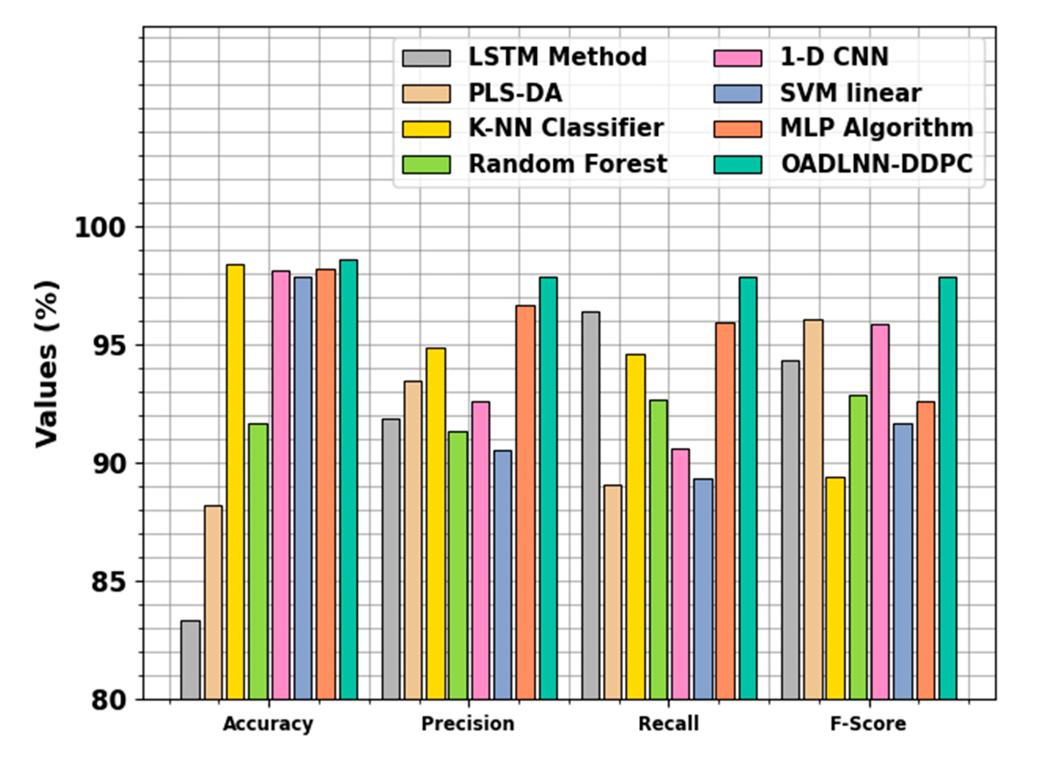
| Technique | ||||
|---|---|---|---|---|
| LSTM Method | 83.37 | 91.89 | 96.42 | 94.33 |
| PLS-DA | 88.18 | 93.49 | 89.06 | 96.08 |
| K-NN Classifier | 98.36 | 94.86 | 94.60 | 89.41 |
| Random Forest | 91.68 | 91.35 | 92.66 | 92.84 |
| 1-D CNN | 98.10 | 92.58 | 90.59 | 95.84 |
| SVM linear | 97.86 | 90.56 | 89.36 | 91.64 |
| MLP Algorithm | 98.19 | 96.65 | 95.91 | 92.57 |
| OADLNN-DDPC | 98.58 | 97.86 | 97.86 | 97.86 |
| Technique | ET (min) |
|---|---|
| LSTM Method | 39 |
| PLS-DA | 34 |
| K-NN Classifier | 23 |
| Random Forest | 36 |
| 1-D CNN | 39 |
| SVM linear | 38 |
| MLP Algorithm | 48 |
| OADLNN-DDPC | 10 |
Disclaimer/Publisher’s Note: The statements, opinions and data contained in all publications are solely those of the individual author(s) and contributor(s) and not of MDPI and/or the editor(s). MDPI and/or the editor(s) disclaim responsibility for any injury to people or property resulting from any ideas, methods, instructions or products referred to in the content. |
© 2025 by the authors. Licensee MDPI, Basel, Switzerland. This article is an open access article distributed under the terms and conditions of the Creative Commons Attribution (CC BY) license (https://creativecommons.org/licenses/by/4.0/).
Share and Cite
Parvez, M.A.; Mehedi, I.M. Data-Driven Polymer Classification Using BiGRU and Hybrid Metaheuristic Optimization Algorithms. Polymers 2025, 17, 1894. https://doi.org/10.3390/polym17141894
Parvez MA, Mehedi IM. Data-Driven Polymer Classification Using BiGRU and Hybrid Metaheuristic Optimization Algorithms. Polymers. 2025; 17(14):1894. https://doi.org/10.3390/polym17141894
Chicago/Turabian StyleParvez, Mohammad Anwar, and Ibrahim M. Mehedi. 2025. "Data-Driven Polymer Classification Using BiGRU and Hybrid Metaheuristic Optimization Algorithms" Polymers 17, no. 14: 1894. https://doi.org/10.3390/polym17141894
APA StyleParvez, M. A., & Mehedi, I. M. (2025). Data-Driven Polymer Classification Using BiGRU and Hybrid Metaheuristic Optimization Algorithms. Polymers, 17(14), 1894. https://doi.org/10.3390/polym17141894