

Deformation Behavior Investigation of Auxetic Structure Made of Poly(butylene adipate-co-terephthalate) Biopolymers Using Finite Element Method
 , ,
, ,  ,
,
Abstract
:1. Introduction
2. Materials and Experiments
2.1. Materials
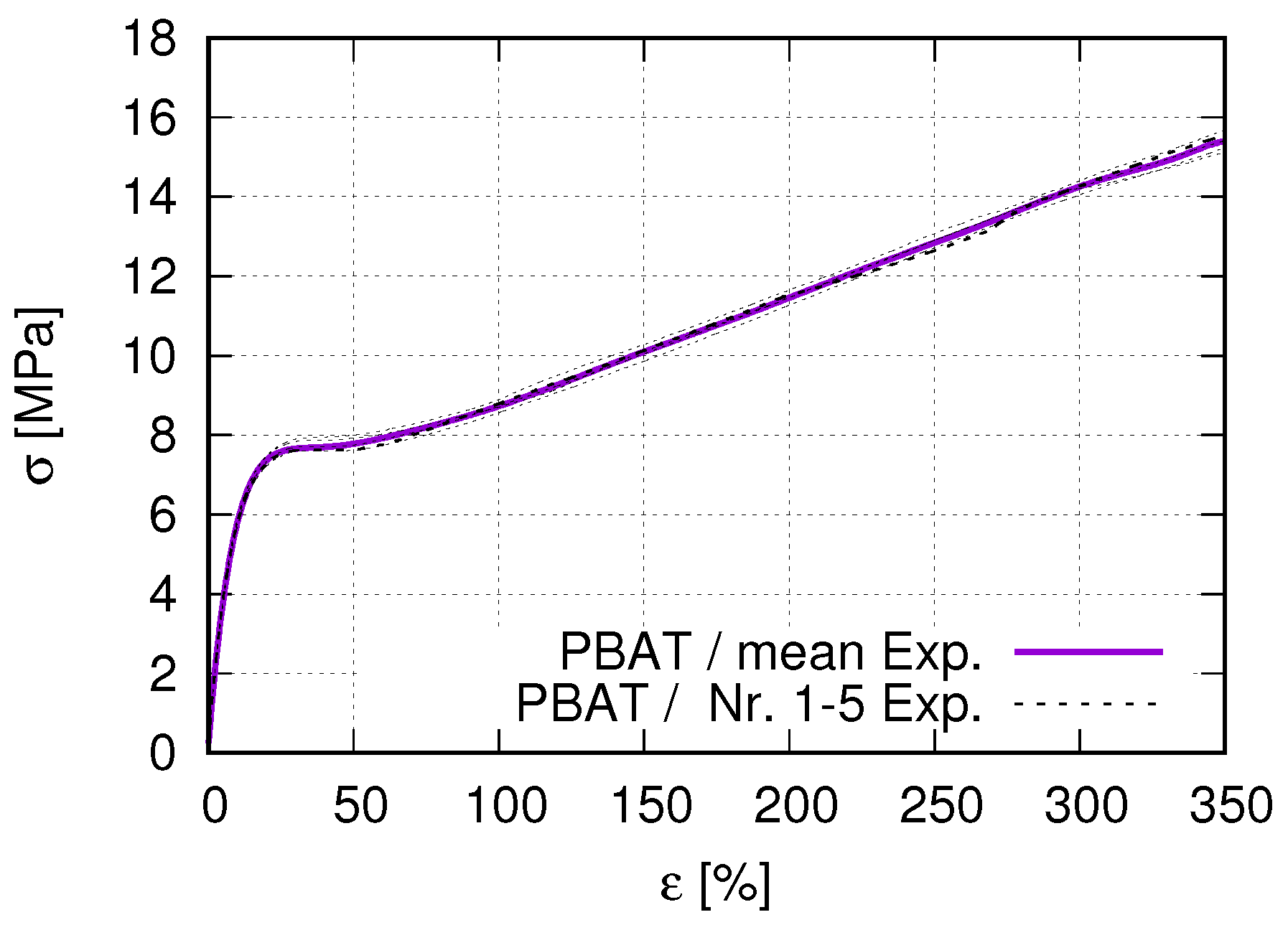
2.2. Tensile Test
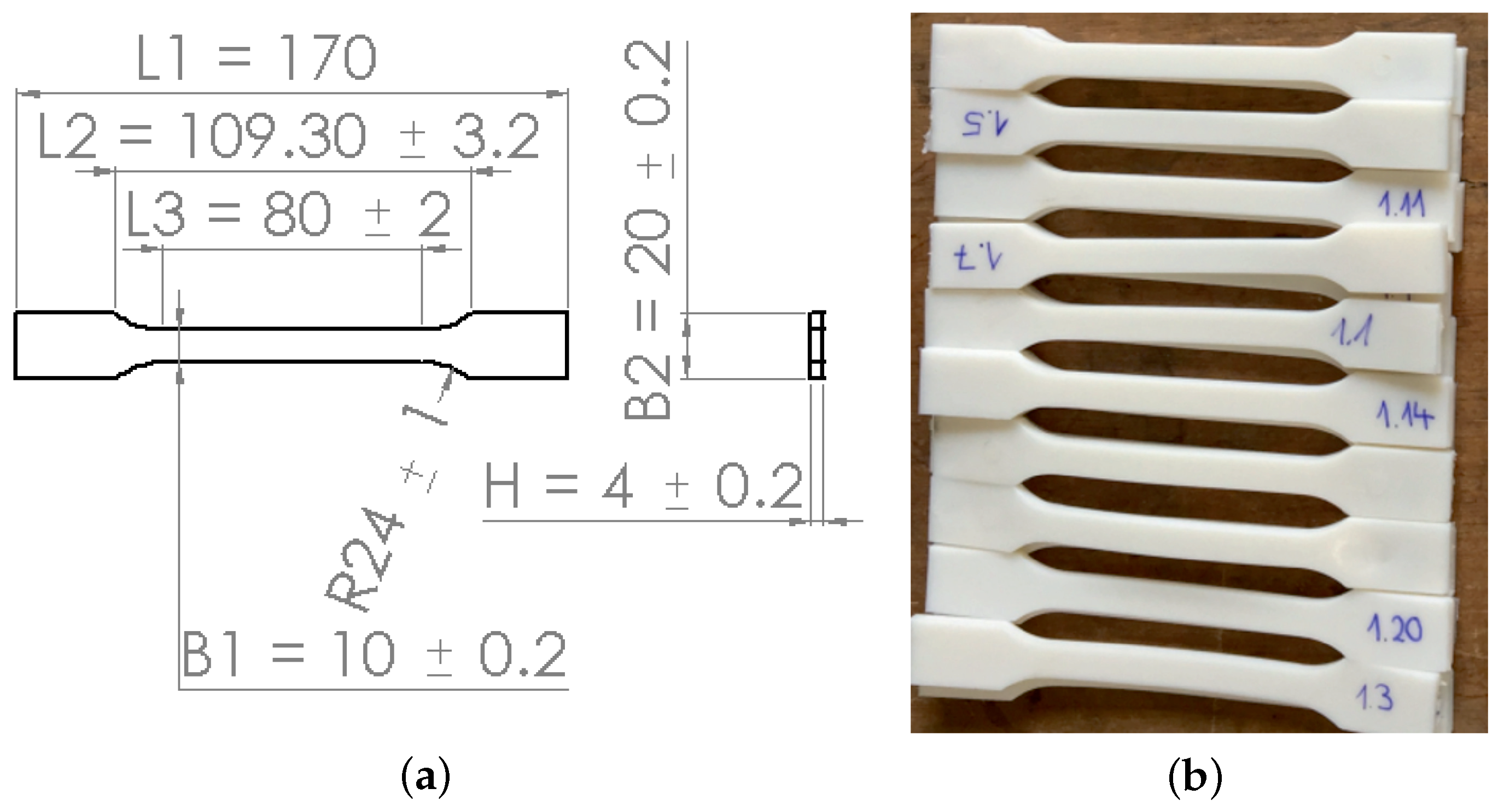
2.2.1. Standard Tensile Test Specimen
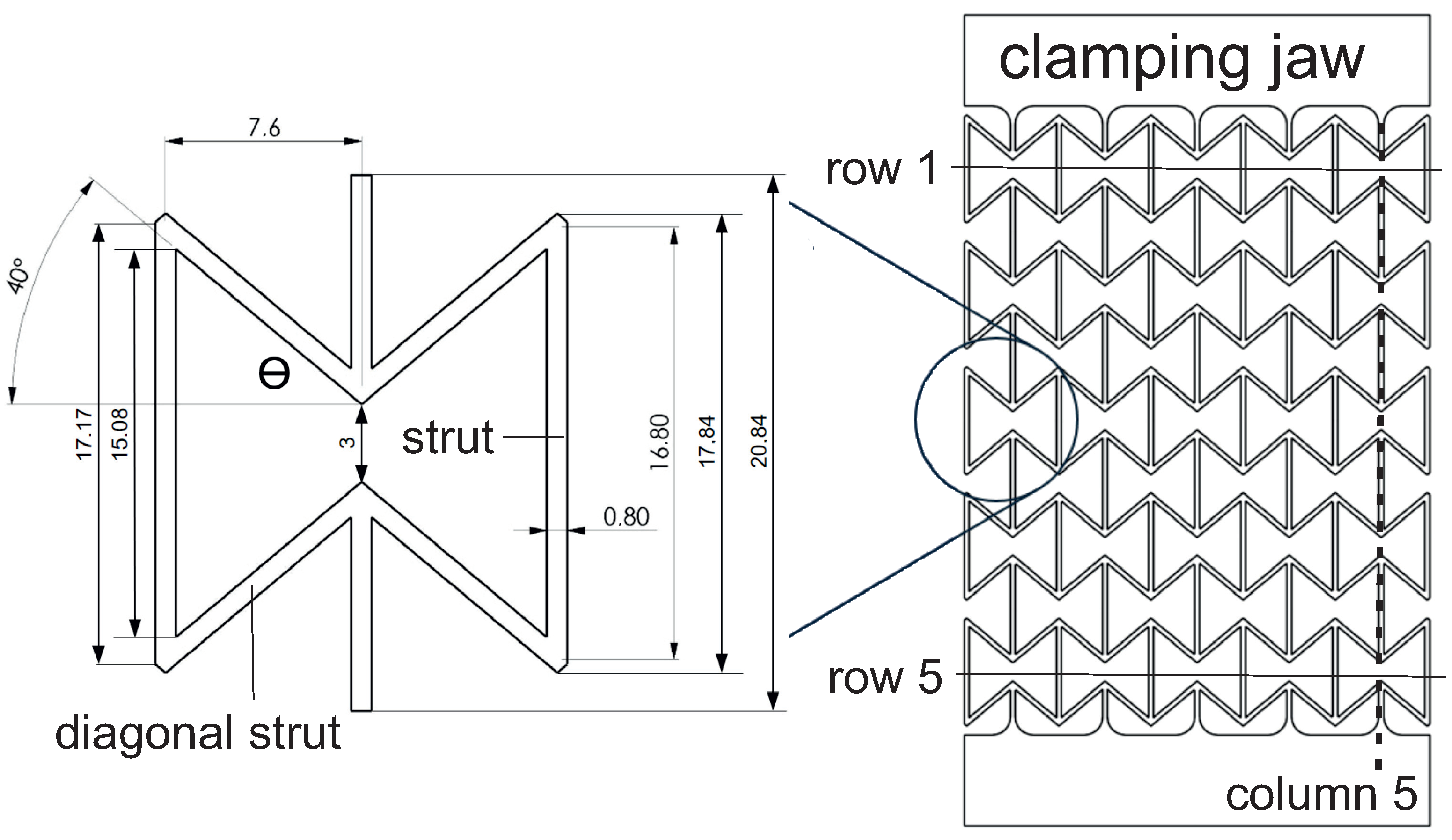
2.2.2. Auxetic Tensile Test Specimen
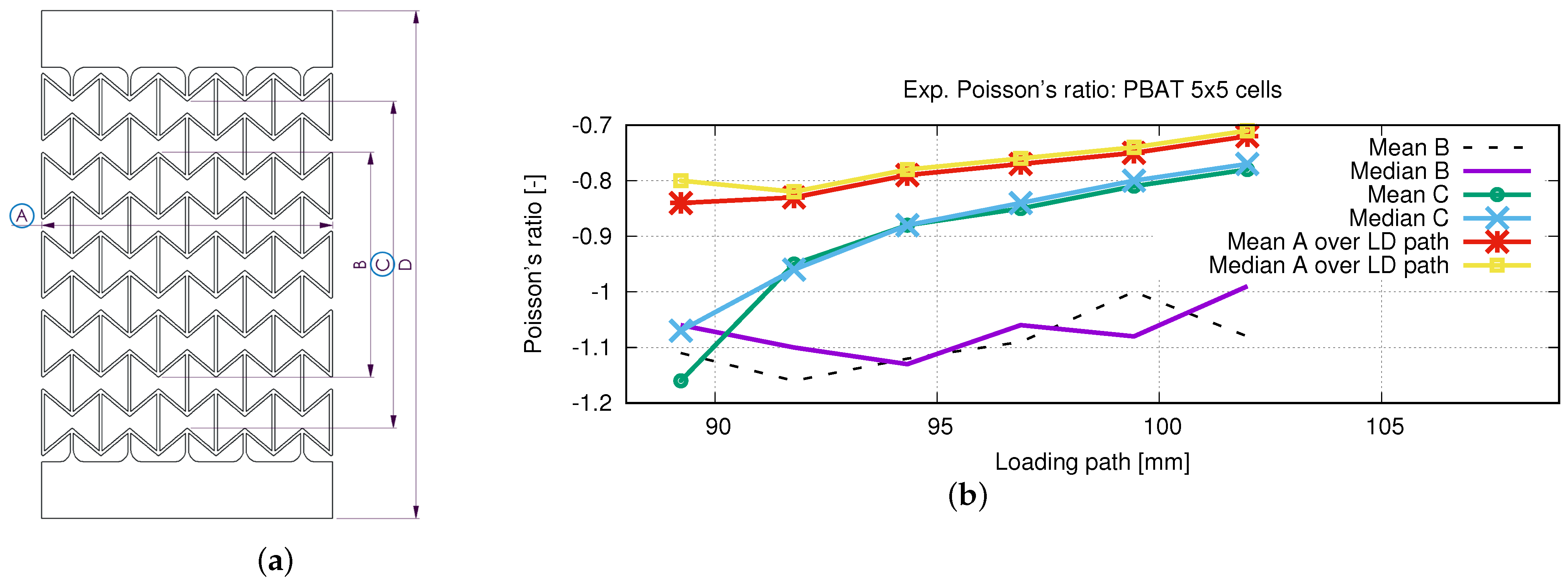
2.2.3. Poisson’s Ratio Calculation from Measured Data
3. FE Simulation
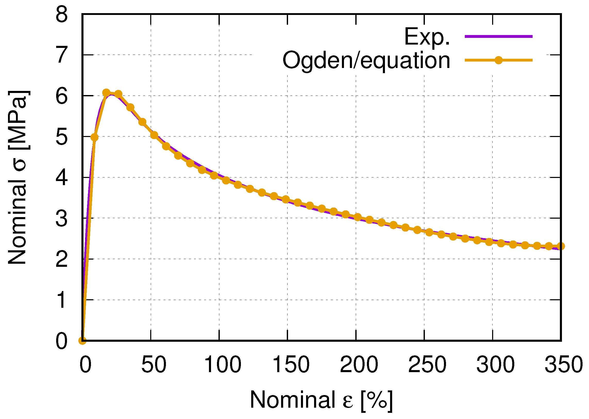
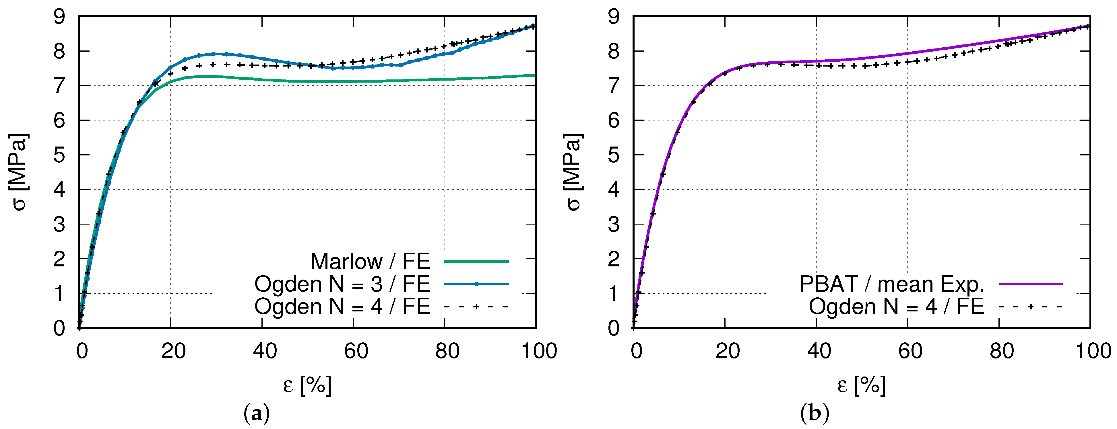
3.1. Material Model
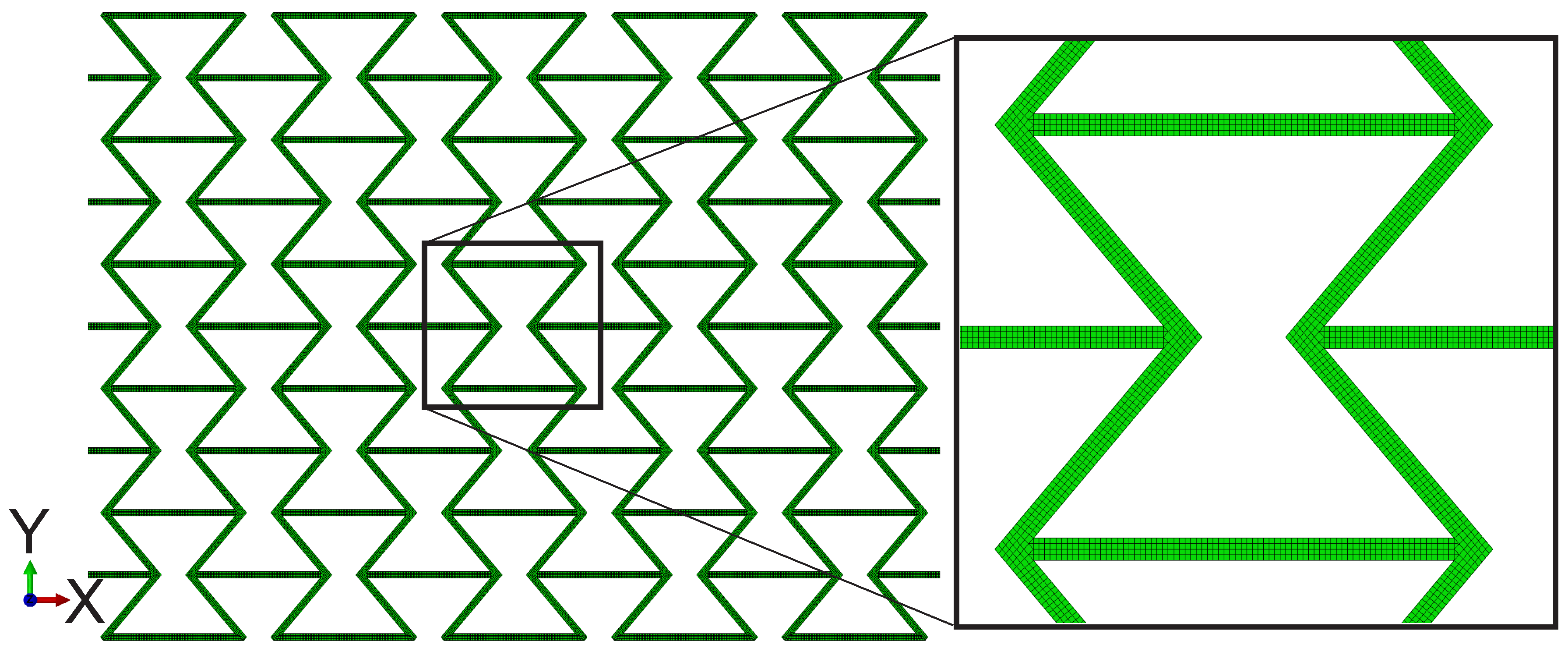
3.2. Applied Structure and Boundary Conditions
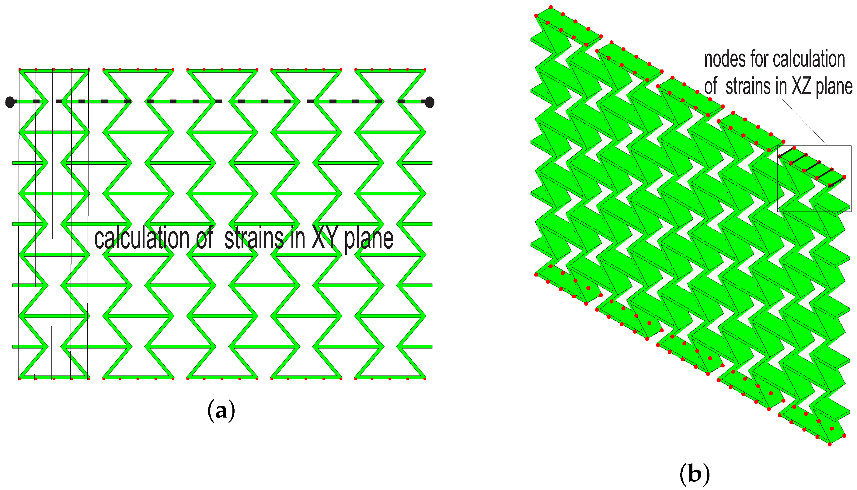
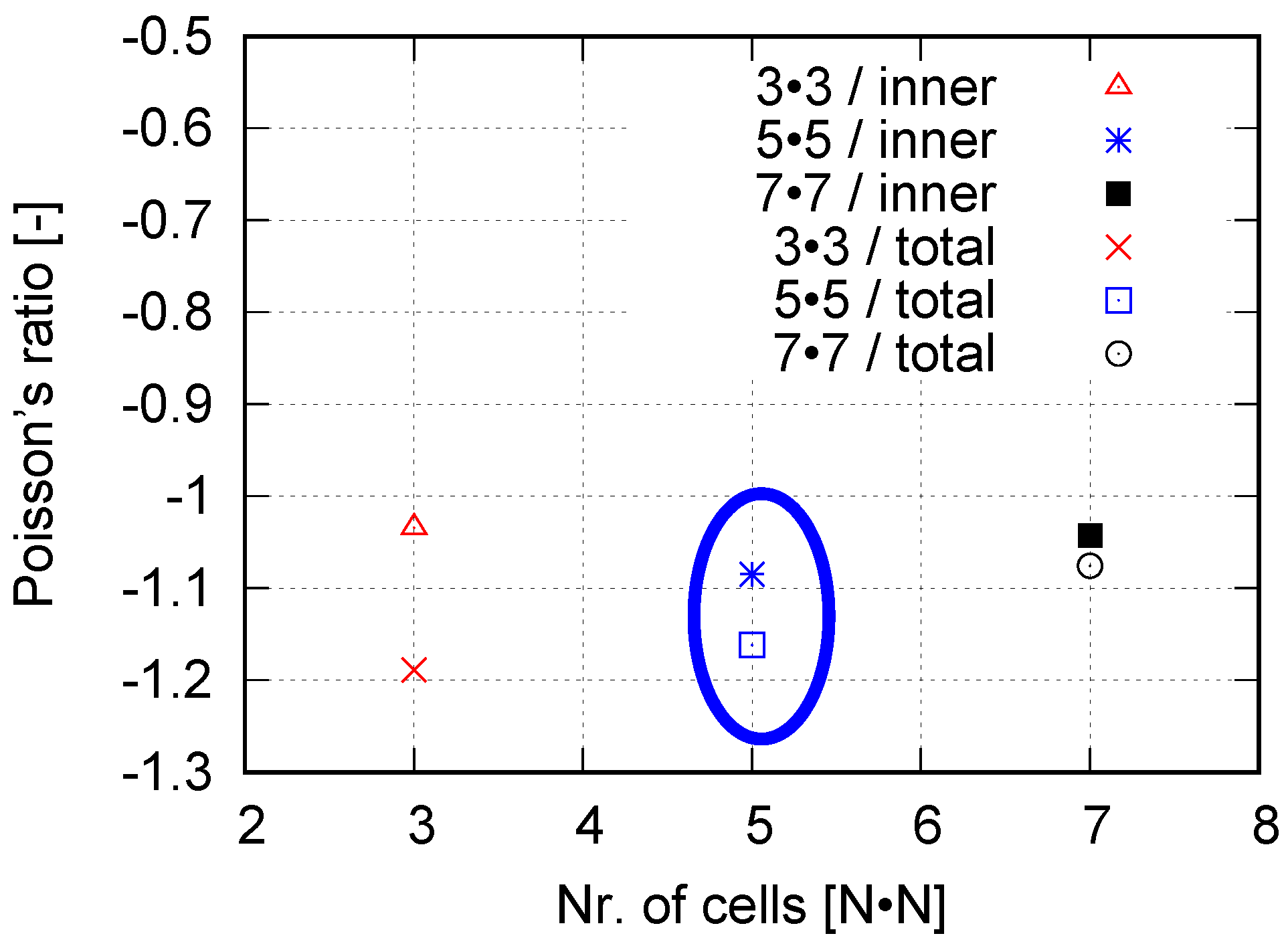
3.3. Poisson’s Ratio Calculation from FE Results
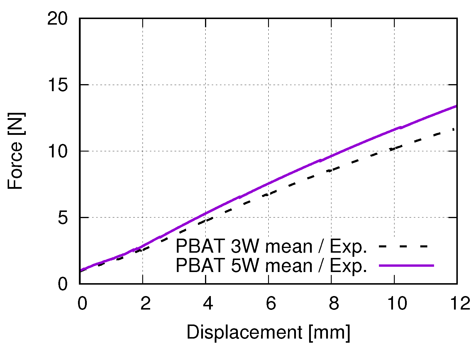
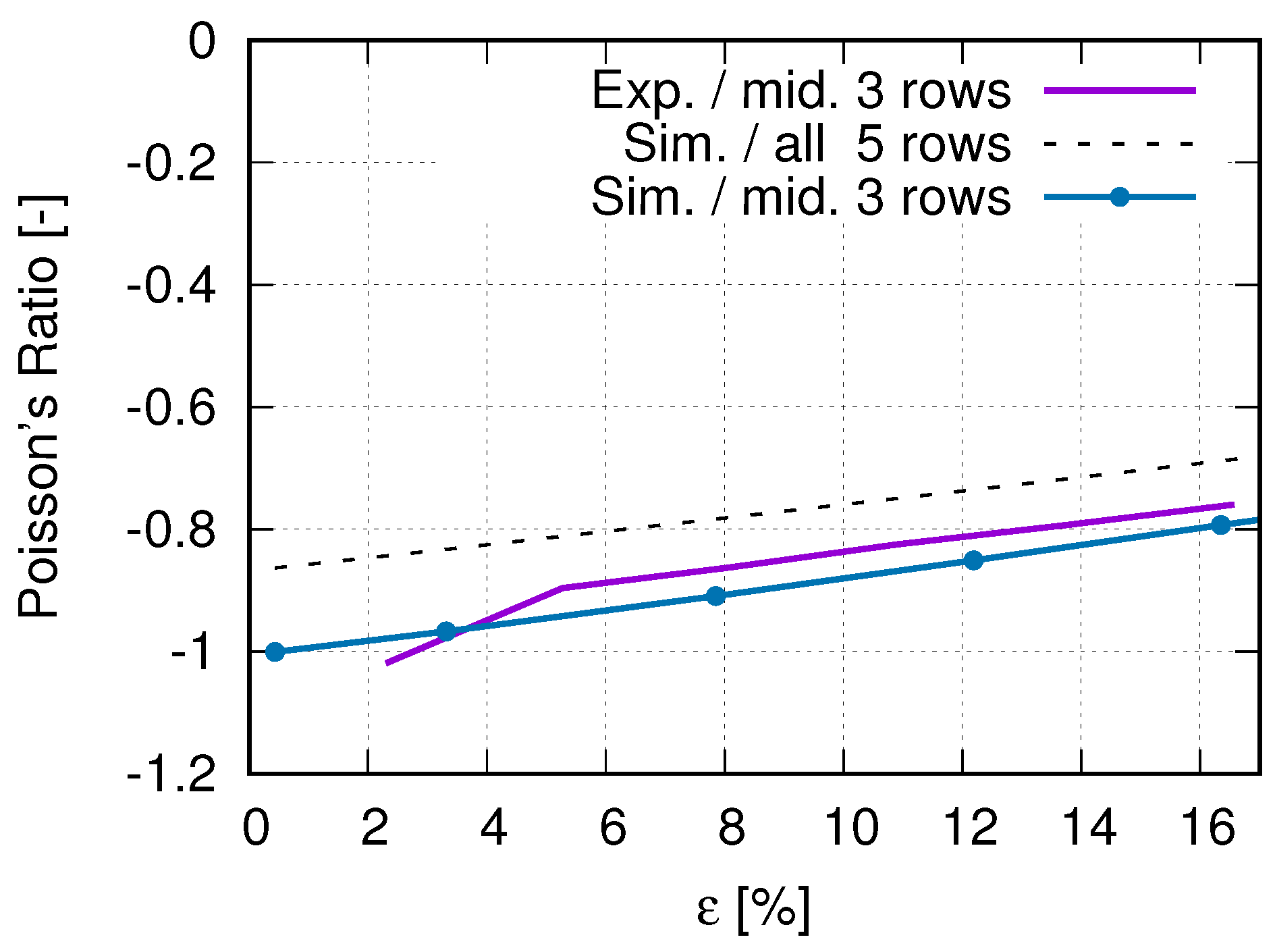
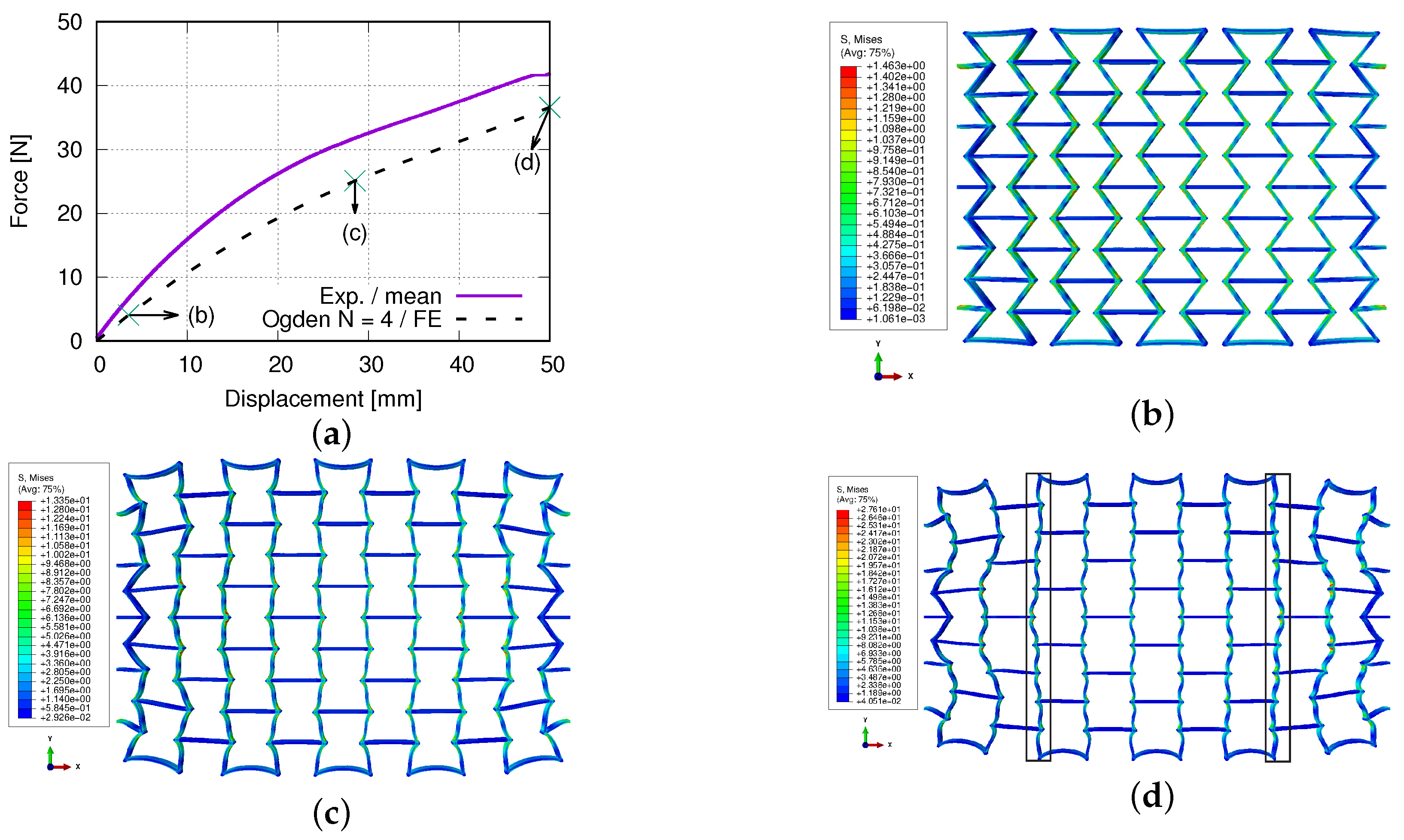
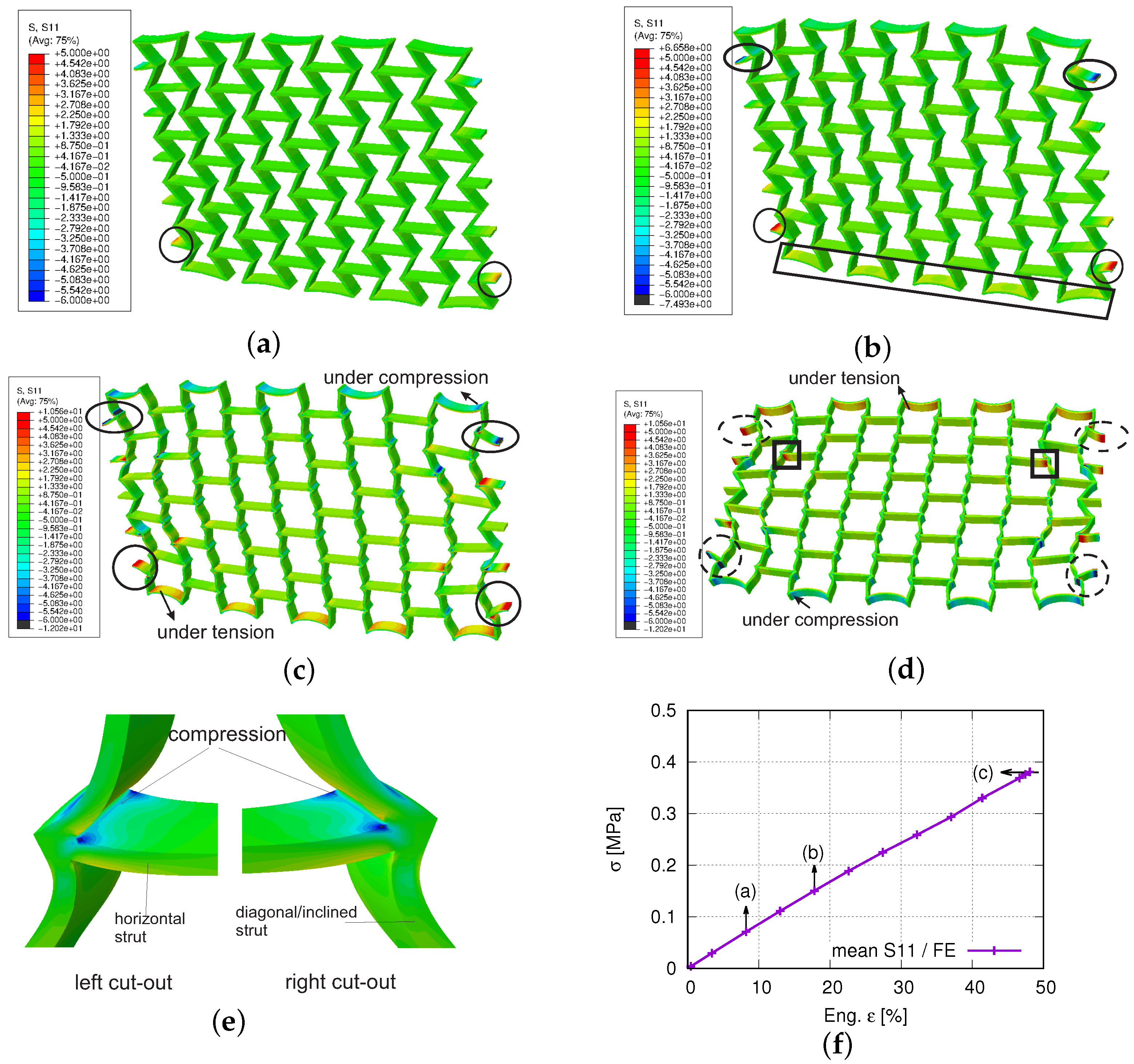
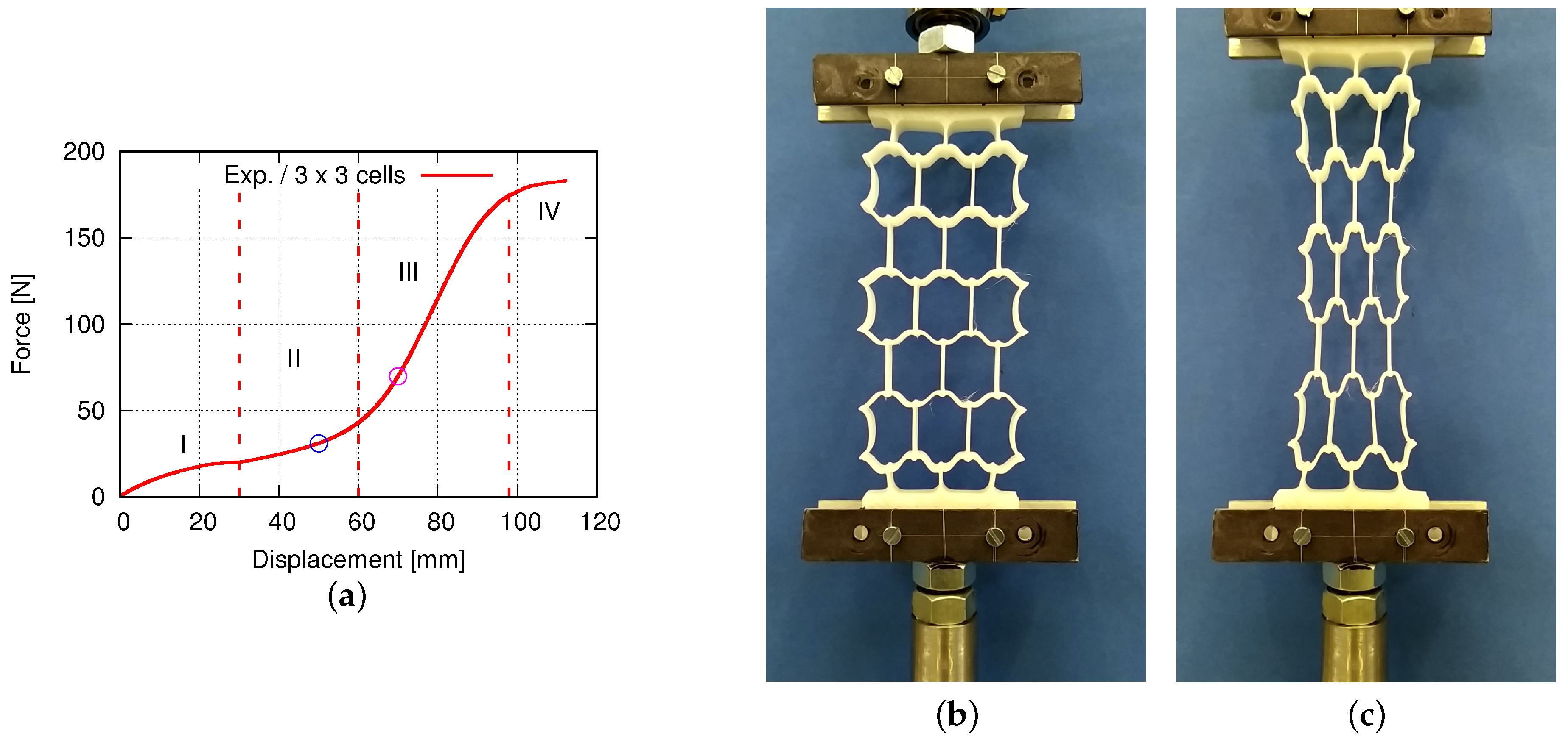
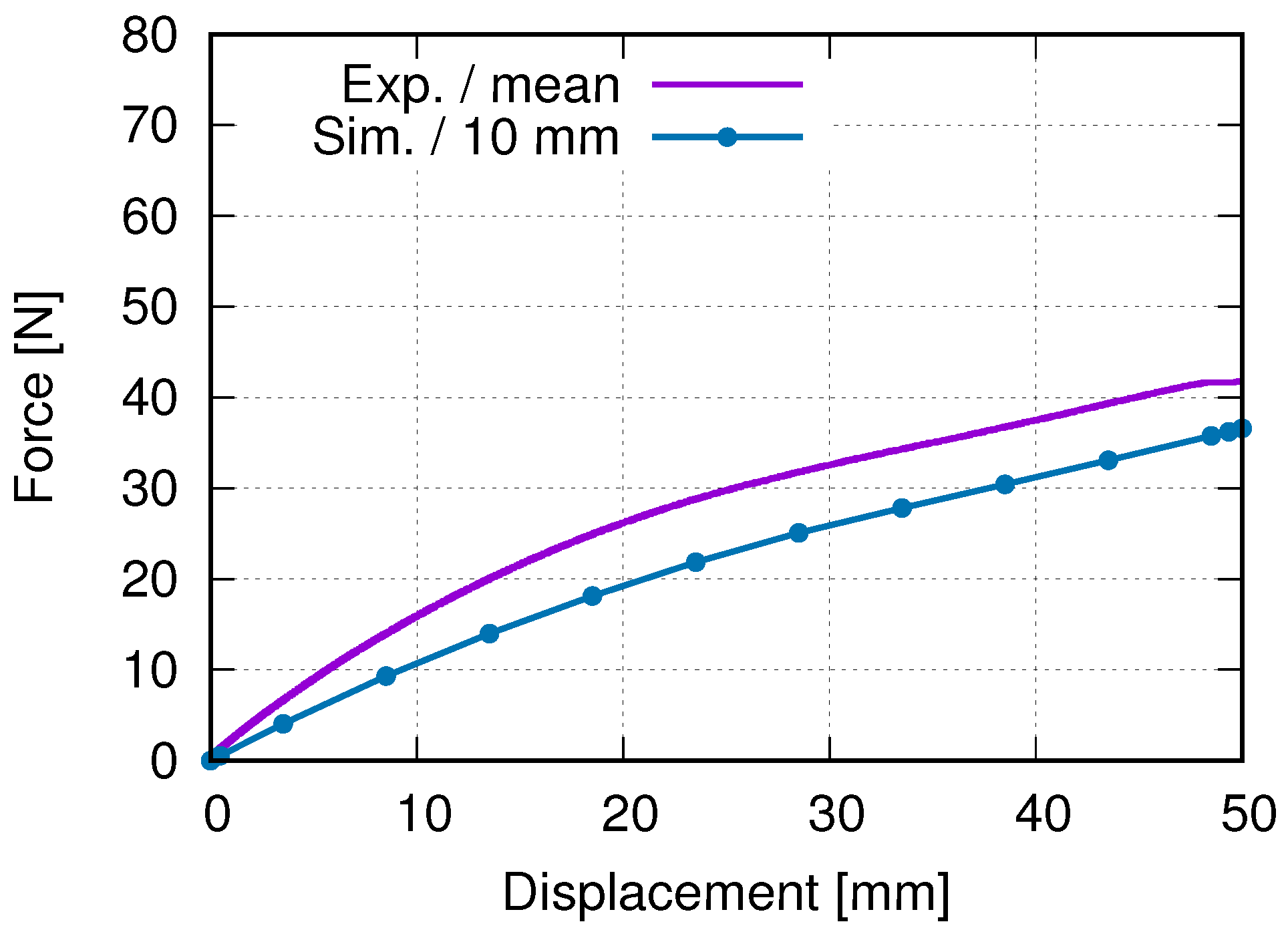
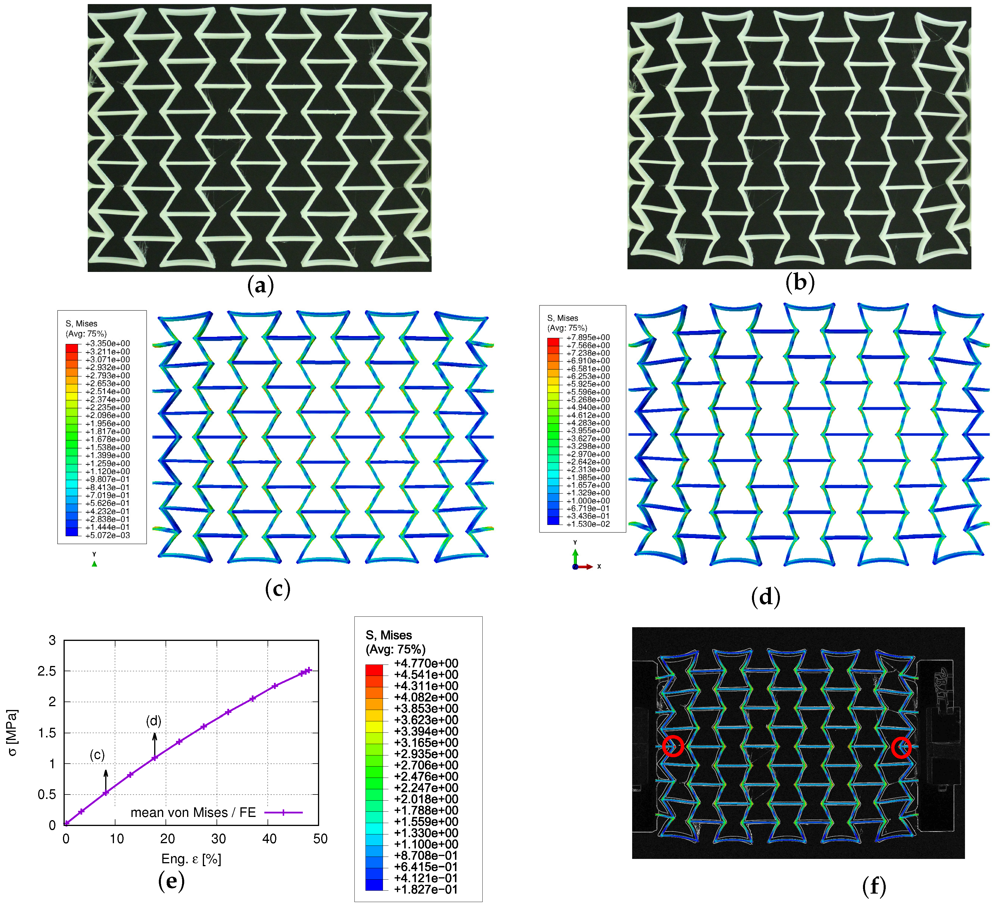
4. Measured and Simulated Results
5. Discussion
6. Conclusions
Author Contributions
Funding
Institutional Review Board Statement
Informed Consent Statement
Data Availability Statement
Conflicts of Interest
References
- Evans, K.E. Auxetic polymers: A new range of materials. Endeavour 1991, 15, 170–174. [Google Scholar] [CrossRef]
- Wojciechowski, K. Remarks on “Poisson Ratio beyond the Limits of the Elasticity Theory”. J. Phys. Soc. Jpn. 2003, 72, 1819–1820. [Google Scholar] [CrossRef]
- Landau, L. Theory of Elasticity, 3rd ed.; Pergamon Press: Oxford, UK, 1993. [Google Scholar]
- Ren, X.; Das, R.; Tran, P.; Ngo, T.; Xie, Y. Auxetic metamaterials and structures: A review. Smart Mater. Struct. 2018, 27, 023001. [Google Scholar] [CrossRef]
- Grima, J.; Gatt, R. Perforated Sheets Exhibiting Negative Poisson’s Ratios. Adv. Eng. Mater. 2010, 12, 460–464. [Google Scholar] [CrossRef]
- Almgren, R. An isotropic three-dimensional structure with Poisson’s ratio = −1. J. Elast. 1985, 15, 427–430. [Google Scholar] [CrossRef]
- Ai, L.; Gao, X.L. Metamaterials with negative Poisson’s ratio and non-positive thermal expansion. Compos. Struct. 2017, 162, 70–84. [Google Scholar] [CrossRef] [Green Version]
- Pandini, S.; Pegoretti, A. Time and temperature effects on Poisson’s ratio of poly(butylene terephthalate). eXPRESS Polym. Lett. 2011, 5, 685–697. [Google Scholar] [CrossRef]
- Gibson, L.J.; Ashby, M.; Schajer, G.S.; Robertson, C.I. The mechanics of two-dimensional cellular materials. Proc. R. Soc. Lond. A 1982, 382, 25–42. [Google Scholar] [CrossRef]
- Wang, Z.; Luan, C.; Liao, G.; Liu, J.; Yao, X.; Fu, J. Progress in Auxetic Mechanical Metamaterials: Structures, Characteristics, Manufacturing Methods, and Applications. Adv. Eng. Mater. 2020, 22, 2000312. [Google Scholar] [CrossRef]
- Yang, H.; Wang, B.; Ma, L. Mechanical properties of 3D double-U auxetic structures. Int. J. Solids Struct. 2019, 180–181, 13–29. [Google Scholar] [CrossRef]
- Orhan, S.; Erden, S. Numerical Investigation of the Mechanical Properties of 2D and 3D Auxetic Structures. Smart Mater. Struct. 2022, 31, 065011. [Google Scholar] [CrossRef]
- Kim, Y.; Son, K.H.; Lee, J.W. Auxetic Structures for Tissue Engineering Scaffolds and Biomedical Devices. Materials 2021, 14, 6821. [Google Scholar] [CrossRef] [PubMed]
- Gohar, S.; Hussain, G.; Ilyas, M.; Ali, A. Performance of 3D printed topologically optimized novel auxetic structures under compressive loading: Experimental and FE analyses. J. Mater. Res. Technol. 2021, 15, 394–408. [Google Scholar] [CrossRef]
- Mercer, C.; Speck, T.; Lee, J.; Balint, D.S.; Thielen, M. Effects of geometry and boundary constraint on the stiffness and negative Poisson’s ratio behaviour of auxetic metamaterials under quasi-static and impact loading. Int. J. Impact Eng. 2021, 169, 1–12. [Google Scholar] [CrossRef]
- Masselter, T.; Bold, G.; Thielen, M.; Speck, O.; Speck, T. Bioinspired Materials and Structures: A Case Study Based on Selected Examples. In Bioinspired Materials Science and Engineering; Yang, G., Xiao, L., Lamboni, L., Eds.; Wiley: Wuhan, China, 2018; pp. 251–266. [Google Scholar] [CrossRef]
- Bührig-Polaczek, A.; Fleck, C.; Speck, T.; Schüler, P.; Fischer, S.; Caliaro, M.; Thielen, M. Biomimetic cellular metals-using hierarchical structuring for energy absorption. Bioinspir. Biomim. 2016, 11, 045002. [Google Scholar] [CrossRef]
- Choi, S.; Ku, Z.; Kim, S.; Choi, K.; Urbas, A.; Kim, Y. Silk is a natural metamaterial for self-cooling: An oxymoron? In Proceedings of the 2018 Conference on Lasers and Electro-Optics (CLEO), San Jose, CA, USA, 13–18 May 2018; pp. 1–2. [Google Scholar]
- Lakes, R. Foam Structures with a Negative Poisson’s Ratio. Science 1987, 235, 1038–1040. [Google Scholar] [CrossRef] [PubMed]
- Kelkar, P.U.; Kim, H.S.; Cho, K.H.; Kwak, J.Y.; Kang, C.Y.; Song, H.C. Cellular Auxetic Structures for Mechanical Metamaterials: A Review. Sensors 2020, 20, 3132. [Google Scholar] [CrossRef] [PubMed]
- Negrea, R. Brief review of metamaterials and auxetic materials. Automot. Ser. 2021, XXVII, 1–9. [Google Scholar] [CrossRef]
- Jiao, J.; Zeng, X.; Huang, X. An overview on synthesis, properties and applications of poly(butylene-adipate-co-terephthalate)–PBAT. Adv. Ind. Eng. Polym. Res. 2020, 3, 19–26. [Google Scholar] [CrossRef]
- Azevedo, J.V.C.; Dorp, E.R.v.; Hausnerova, B.; Möginger, B. The effects of chain-extending cross-linkers on the mechanical and thermal properties of poly(butylene adipate terephthalate)/Poly(lactic acid) blown films. Polymers 2021, 13, 3092. [Google Scholar] [CrossRef]
- Agaliotis, E.; Ake-Concha, B.; May-Pat, A.; Morales Arias, J.; Bernal, C.; Valadez, A.; Herrera-Franco, P.; Proust, G.; Koh-Dzul, J.; Carrillo, J.; et al. Tensile Behavior of 3D Printed Polylactic Acid (PLA) Based Composites Reinforced with Natural Fiber. Polymers 2022, 14, 3976. [Google Scholar] [CrossRef]
- Garzon-Hernandez, S.; Arias, A.; Garcia-Gonzalez, D. A continuum constitutive model for FDM 3D printed thermoplastics. Compos. Part Eng. 2020, 201, 1–13. [Google Scholar] [CrossRef]
- Srivatsan, T.; Sudarshan, T. Additive Manufacturing: Innovations, Advances, and Applications, 1st ed.; CRC Press: Boca Raton, FL, USA, 2015. [Google Scholar] [CrossRef]
- Ngo, T.D.; Kashani, A.; Imbalzano, G.; Nguyen, K.T.; Hui, D. Additive manufacturing (3D printing): A review of materials, methods, applications and challenges. Compos. Part Eng. 2018, 143, 172–196. [Google Scholar] [CrossRef]
- Praveena, B.; Lokesh, N.; Abdulrajak, B.; Santhosh, N.; Praveena, B.; Vignesh, R. A comprehensive review of emerging additive manufacturing (3D printing technology): Methods, materials, applications, challenges, trends and future potential. Mater. Today Proc. 2022, 52, 1309–1313. [Google Scholar] [CrossRef]
- Manoj Prabhakar, M.; Saravanan, A.; Haiter Lenin, A.; Jerin Leno, I.; Mayandi, K.; Sethu Ramalingam, P. A short review on 3D printing methods, process parameters and materials. Mater. Today Proc. 2021, 45, 6108–6114. [Google Scholar] [CrossRef]
- Lee, C.; Padzil, F.; Lee, S.; Ainun, Z.; Abdullah, L. Potential for Natural Fiber Reinforcement in PLA Polymer Filaments for Fused Deposition Modeling (FDM). Addit. Manuf. Rev. 2021, 13, 1–18. [Google Scholar]
- Bergström, J.; Boyce, M. Constitutive modeling of the large strain time-dependent behavior of elastomers. J. Mech. Phys. Solids 1998, 46, 931–954. [Google Scholar] [CrossRef]
- Bergström, J.; Boyce, M. Large strain time-dependent behavior of filled elastomers. Mech. Mater. 2000, 32, 627–644. [Google Scholar] [CrossRef]
- Bergström, J.; Kurtz, S.; Rimnac, C.; Edidin, A. Constitutive modeling of ultra-high molecular weight polyethylene under large-deformation and cyclic loading conditions. Biomaterials 2002, 23, 2329–2343. [Google Scholar] [CrossRef]
- Bergström, J.; Bischoff, J.E. An advanced thermomechanical constitutive model for UHMWPE. Int. J. Struct. Chang. Solids 2010, 2, 31–39. [Google Scholar]
- Mirkhalaf, S.; Andrade Pires, F.; Simoes, R. An elasto-viscoplastic constitutive model for polymers at finite strains: Formulation and computational aspects. Comput. Struct. 2016, 166, 60–74. [Google Scholar] [CrossRef] [Green Version]
- Govaert, L.E.; Timmermans, P.H.M.; Brekelmans, W.A.M. The Influence of Intrinsic Strain Softening on Strain Localization in Polycarbonate: Modeling and Experimental Validation. J. Eng. Mater. Technol. 2000, 122, 177–185. [Google Scholar] [CrossRef] [Green Version]
- Mirkhalaf, S.; Andrade Pires, F.; Simoes, R. Determination of the size of the Representative Volume Element (RVE) for the simulation of heterogeneous polymers at finite strains. Finite Elem. Anal. Des. 2016, 119, 30–44. [Google Scholar] [CrossRef] [Green Version]
- Mirkhalaf, S.; Andrade Pires, F.; Simoes, R. Modelling of the post yield response of amorphous polymers under different stress states. Int. J. Plast. 2017, 88, 159–187. [Google Scholar] [CrossRef] [Green Version]
- Dal, H.; Kaliske, M. Bergström–Boyce model for nonlinear finite rubber viscoelasticity: Theoretical aspects and algorithmic treatment for the FE method. Comput. Mech. 2009, 44, 809–823. [Google Scholar] [CrossRef]
- Hufert, J.; Grebhardt, A.; Schneider, Y.; Bonten, C.; Schmauder, S. Deformation Behavior of 3D Printed Auxetic Structures of Thermoplast Polyermers: PLA, PBAT, and Blends. Polymers 2023, 15, 389. [Google Scholar] [CrossRef]
- Liu, B.; Guan, T.; Wu, G.; Fu, Y.; Weng, Y. Biodegradation Behavior of Degradable Mulch with Poly (Butylene Adipate-co-Terephthalate) (PBAT) and Poly (Butylene Succinate) (PBS) in Simulation Marine Environment. Polymers 2022, 14, 1515. [Google Scholar] [CrossRef]
- Ferreira, F.; Cividanes, L.; Gouveia, R.; Lona, L. An overview on properties and applications of poly(butylene adipate-co-terephthalate)–PBAT based composites. Polym. Eng. Sci. 2019, 59, E7–E15. [Google Scholar] [CrossRef] [Green Version]
- Jiang, L.; Wolcott, M.P.; Zhang, J. Study of Biodegradable Polylactide/Poly(butylene adipate-co-terephthalate) Blends. Biomacromelecules 2006, 7, 199–207. [Google Scholar] [CrossRef]
- ABAQUS/Standard.; Hibbitt, Karlsson & Sorensen, Inc. 2020. Available online: https://www.3ds.com/products-services/simulia/ (accessed on 5 March 2023).
- ABAQUS/Standard.; Hibbitt, Karlsson & Sorensen, Inc. 2018. Available online: https://www.3ds.com/products-services/simulia/ (accessed on 5 March 2023).
- Sahin, A.O. Finite Element Simulations of Additively Manufactured PBAT Polymer with Auxetic Behavior in 2D and 3D. Master thesis, Nr. 759 292, Institute for Materials Testing, Materials Science and Strength of Materials (IMWF), University of Stuttgart, Stuttgart, Germany, 2022. [Google Scholar]
- Hou, C. Numerical Investigations on Additive Manufacturing of Metamaterials with 2D Structure. Master thesis, Nr. 760 148, Institute for Materials Testing, Materials Science and Strength of Materials (IMWF), University of Stuttgart, Stuttgart, Germany, 2020. [Google Scholar]
- Marlow, R. A general first-invariant hyperelastic constitutive model. In Constitutive Models for Rubber III; Busfield, J., Muhr, A., Eds.; Balkema: Lisse, The Netherlands, 2003; pp. 157–160. [Google Scholar]
- Yeoh, O.; Fleming, P. A new attempt to reconcile the statistical and phenomenological theories of rubber elasticity. J. Polym. Sci. Part Polym. Phys. 1997, 35, 1919–1931. [Google Scholar] [CrossRef]
- Ogden, R. Large deformation isotropic elasticity—On the correlation of theory and experiment for incompressible rubberlike solids. Proc. R. Soc. Lond. A 1972, 326, 565–584. [Google Scholar] [CrossRef]
- ABAQUS/Standard.; Hibbitt, Karlsson & Sorensen, Inc. 2022. Available online: https://www.3ds.com/products-services/simulia/ (accessed on 5 March 2023).
- Hosseini, M.; Ali, A.; Sahari, B. A Review of Constitutive Models for Rubber-Like Materials. Am. J. Eng. Appl. Sci. 2010, 3, 232–239. [Google Scholar]
- Bonten, C. Kunststofftechnik—Einführung und Grundlagen; Hanser: München, Germany, 2016. [Google Scholar]
- Rehau. Materialmerkblatt AV0270, 2019. Company Rehau. Available online: https://www.rehau.com/group-en (accessed on 1 May 2020).
- Digimat AM. 2019. Available online: https://www.e-xstream.com/product/digimat-am (accessed on 17 November 2022).
- Box, F.; Johnson, C.; Pihler-Puzović, D. Hard auxetic metamaterials. Extrem. Mech. Lett. 2020, 40, 100980. [Google Scholar] [CrossRef]
- Xue, Y.; Gao, P.; Zhou, L.; Han, F. An Enhanced Three-Dimensional Auxetic Lattice Structure with Improved Property. Materials 2020, 13, 1008. [Google Scholar] [CrossRef] [PubMed] [Green Version]
- Ulbin, M.; Borovinšek, M.; Vesenjak, M.; Glodež, S. Computational Fatigue Analysis of Auxetic Cellular Structures Made of SLM AlSi10Mg Alloy. Metals 2020, 10, 945. [Google Scholar] [CrossRef]
- Meena, K.; Singamneni, S. A new auxetic structure with significantly reduced stress concentration effects. Mater. Des. 2019, 173, 107779. [Google Scholar] [CrossRef]
- Mauko, A.; Fíla, T.; Falta, J.; Koudelka, P.; Rada, V.; Neuhäuserová, M.; Zlámal, P.; Vesenjak, M.; Jiroušek, O.; Ren, Z. Dynamic Deformation Behaviour of Chiral Auxetic Lattices at Low and High Strain-Rates. Metals 2021, 11, 52. [Google Scholar] [CrossRef]


| Content | Speed | Speed | Distance | Time | |||||||
|---|---|---|---|---|---|---|---|---|---|---|---|
| Symbol | n | v | s | s | s | s | t | t | t | t | t |
| Unit | m/min. | cm | cm | s | |||||||
| PBAT | 7 | 30 | 14.8 | 45 | 11.2 | 4 | 67.61 | 1.15 | 30 | 30 | 9.75 |
| Content | Pressure | Temperature | |||||||||
| Symbol | p | p | p | t | t | t | t | t | t | t | t |
| Unit | bar | C | |||||||||
| PBAT | 824 | 500 | 60 | 50 | 160 | 180 | 185 | 190 | 200 | 40 | 40 |
| n: rotatinal speed of filament screw | v: injection speed | ||||||||||
| s: changeover point | s: metering stroke | ||||||||||
| s: mass cushion | s: decompression | ||||||||||
| t: cycle time | t: injection time | ||||||||||
| t: holding pressure time | t: cooling time | ||||||||||
| t: dosing time | p: injection pressure | ||||||||||
| p: holding pressure | p: back pressure | ||||||||||
| t–t: cylinder temperature 1–5 | t: nozzle tempertature | ||||||||||
| t: mold temperature gate side | t: mold temperature clamping side | ||||||||||
| Printer model: | Prusa i3 MK2 |
| Nozzle diameter: | 0.4 [mm] |
| Extrusion width: | 0.44 [mm] |
| Printing temperature: | 200 [C] |
| Plate temperature: | 60 [C] |
| Layer height: | 0.2 [mm] |
| Print speed: | 35 [mm/s] |
| infill pattern: | triangles (25% infill only in clamping bars) |
| Parameter | Value | Parameter | Value | Parameter | Value |
|---|---|---|---|---|---|
| N | 4 | 0.41 | - | - | |
| : | 5.2798 | −32.7303 | 0.01112 | ||
| : | 5.2803 | 1.7398 | 0.0 | ||
| : | −1.0637 | 3.5032 | 0.0 | ||
| : | −10.5607 | 61.9267 | 0.0 |
Disclaimer/Publisher’s Note: The statements, opinions and data contained in all publications are solely those of the individual author(s) and contributor(s) and not of MDPI and/or the editor(s). MDPI and/or the editor(s) disclaim responsibility for any injury to people or property resulting from any ideas, methods, instructions or products referred to in the content. |
© 2023 by the authors. Licensee MDPI, Basel, Switzerland. This article is an open access article distributed under the terms and conditions of the Creative Commons Attribution (CC BY) license (https://creativecommons.org/licenses/by/4.0/).
Share and Cite
Schneider, Y.; Guski, V.; Schmauder, S.; Kadkhodapour, J.; Hufert, J.; Grebhardt, A.; Bonten, C. Deformation Behavior Investigation of Auxetic Structure Made of Poly(butylene adipate-co-terephthalate) Biopolymers Using Finite Element Method. Polymers 2023, 15, 1792. https://doi.org/10.3390/polym15071792
Schneider Y, Guski V, Schmauder S, Kadkhodapour J, Hufert J, Grebhardt A, Bonten C. Deformation Behavior Investigation of Auxetic Structure Made of Poly(butylene adipate-co-terephthalate) Biopolymers Using Finite Element Method. Polymers. 2023; 15(7):1792. https://doi.org/10.3390/polym15071792
Chicago/Turabian StyleSchneider, Yanling, Vinzenz Guski, Siegfried Schmauder, Javad Kadkhodapour, Jonas Hufert, Axel Grebhardt, and Christian Bonten. 2023. "Deformation Behavior Investigation of Auxetic Structure Made of Poly(butylene adipate-co-terephthalate) Biopolymers Using Finite Element Method" Polymers 15, no. 7: 1792. https://doi.org/10.3390/polym15071792
APA StyleSchneider, Y., Guski, V., Schmauder, S., Kadkhodapour, J., Hufert, J., Grebhardt, A., & Bonten, C. (2023). Deformation Behavior Investigation of Auxetic Structure Made of Poly(butylene adipate-co-terephthalate) Biopolymers Using Finite Element Method. Polymers, 15(7), 1792. https://doi.org/10.3390/polym15071792