
A Novel Multi-Region, Multi-Phase, Multi-Component-Mixture Modeling Approach to Predicting the Thermodynamic Behaviour of Thermoplastic Composites during the Consolidation Process


 ,
,
Abstract
1. Introduction
2. Modeling
2.1. Theoretical Background
2.1.1. Basic Equations
2.1.2. Boundary Conditions
2.2. Simulation Studies
2.2.1. Sensitivity Study
2.2.2. Mesh Study
2.2.3. Validation Study
3. Results
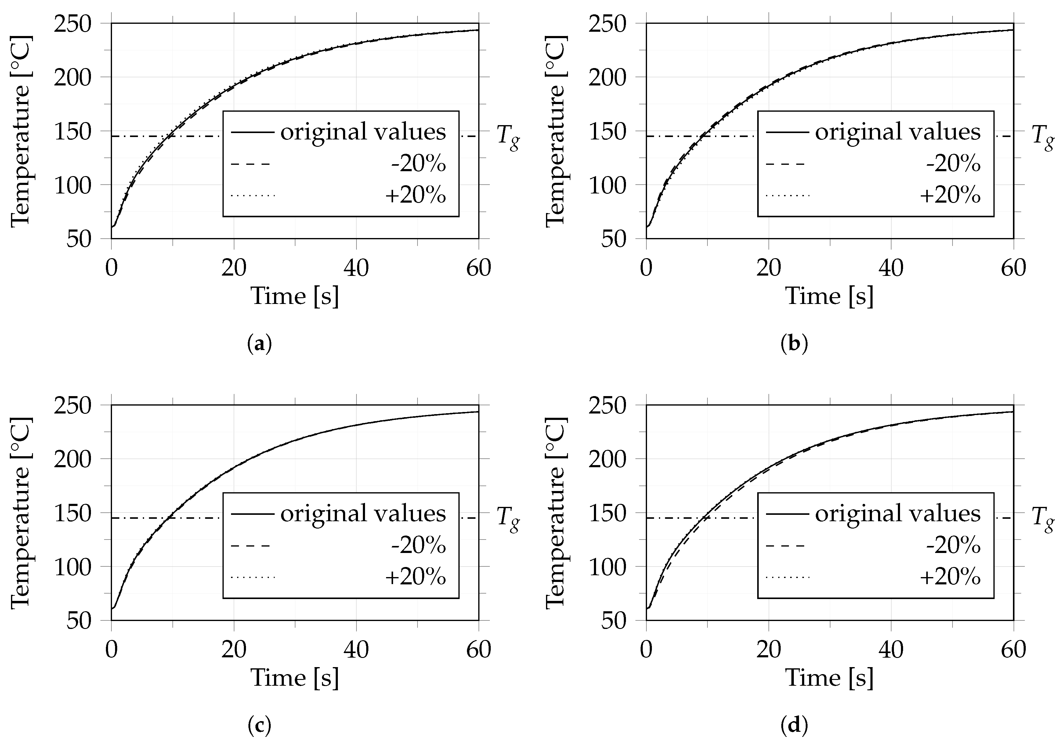
3.1. Model Sensitivity to Changes in Thermal Material Properties
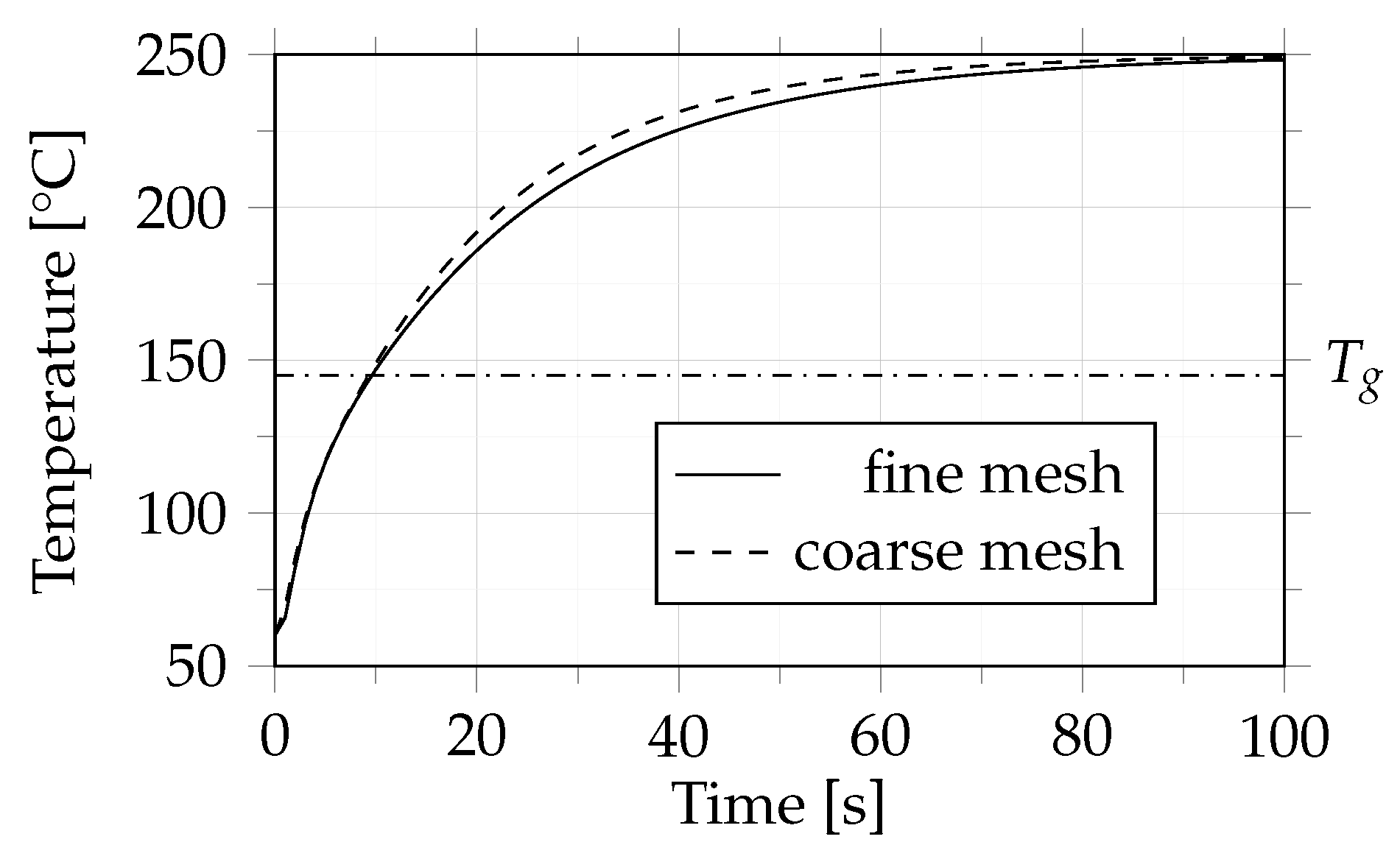
3.2. Mesh Study
3.3. Parameter Study
3.3.1. Case 1
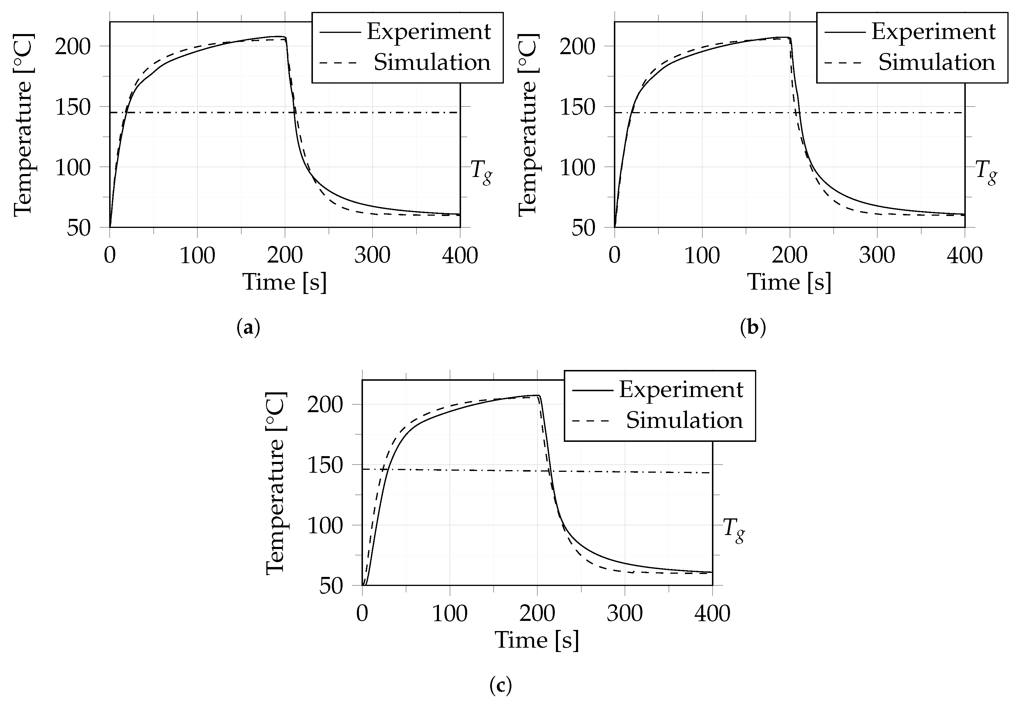
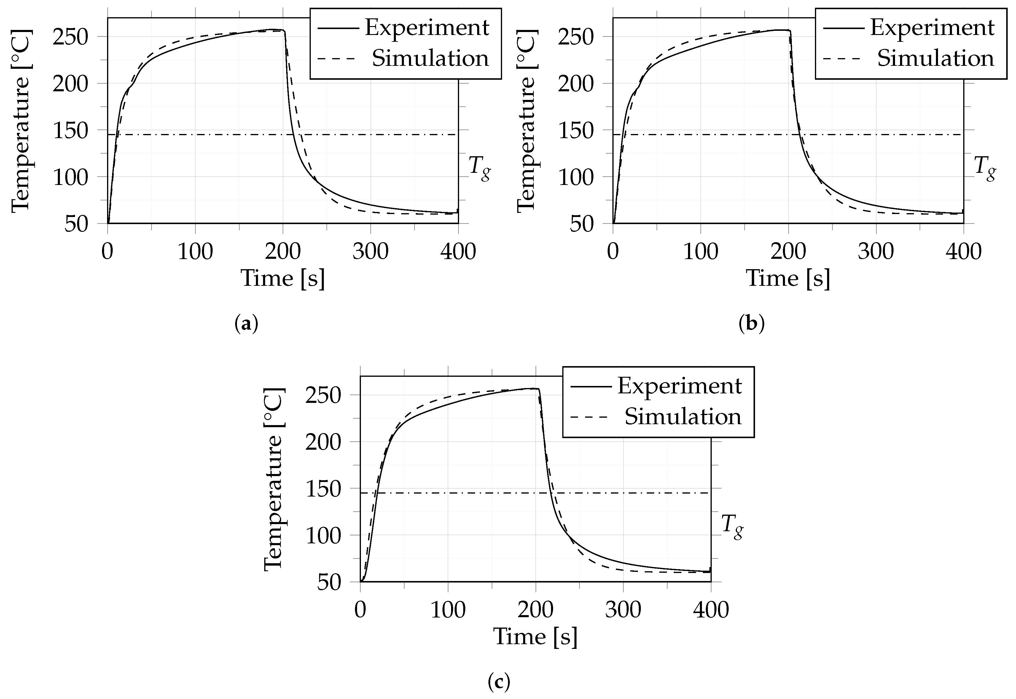
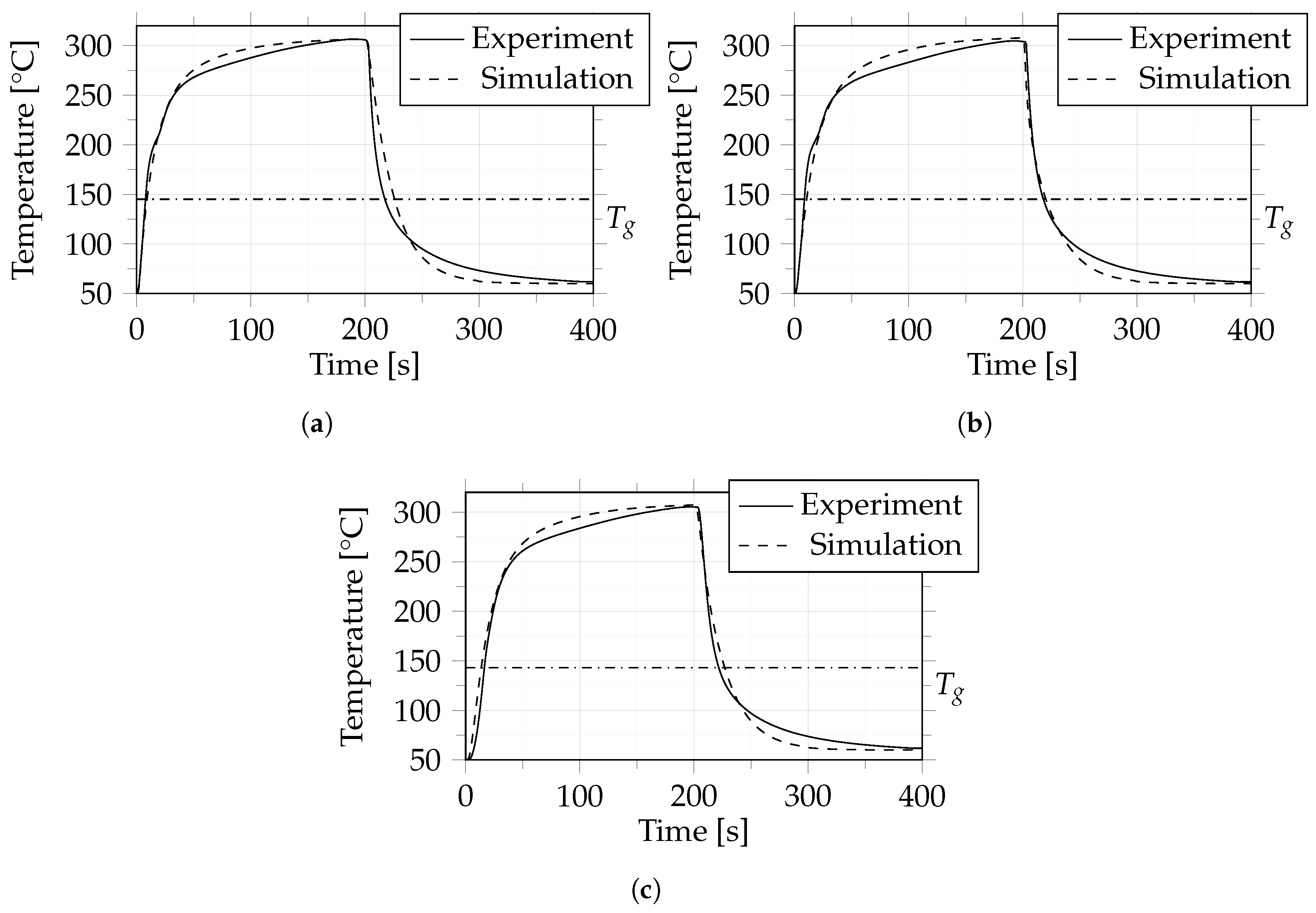
3.3.2. Cases 2, 3 and 4
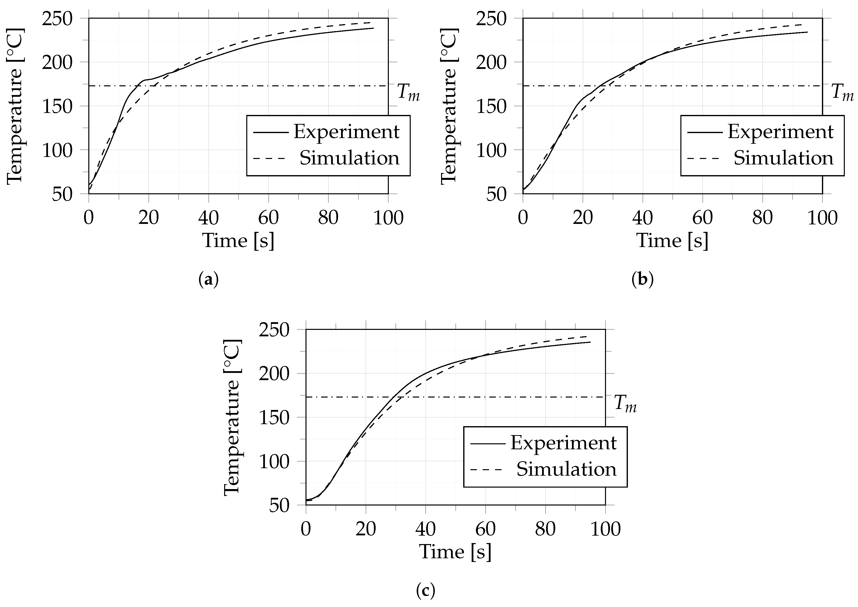
3.3.3. Case 5
4. Discussion and Conclusions
Author Contributions
Funding
Institutional Review Board Statement
Informed Consent Statement
Data Availability Statement
Acknowledgments
Conflicts of Interest
Abbreviations
| AFP | Automated fiber placement |
| ATL | Automated tape laying |
| ILSS | Interlaminar shear strength |
| CFD | Computational fluid dynamics |
References
- Vaidya, U.K.; Chawla, K.K. Processing of fibre reinforced thermoplastic composites. Int. Mater. Rev. 2008, 53, 158–218. [Google Scholar] [CrossRef]
- Das, S.; Graziano, D.; Upadhyayula, V.K.K.; Masanet, E.; Riddle, M.; Cresko, J. Vehicle lightweighting energy use impacts in U.S. light-duty vehicle fleet. Sustain. Mater. Technol. 2016, 8, 5–13. [Google Scholar] [CrossRef]
- Amasawa, E.; Mikiaki Hasegawa, M.; Yokokawa, N.; Sugiyama, H.; Hirao, M. Environmental performance of an electric vehicle composed of 47% polymers and polymer composites. Sustain. Mater. Technol. 2020, 25, e00189. [Google Scholar] [CrossRef]
- Ghosh, T.; Kim, H.C.; De Kleine, R.; Wallington, T.; Bakshi, B.R. Life cycle energy and greenhouse gas emissions implications of using carbon fiber reinforced polymers in automotive components: Front subframe case study. Sustain. Mater. Technol. 2021, 28, e00263. [Google Scholar] [CrossRef]
- Kulshreshtha, A.K.; Vasile, C. Handbook of Polymer Blends and Composites, 1st ed.; Smithers Rapra Publishing: Shrewsbury, UK, 2002. [Google Scholar]
- Krawczak, P.; Maffezzoli, A. Editorial: Advanced Thermoplastic Composites and Manufacturing Processes. Front. Mater. 2020, 7, 166. [Google Scholar] [CrossRef]
- Proja, J. Composite Materials in the Airbus A380 -From History to Future-. In Proceedings of the International Conference of Composite Materials-13, Beijing, China, 25–29 June 2001; p. 1695. [Google Scholar]
- Gardiner, G. Thermoplastic composites gain leading edge on the A380. High-Perform. Compos. 2014, 14, 50–55. [Google Scholar]
- Yousefpour, A.; Hojjati, M.; Immarigeon, J.-P. Fusion Bonding/Welding of Thermoplastic Composites. Thermoplast. Compos. Mater. 2004, 17. [Google Scholar] [CrossRef]
- Benatar, A.; Gutowski, T.G. Methods for Fusion Bonding Thermoplastic Composites. SAMPE Quaterly 1986, 18, 35–42. [Google Scholar]
- Todd, S.M. Joining Thermoplastic Composites. In Proceedings of the 22nd International SAMPE Technical Conference, Boston, MA, USA, 6–8 November 1990; pp. 383–392. [Google Scholar]
- Stokes, V.K. Joining Methods for Plastics and Plastic Composites: An Overview. Polym. Eng. Sci. 1989, 29, 1310–1324. [Google Scholar] [CrossRef]
- Bourban, P.-E.; Bernet, N.; Zanetto, J.-E.; Manson, J.-A. Material phenomena controlling rapid processing of thermoplastic composites. Compos. Part Appl. Sci. Manuf. 2001, 32, 1045–1057. [Google Scholar] [CrossRef]
- JEC Group JEC Observer—Press Kit—March 2022. Paris March 2022. Available online: https://www.jeccomposites.com/wp-content/uploads/2022/03/V1_14588_DP-Digital-JEC-_VERSION_COMPOSITE_2022_02_24.pdf (accessed on 11 May 2022).
- Thermoplastic Composites Market: Global Industry Trends, Share, Size, Growth, Opportunity and Forecast 2022–2027. Available online: https://www.imarcgroup.com/thermoplastic-composites-market (accessed on 11 May 2022).
- Thermoplastic Composites Market Outlook—2020–2027. Available online: https://www.alliedmarketresearch.com/thermoplastic-composites-market-A11057 (accessed on 11 May 2022).
- Henning, F.; Möller, E. Faserverstärkte Kunststoffe. In Handbuch Leichtbau: Methoden, Werkstoffe, Fertigung, 2nd ed.; Carl Hanser Verlag: Munich, Germany, 2020; pp. 339–381. [Google Scholar]
- Henning, F.; Möller, E. Fertigungstechnologien für faserverstärkte Kunststoffe. In Handbuch Leichtbau: Methoden, Werkstoffe, Fertigung, 2nd ed.; Carl Hanser Verlag: Munich, Germany, 2020; pp. 569–631. [Google Scholar]
- Slange, T.K. Rapid Manufacturing of Tailored Thermoplastic Composites by Automated Lay-Up and Stamp Forming–A Study on the Consolidation Mechanisms. Ph.D. Thesis, University of Twente, Twente, The Netherlands, 2019. [Google Scholar]
- Brzeski, M. Experimental and Analytical Investigation of Deconsolidation for Fiber Reinforced Thermoplastic Composites. Ph.D. Thesis, TU Kaiserslautern, Kaiserslautern, Germany, 2014. [Google Scholar]
- Slange, T.C.; Warnet, L.; Grouve, W.J.B.; Akkerman, R. Influence of preconsolidation on consolidation quality after stamp forming of C/PEEK composites. In Proceedings of the 19th International ESAFORM Conference on Material Forming, Nantes, France, 27–29 April 2016. [Google Scholar]
- Donough, M.J.; Shafaq; St John, N.A.; Philips, A.W.; Prusty, B.G. Process modelling of In-situ consolidated thermoplastic composite by automated fibre placement–A review. Compos. Part Appl. Sci. Manuf. 2022, 163, 107179. [Google Scholar] [CrossRef]
- Weller, H.G. A New Approach to VOF-Based Interface Capturing Methods for Incompressible and Compressible Flow; Report TR/HGW 4; OpenCFD Ltd.: Bracknell, UK, 2008; Volume 35. [Google Scholar]
- Lee, D.G.; Jeong, M.Y.; Choi, J.H.; Cheon, S.S.; Oh, J.H. Composite Materials; Hongrung Publishing Company: Seoul, Korea, 2007; pp. 173–176. [Google Scholar]
- Mantell, S.; Wang, Q.; Springer, G.S. Processing Thermoplastic Composites in a Press and by Tape Laying–Experimental Results. J. Compos. Mater. 1992, 26, 2378–2401. [Google Scholar] [CrossRef]
- Lee, W.I.; Springer, G.E. A Model of the Manufacturing Process of Thermoplastic Matrix Composites. J. Compos. Mater. 1987, 21. [Google Scholar] [CrossRef]
- Guglhör, T. Experimentelle und Modellhafte Betrachtung des Konsolidierungsprozesses von Carbonfaserverstärktem Polyamid-6. Ph.D. Thesis, Universität Augsburg, Augsburg, Germany, 2017. [Google Scholar]
- Khan, M.A.; Mitschang, P.; Schledjewski, R. Identification of some optimal parameters to achieve higher laminate quality through tape placement process. Adv. Polym. Technol. 2010, 29, 100. [Google Scholar] [CrossRef]
- Khan, M.A.; Mitschang, P.; Schledjewski, R. Parametric study on processing parameters and resulting part quality through thermoplastic tape placement process. J. Compos. Mater. 2012, 47, 485–499. [Google Scholar] [CrossRef]
- Tierney, J.; Gillespie, J.W. Modeling of In Situ Strength Development for the Thermoplastic Composite Tow Placement Process. J. Compos. Mater. 2006, 40, 1487–1506. [Google Scholar] [CrossRef]
- Levy, A.; Heider, D.; Tierney, J.; Gillespie, J.W. Inter-layer thermal contact resistance evolution with the degree of intimate contact in the processing of thermoplastic composite laminates. J. Compos. Mater. 2014, 48, 491–503. [Google Scholar] [CrossRef]
- Schledjewski, R.; Latrille, M. Processing of unidirectional fiber reinforced tapes-fundamentals on the way to a process simulation tool (ProSimFRT). Compos. Sci. Technol. 2003, 63, 2111–2118. [Google Scholar] [CrossRef]
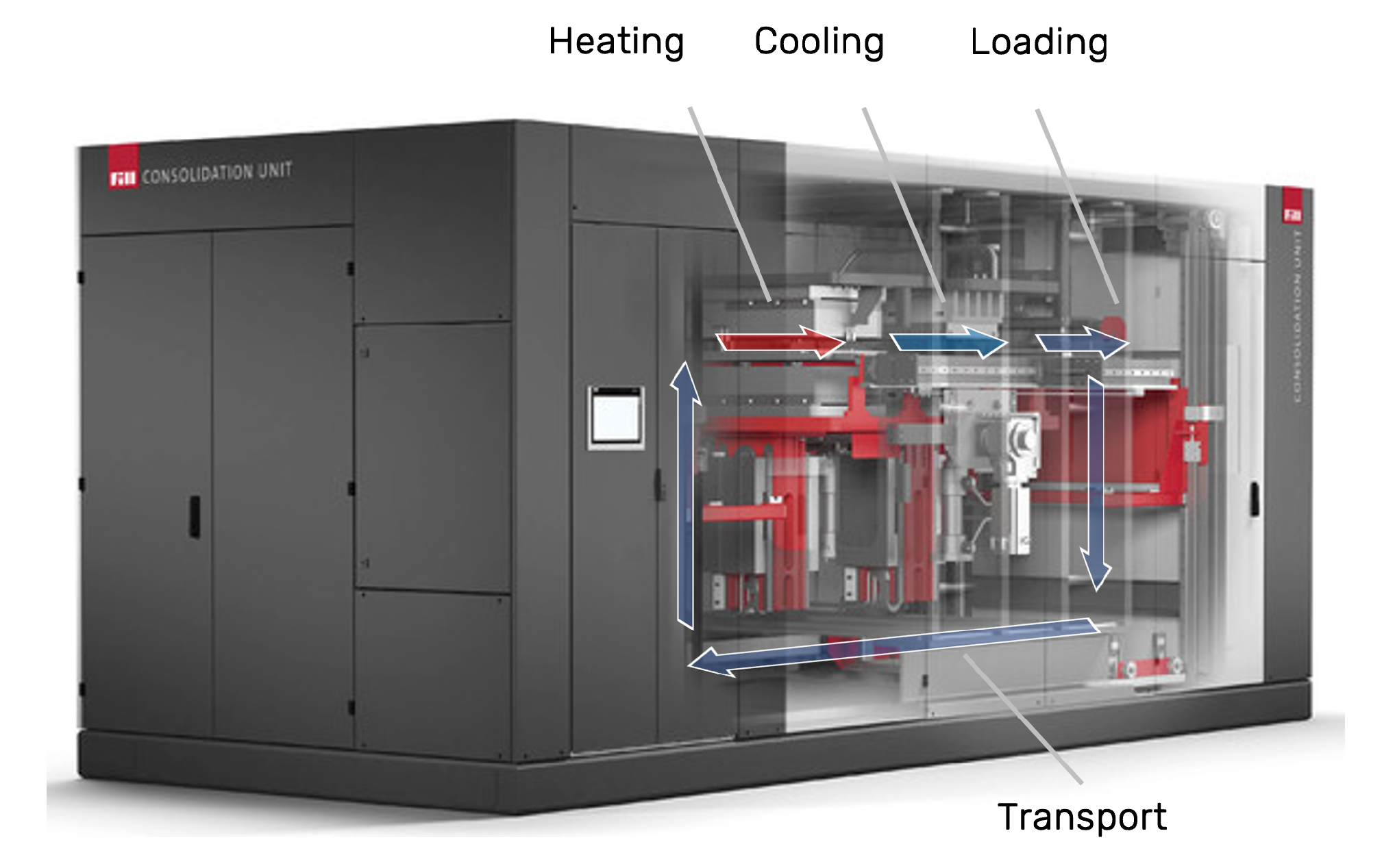
- Consolidation Unit. Available online: https://www.fill.co.at (accessed on 10 November 2021).


| Parameter | Source | Value |
|---|---|---|
| specific heat capacity matrix | measured | polynomial fit |
| specific heat capacity fiber | litaerature | 1200 J/(kg K) |
| specific heat capacity mixture | measured + Equation (9) | polynomial fit |
| thermal conductivity matrix | literature | 0.2 W/(m K) |
| thermal conductivity fiber | literature | 0.5 W/(m K) |
| thermal conductivity mixture | Equation (9) | 0.332 W/(m K) |
| density matrix | measured | polynomial fit |
| density fiber | literature | 1790 kg/m3 |
| density mixture | Equation (9) | polynomial fit |
| dynamic viscosity matrix | measured | polynomial fit |
| dynamic viscosity fiber | Equation (9) | 2.3 × 10⁶ Pa s |
| dynamic viscosity mixture | measured | polynomial fit |
| Original Value | −20% | +20% | |
|---|---|---|---|
| specific heat capacity matrix | 1700 J/(kg K) | 1360 J/(kg K) | 2040 J/(kg K) |
| specific heat capacity fiber | 1200 J/(kg K) | 960 J/(kg K) | 1440 J/(kg K) |
| thermal conductivity matrix | 0.2 W/(m K) | 0.16 W/(m K) | 0.24 W/(m K) |
| thermal conductivity fiber | 0.5 W/(m K) | 0.4 W/(m K) | 0.6 W/(m K) |
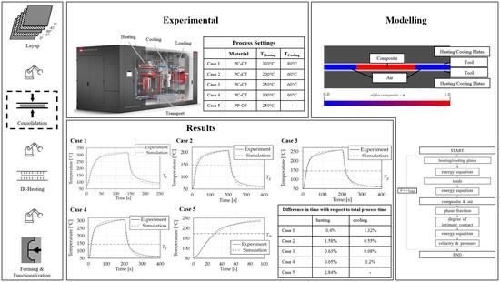
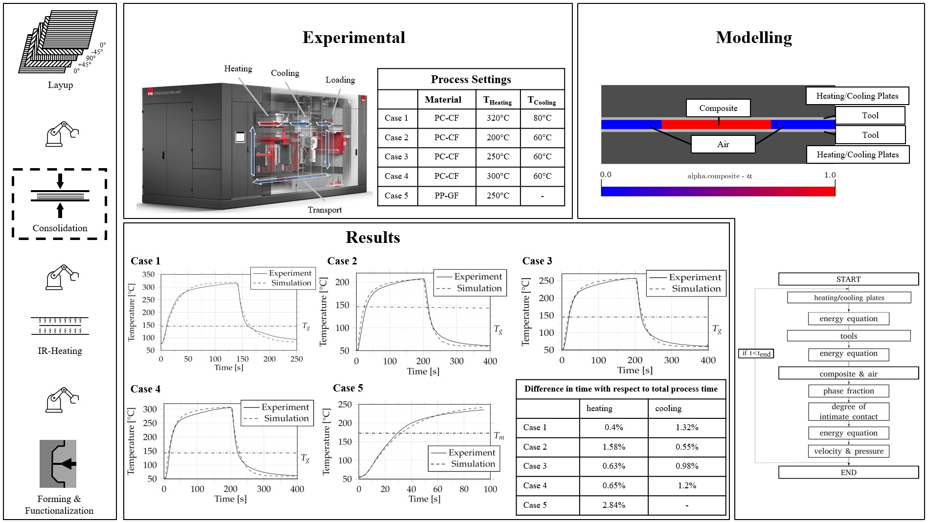
| Material | Layup | TH | TC | pH | pC | tH | tC | |
|---|---|---|---|---|---|---|---|---|
| Case 1 | PC-CF | 2 Sheet Layers | 320 °C | 80 °C | 1 bar | 10 bar | 140 s | 110 s |
| Case 2 | PC-CF | 18 Tape Layers | 200 °C | 60 °C | 1 bar | 30 bar | 200 s | 200 s |
| Case 3 | PC-CF | 18 Tape Layers | 250 °C | 60 °C | 1 bar | 30 bar | 200 s | 200 s |
| Case 4 | PC-CF | 18 Tape Layers | 300 °C | 60 °C | 1 bar | 30 bar | 200 s | 200 s |
| Case 5 | PP-GF | 10 Tape Layers | 250 °C | – | 1 bar | – | 95 s | – |
| Time- Experiment | Time- Simulation | Absolute Difference | Difference with Respect to Total Process Time | |
|---|---|---|---|---|
| Case 2—heating | 29.3 s | 23 s | 6.3 s | 1.58% |
| Case 2—cooling | 215.2 s | 213 s | 2.2 s | 0.55% |
| Case 3—heating | 19.5 s | 17 s | 2.5 s | 0.63% |
| Case 3—cooling | 217.1 s | 221 s | 3.9 s | 0.98% |
| Case 4—heating | 16.6 s | 14 s | 2.6 s | 0.65% |
| Case 4—cooling | 221.1 s | 226 s | 4.8 s | 1.2% |
Publisher’s Note: MDPI stays neutral with regard to jurisdictional claims in published maps and institutional affiliations. |
© 2022 by the authors. Licensee MDPI, Basel, Switzerland. This article is an open access article distributed under the terms and conditions of the Creative Commons Attribution (CC BY) license (https://creativecommons.org/licenses/by/4.0/).
Share and Cite
Kobler, E.; Birtha, J.; Marschik, C.; Straka, K.; Steinbichler, G.; Zwicklhuber, P.; Schlecht, S. A Novel Multi-Region, Multi-Phase, Multi-Component-Mixture Modeling Approach to Predicting the Thermodynamic Behaviour of Thermoplastic Composites during the Consolidation Process. Polymers 2022, 14, 4785. https://doi.org/10.3390/polym14214785
Kobler E, Birtha J, Marschik C, Straka K, Steinbichler G, Zwicklhuber P, Schlecht S. A Novel Multi-Region, Multi-Phase, Multi-Component-Mixture Modeling Approach to Predicting the Thermodynamic Behaviour of Thermoplastic Composites during the Consolidation Process. Polymers. 2022; 14(21):4785. https://doi.org/10.3390/polym14214785
Chicago/Turabian StyleKobler, Eva, Janos Birtha, Christian Marschik, Klaus Straka, Georg Steinbichler, Paul Zwicklhuber, and Sven Schlecht. 2022. "A Novel Multi-Region, Multi-Phase, Multi-Component-Mixture Modeling Approach to Predicting the Thermodynamic Behaviour of Thermoplastic Composites during the Consolidation Process" Polymers 14, no. 21: 4785. https://doi.org/10.3390/polym14214785
APA StyleKobler, E., Birtha, J., Marschik, C., Straka, K., Steinbichler, G., Zwicklhuber, P., & Schlecht, S. (2022). A Novel Multi-Region, Multi-Phase, Multi-Component-Mixture Modeling Approach to Predicting the Thermodynamic Behaviour of Thermoplastic Composites during the Consolidation Process. Polymers, 14(21), 4785. https://doi.org/10.3390/polym14214785