
Optimization of Glass Transition Temperature and Pot Life of Epoxy Blends Using Response Surface Methodology (RSM)


 ,
,  ,
,  and
and
Abstract
:
1. Introduction
2. Materials and Methods
2.1. Epoxy Resin
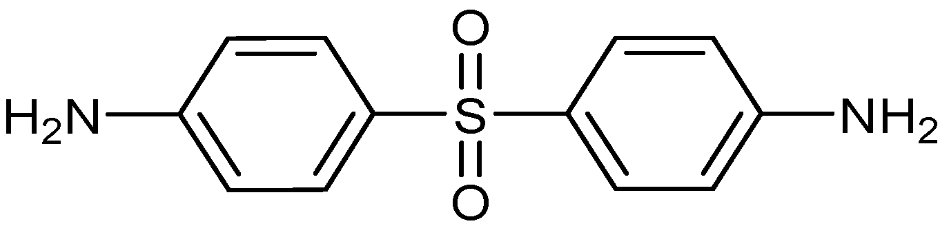
2.2. Hardener
2.3. Resin Mixtures
2.4. Design of Experiment
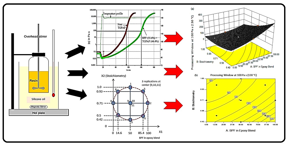
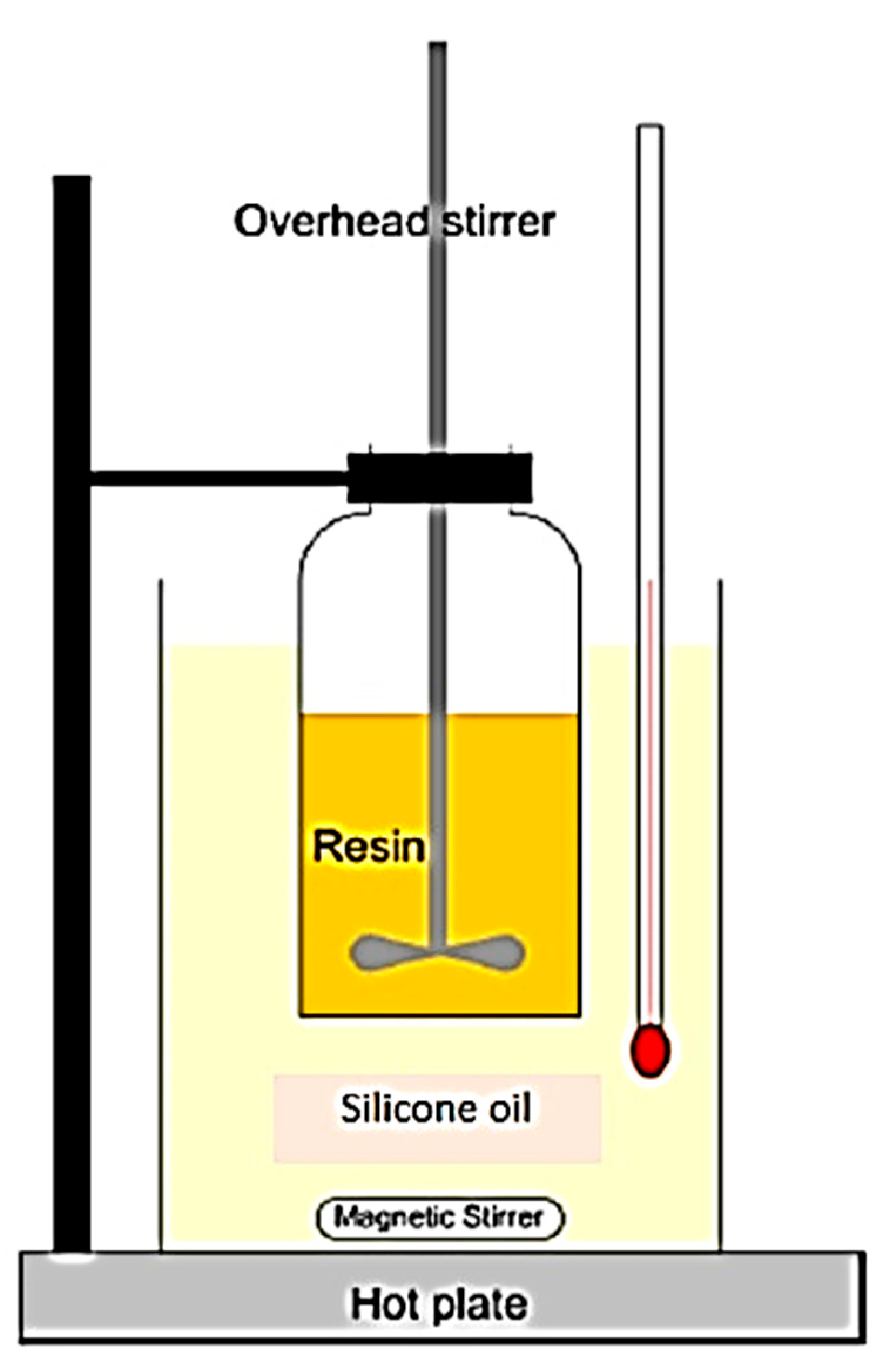
2.5. Testing Procedures
3. Results
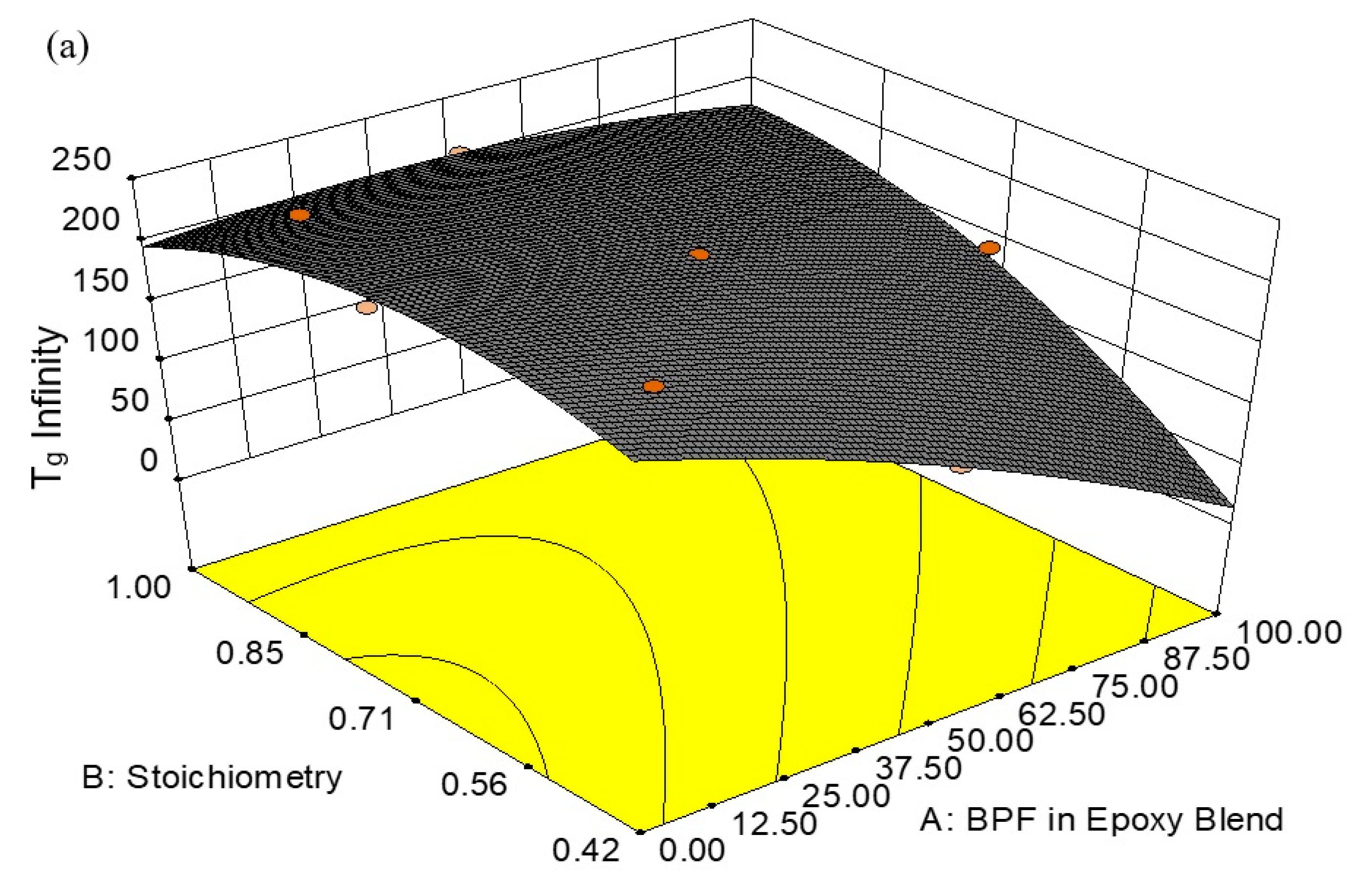
3.1. Glass Transition Temperature
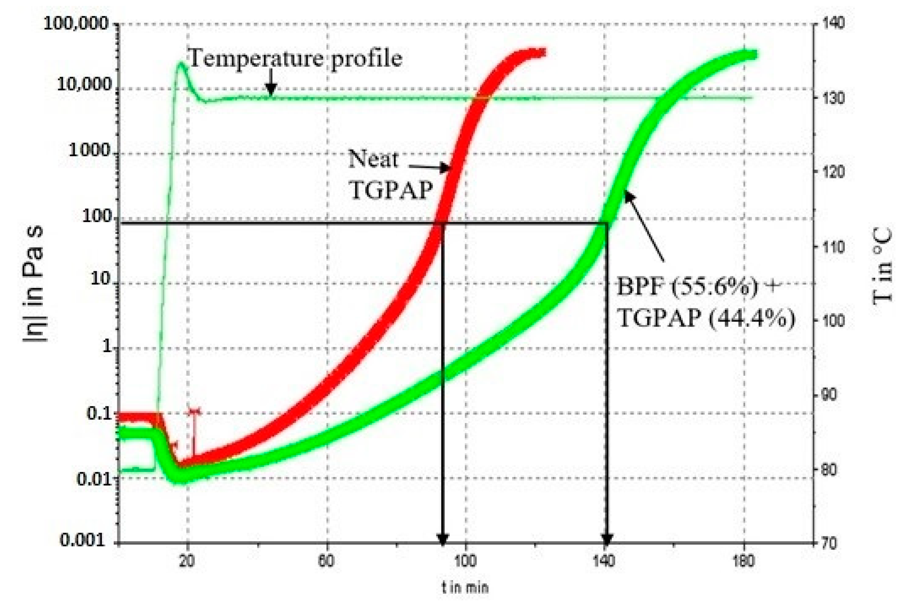
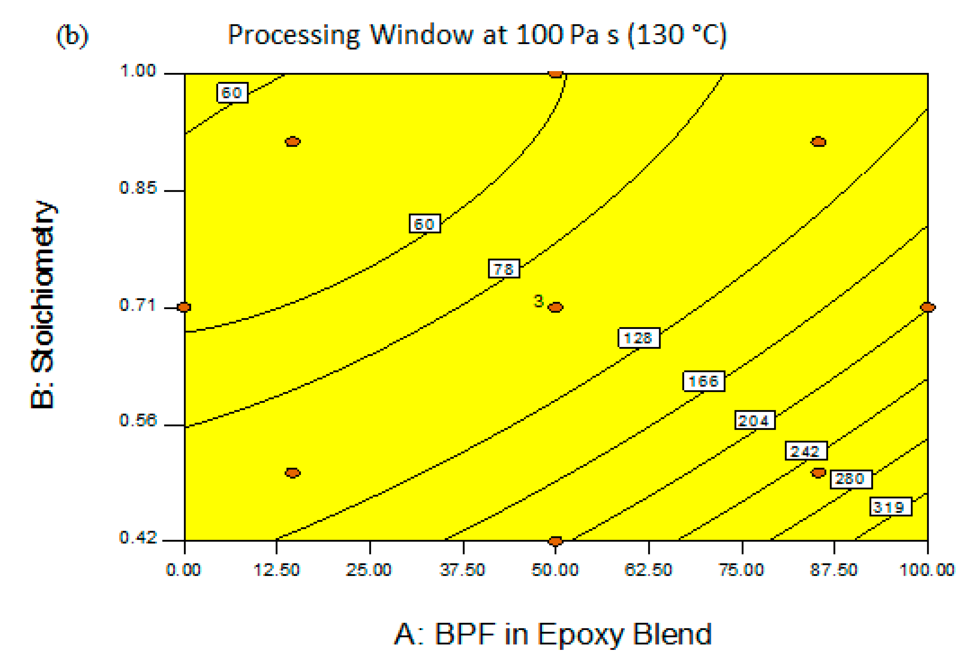
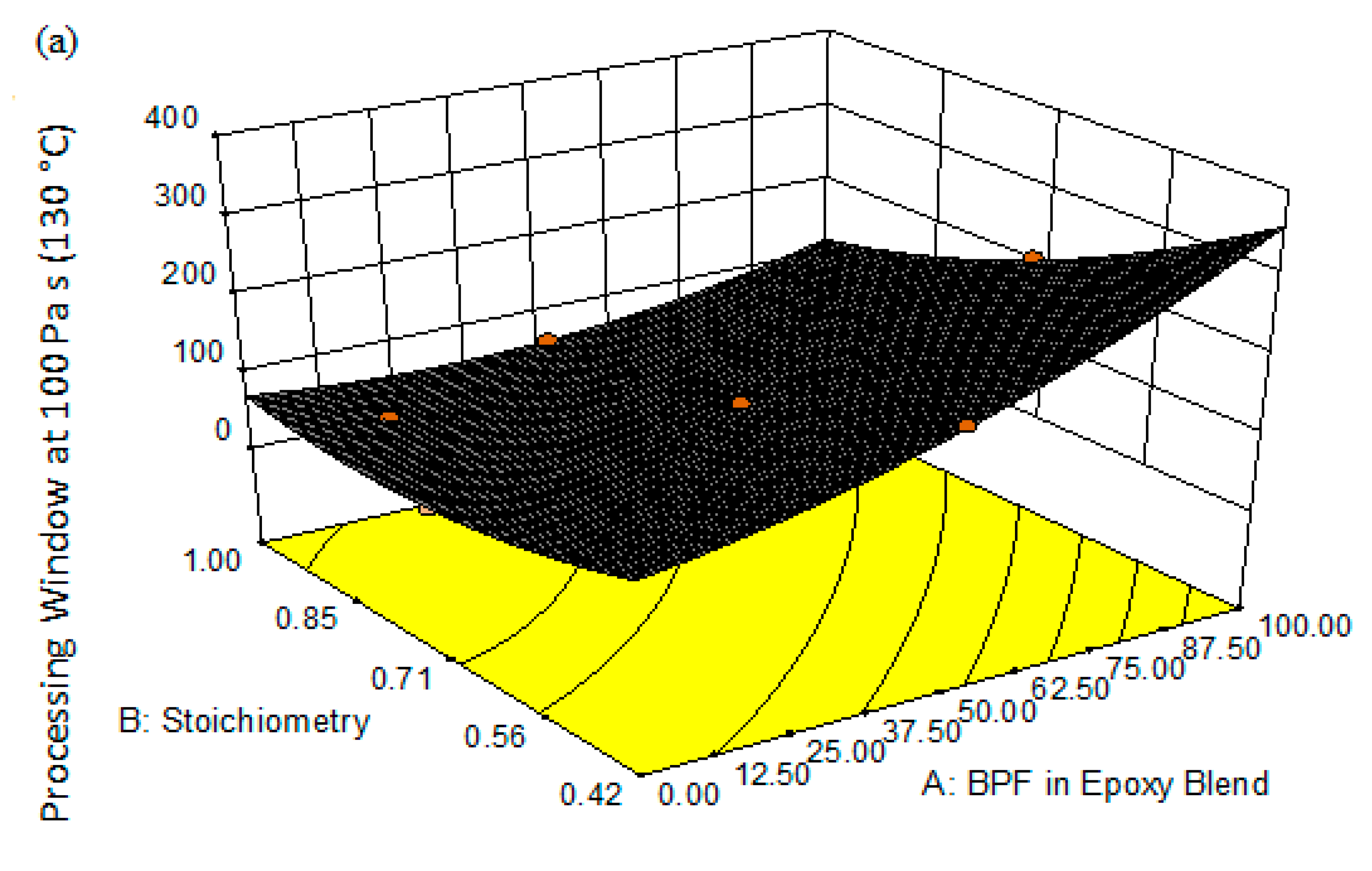
3.2. Pot Life (Processing Window, PW)
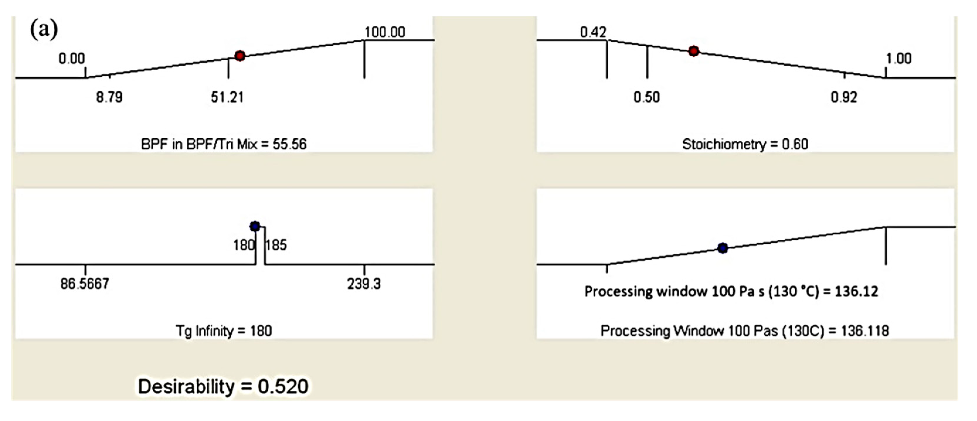
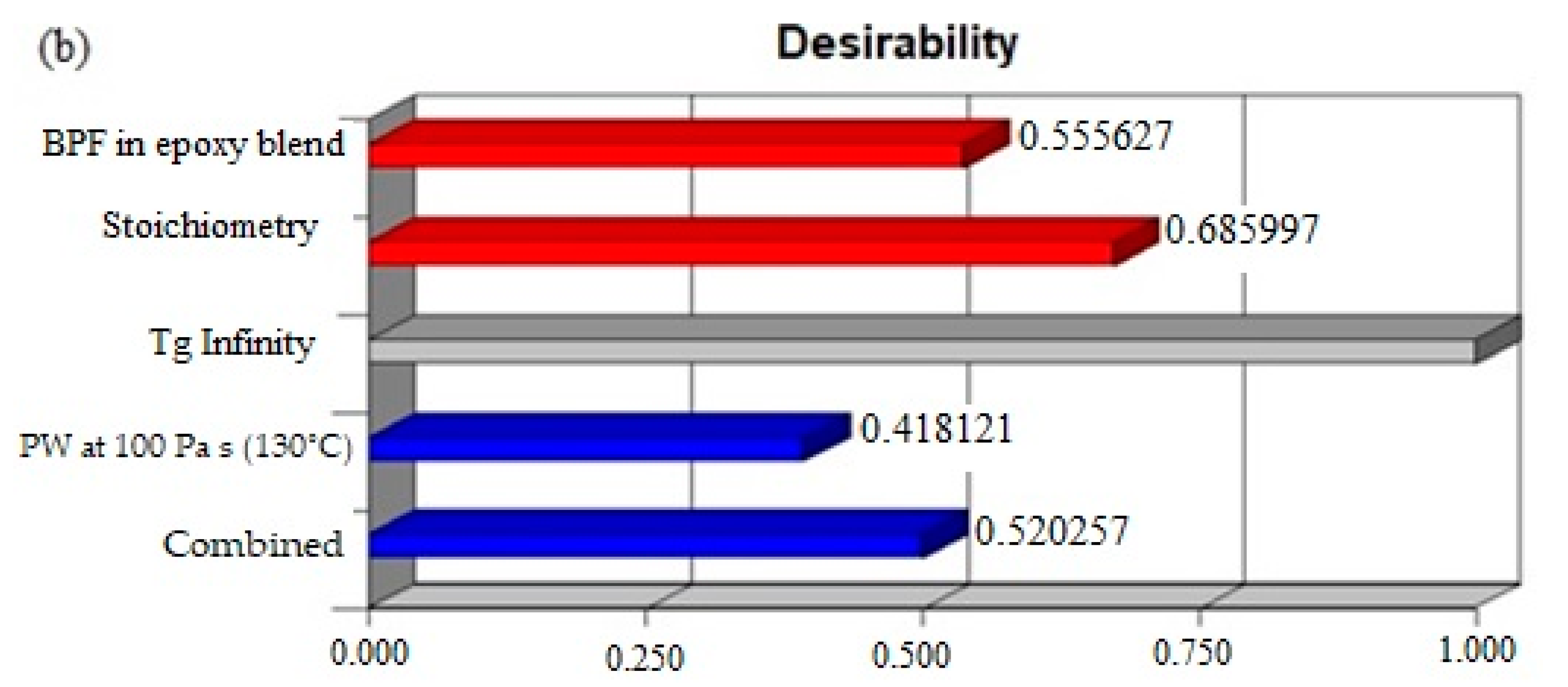
3.3. Optimization of Epoxy Formulation
4. Conclusions
Author Contributions
Funding
Institutional Review Board Statement
Informed Consent Statement
Data Availability Statement
Acknowledgments
Conflicts of Interest
References
- Noor, N.; Razak, J.; Ismail, S.; Mohamad, N.; Junid, R. Review on Carbon Nanotube based Polymer Composites and Its Applications. J. Adv. Manuf. Technol. 2018, 12, 311–326. [Google Scholar]
- Bakar, N.A.; Zulkarnain, M.A.; Hassan, W.A.W.; Junid, R.; Razak, J.A.; Ismail, M.M. The effect of graphite flakes (GFs) and hybrid graphene nanoplatelets (GNPs) particles to the mechanical properties of epoxy composites. In Proceedings of the IOP Conference Series: Materials Science and Engineering; IOP Publishing Ltd.: Bristol, UK, 2020; Volume 957, p. 012033. [Google Scholar]
- Ramli, J.; Jeefferie, A.R.; Mahat, M.M. Effects of uv curing exposure time to the mechanical And physical properties of the epoxy and vinyl ester Fiber glass laminates composites. ARPN J. Eng. Appl. Sci. 2011, 6, 104–109. [Google Scholar]
- Hadi, A.E.; Hamdan, M.H.M.; Siregar, J.P.; Junid, R.; Tezara, C.; Irawan, A.P.; Fitriyana, D.F.; Rihayat, T. Application of Micromechanical Modelling for the Evaluation of Elastic Moduli of Hybrid Woven Jute–Ramie Reinforced Unsaturated Polyester Composites. Polymers 2021, 13, 2572. [Google Scholar] [CrossRef] [PubMed]
- Barde, Y.D.; Ramezanian, N.; Nazif, A.; Behzadpour, M. Effect of Different Diluents on the Main Properties of the Epoxy-Based Composite. J. Mater. Sci. Appl. 2020, 4, 1–9. [Google Scholar] [CrossRef]
- Penn, L.S.; Wang, H. Epoxy Resins. In Handbook of Composites; Springer: Boston, MA, USA, 1998; pp. 48–74. ISBN 978-1-4615-6389-1. [Google Scholar]
- Pham, H.Q.; Marks, M.J. Epoxy resins. Ullmann’s Encycl. Ind. Chem. 2012, 156–238. [Google Scholar] [CrossRef]
- Gibson, G. Epoxy Resins. In Brydson’s Plastics Materials, 8th ed.; Gilbert, M., Ed.; Butterworth-Heinemann Elsevier: Amsterdam, The Netherlands, 2017; pp. 773–797. ISBN 9780323370226. [Google Scholar]
- Varma, I.K.; Gupta, V.B.; Sini, N.K. 2.19 Thermosetting Resin—Properties. Compr. Compos. Mater. 2018, 2, 401–468. [Google Scholar] [CrossRef]
- Ozeren Ozgul, E.; Ozkul, M.H. Effects of epoxy, hardener, and diluent types on the workability of epoxy mixtures. Constr. Build. Mater. 2018, 158, 369–377. [Google Scholar] [CrossRef]
- Qian, J.W.; Miao, Y.M.; Zhang, L.; Chen, H.L. Influence of viscosity slope coefficient of CA and its blends in dilute solutions on permeation flux of their films for MeOH/MTBE mixture. J. Memb. Sci. 2002, 203, 167–173. [Google Scholar] [CrossRef]
- Montserrat, S.; Andreu, G.; Corts, P.; Calventus, Y.; Colomer, P.; Hutchinson, J.M.; Malek, J. Addition of a reactive diluent to a catalyzed epoxy-anhydride system. I. Influence on the cure kinetics. J. Appl. Polym. Sci. 1996, 61, 1663–1674. [Google Scholar] [CrossRef]
- Nikolic, G.; Zlatkovic, S.; Cakic, M.; Cakic, S.; Lacnjevac, C.; Rajic, Z. Fast Fourier Transform IR Characterization of Epoxy GY Systems Crosslinked with Aliphatic and Cycloaliphatic EH Polyamine Adducts. Sensors 2010, 10, 684–696. [Google Scholar] [CrossRef]
- Otter, C.; Stephenson, K. Amines and Amides. In Salters Advanced Chemistry: Chemical Ideas; Heinemann: Portsmouth, NH, USA, 2008; p. 320. [Google Scholar]
- Everitt, D.T.; Luterbacher, R.; Coope, T.S.; Trask, R.S.; Wass, D.F.; Bond, I.P. Optimisation of epoxy blends for use in extrinsic self-healing fibre-reinforced composites. Polymer 2015, 69, 283–292. [Google Scholar] [CrossRef]
- Frank, K.; Childers, C.; Dutta, D.; Gidley, D.; Jackson, M.; Ward, S.; Maskell, R.; Wiggins, J. Fluid uptake behavior of multifunctional epoxy blends. Polymer 2013, 54, 403–410. [Google Scholar] [CrossRef]
- Mason, R.; Gunst, R.; Hess, J. Statistical Design and Analysis of Experiments with Applications to Engineering and Science, 2nd ed.; John Wiley & Sons: New York, NY, USA, 2003. [Google Scholar]
- Mehmood, T.; Ramzan, M.; Howari, F.; Kadry, S.; Chu, Y.-M. Application of response surface methodology on the nanofluid flow over a rotating disk with autocatalytic chemical reaction and entropy generation optimization. Sci. Rep. 2021, 111, 1–18. [Google Scholar] [CrossRef]
- Montgomery, D.C. Design and Analysis of Experiments, 6th ed.; Wiley International Edition: Hoboken, NJ, USA, 2005. [Google Scholar]
- Kasina, M.M.; Joseph, K.; John, M.; Kasina, M.M.; Joseph, K.; John, M. Application of Central Composite Design to Optimize Spawns Propagation. Open J. Optim. 2020, 9, 47–70. [Google Scholar] [CrossRef]
- Guo, J.L.; Guo, W.Y.; Xie, R.J.; Li, Y.M.; Yang, Y.B. Influence of the Additives on the Workability and Mechanic Properties of Epoxy Mortar. Adv. Mater. Res. 2010, 168–170, 2003–2007. [Google Scholar] [CrossRef]
- Harani, H.; Fellahi, S.; Bakar, M. Toughening of epoxy resin using hydroxyl-terminated polyesters. J. Appl. Polym. Sci. 1999, 71, 29–38. [Google Scholar] [CrossRef]
- Plastics, D. Epoxy Resin. Available online: http://nmt.edu/academics/mtls/faculty/mccoy/docs2/chemistry/DowEpoxyResins.pdf (accessed on 24 September 2021).
- ASTM Standard D4473; 95a Standard Test Method for Plastics: Dynamic Mechanical Properties: Cure Behavior; ASTM International: West Conshohocken, PA, USA, 2001.
- Gude, M.R.; Prolongo, S.G.; Ureña, A. Effect of the epoxy/amine stoichiometry on the properties of carbon nanotube/epoxy composites. J. Therm. Anal. Calorim. 2011, 108, 717–723. [Google Scholar] [CrossRef]
- Calventus, Y.; Montserrat, S.; Hutchinson, J.M. Enthalpy relaxation of non-stoichiometric epoxy-amine resins. Polymer 2001, 42, 7081–7093. [Google Scholar] [CrossRef]
- Palmese, G.R.; McCullough, R.L. Effect of epoxy–amine stoichiometry on cured resin material properties. J. Appl. Polym. Sci. 1992, 46, 1863–1873. [Google Scholar] [CrossRef]
- Guerrero, P.; De la Caba, K.; Valea, A.; Corcuera, M.A.; Mondragon, I. Influence of cure schedule and stoichiometry on the dynamic mechanical behaviour of tetrafunctional epoxy resins cured with anhydrides. Polymer 1996, 37, 2195–2200. [Google Scholar] [CrossRef]
- Mohamad, N. Development of Epoxidised Natural Rubber-Alumina Composites (ENRAN) for the Absorption of Ballistic Impact Energy in Body Armour; National University of Malaysia: Bangi, Selangor, Malaysia, 2011. [Google Scholar]
- Response Surface. Available online: https://www.statease.com/docs/v11/tutorials/multifactor-rsm/ (accessed on 14 September 2021).
- Noordin, M.Y.; Venkatesh, V.C.; Sharif, S.; Elting, S.; Abdullah, A. Application of response surface methodology in describing the performance of coated carbide tools when turning AISI 1045 steel. J. Mater. Process. Technol. 2004, 145, 46–58. [Google Scholar] [CrossRef] [Green Version]
- Du Prel, J.B.; Hommel, G.; Röhrig, B.; Blettner, M. Confidence interval or p-value?: Part 4 of a series on evaluation of scientific publications. Dtsch. Arztebl. Int. 2009, 106, 335–339. [Google Scholar] [CrossRef] [PubMed]
- Norhazimah, A.H.; Faizal, C.K.M. Optimization Study on Bioethanol Production from the Fermentation of Oil Palm Trunk Sap as Agricultural Waste. In Developments in Sustainable Chemical and Bioprocess Technology; Springer: Berlin/Heidelberg, Germany, 2013; pp. 19–25. [Google Scholar]
- Korbahti, B.K. Optimization of Electrochemical Oxidation of Textile Dye Wastewater Using Response Surface Methodology (RSM). In Survival and Sustainability; Springer: Berlin/Heidelberg, Germany, 2011; pp. 1181–1191. [Google Scholar]
- Capricho, J.C.; Fox, B.; Hameed, N. Multifunctionality in Epoxy Resins. Polym. Rev. 2020, 60, 1–41. [Google Scholar] [CrossRef]
- Razak, J.A.; Ahmad, S.H.; Ratnam, C.T.; Mahamood, M.A.; Yaakub, J.; Mohamad, N. Effects of EPDM- g -MAH compatibilizer and internal mixer processing parameters on the properties of NR/EPDM blends: An analysis using response surface methodology. J. Appl. Polym. Sci. 2015, 132, 1–15. [Google Scholar] [CrossRef]
- Stein, J. Toughening of Highly Crosslinked Epoxy Resin Systems. Ph.D. Thesis, The University of Manchester, Manchester, UK, 2013. [Google Scholar]
- Design-Expert 7.1 User’s Guide. Mixture Design Tutorial (Part 2—Optimization). Available online: https://www.statease.com/docs/v11/tutorials/mixture-designs-2/ (accessed on 25 September 2021).


| Materials | Trade Name | Equivalent Weight (g/eq) | Density (g/cm3) | Supplier |
|---|---|---|---|---|
| Triglycidyl p-aminophenol (TGPAP) | Araldite MY0500 | 101 | 1.21–1.22 | Huntsman |
| Diglycidyl ether of bisphenol F (BPF) | DER 354 | 164 | 1.19 | Dow Chemical |
| 4,4′-diaminodiphenyl sulfones | DDS | 62.08 | 1.36 | Huntsman |
| Run | Factor 1 | Factor 2 | Response 1 | Response 2 |
|---|---|---|---|---|
| A: BPF in BPF/TGPAP (wt.%) | B: Stoichiometry Amine:Epoxy (g/g) | Glass Transition Temperature (Tg) | Processing Window (min) | |
| 1 | 50 | 1 | 203.2 ± 1.5 | 59.6 ± 3.7 |
| 2 | 100 | 0.71 | 141.2 ± 0.6 | 206.8 ± 2.7 |
| 3 | 50 | 0.42 | 134.5 ± 1.0 | 203 ± 1.3 |
| 4 | 0 | 0.71 | 239.3 ± 0.8 | 57.2 ± 3.4 |
| 5 | 85.4 | 0.92 | 183.8 ± 0.2 | 105.9 ± 2.0 |
| 6 | 85.4 | 0.5 | 86.6 ± 1.0 | 251.4 ± 3.0 |
| 7 | 14.6 | 0.5 | 224.9 ± 0.2 | 102.3 ± 1.6 |
| 8 | 14.6 | 0.92 | 226.2 ± 0.5 | 53.3 ± 7.1 |
| 9 | 50 | 0.71 | 206.4 ± 1.0 | 100.9 ± 2.2 |
| 10 | 50 | 0.71 | 206.6 ± 0.7 | 90.7 ± 2.5 |
| 11 | 50 | 0.71 | 206.4 ± 1.0 | 92.2 ± 2.7 |
| Source | Sum of Squares | df | Mean Square | F Value | p-Value (Prob > F) |
|---|---|---|---|---|---|
| Model | 21,837.58 | 5 | 4367.52 | 97.95 | <0.0001 (Significant) |
| A-BPF in BPF/TGPAP | 2730.24 | 1 | 2730.24 | 61.23 | 0.0005 |
| B-Stoichiometry | 580.89 | 1 | 580.89 | 13.03 | 0.0154 |
| AB | 2296.01 | 1 | 2296.01 | 51.49 | 0.0008 |
| A2 | 353.05 | 1 | 353.05 | 7.92 | 0.0374 |
| B2 | 1960.37 | 1 | 1960.37 | 43.96 | 0.0012 |
| Residual | 222.92 | 5 | 44.59 | ||
| Std. Dev. | 6.68 | R2 | 0.9899 | ||
| Mean | 187.19 | Adj. R2 | 0.9798 | ||
| C. V. % | 3.57 | Pred R2 | 0.9281 | ||
| PRESS | 1585.26 | Adeq. Precision | 31.541 |
| Source | Sum of Squares | df | Mean Square | F Value | p-Value (Prob > F) |
|---|---|---|---|---|---|
| Model | 46,138.06 | 5 | 9227.61 | 441.82 | <0.0001 (Significant) |
| A-BPF in BPF/TGPAP | 2811.65 | 1 | 2811.65 | 134.62 | <0.0001 |
| B-Stoichiometry | 6331.62 | 1 | 6331.62 | 303.16 | <0.0001 |
| AB | 2327.10 | 1 | 2327.10 | 111.42 | 0.0001 |
| A2 | 1801.80 | 1 | 1801.80 | 86.27 | 0.0002 |
| B2 | 1727.93 | 1 | 1727.93 | 82.73 | 0.0003 |
| Residual | 104.43 | 5 | 20.89 | ||
| Std. Dev. | 4.57 | R2 | 0.9977 | ||
| Mean | 120.29 | Adj. R2 | 0.9955 | ||
| C. V. % | 3.80 | Pred R2 | 0.9903 | ||
| PRESS | 449.79 | Adeq. Precision | 60.041 |
| Factor/Response | Goal | Lower Limit | Upper Limit | Importance |
|---|---|---|---|---|
| BPF in BPF/TGPAP | Maximize | 0 | 100 | **** |
| Stoichiometry | Minimize | 0.42 | 1 | *** |
| Tg infinity | Is in range | 180 | 185 | ***** |
| Processing window | Maximize | 53.28 | 251.4 | ***** |
Publisher’s Note: MDPI stays neutral with regard to jurisdictional claims in published maps and institutional affiliations. |
© 2021 by the authors. Licensee MDPI, Basel, Switzerland. This article is an open access article distributed under the terms and conditions of the Creative Commons Attribution (CC BY) license (https://creativecommons.org/licenses/by/4.0/).
Share and Cite
Junid, R.; Siregar, J.P.; Endot, N.A.; Razak, J.A.; Wilkinson, A.N. Optimization of Glass Transition Temperature and Pot Life of Epoxy Blends Using Response Surface Methodology (RSM). Polymers 2021, 13, 3304. https://doi.org/10.3390/polym13193304
Junid R, Siregar JP, Endot NA, Razak JA, Wilkinson AN. Optimization of Glass Transition Temperature and Pot Life of Epoxy Blends Using Response Surface Methodology (RSM). Polymers. 2021; 13(19):3304. https://doi.org/10.3390/polym13193304
Chicago/Turabian StyleJunid, Ramli, Januar Parlaungan Siregar, Nor Azam Endot, Jeefferie Abd Razak, and Arthur N. Wilkinson. 2021. "Optimization of Glass Transition Temperature and Pot Life of Epoxy Blends Using Response Surface Methodology (RSM)" Polymers 13, no. 19: 3304. https://doi.org/10.3390/polym13193304
APA StyleJunid, R., Siregar, J. P., Endot, N. A., Razak, J. A., & Wilkinson, A. N. (2021). Optimization of Glass Transition Temperature and Pot Life of Epoxy Blends Using Response Surface Methodology (RSM). Polymers, 13(19), 3304. https://doi.org/10.3390/polym13193304