
Cellular Automata Modeling of Three-Dimensional Chitosan-Based Aerogels Fiberous Structures with Bezier Curves


Abstract
:
1. Introduction
2. Materials and Methods
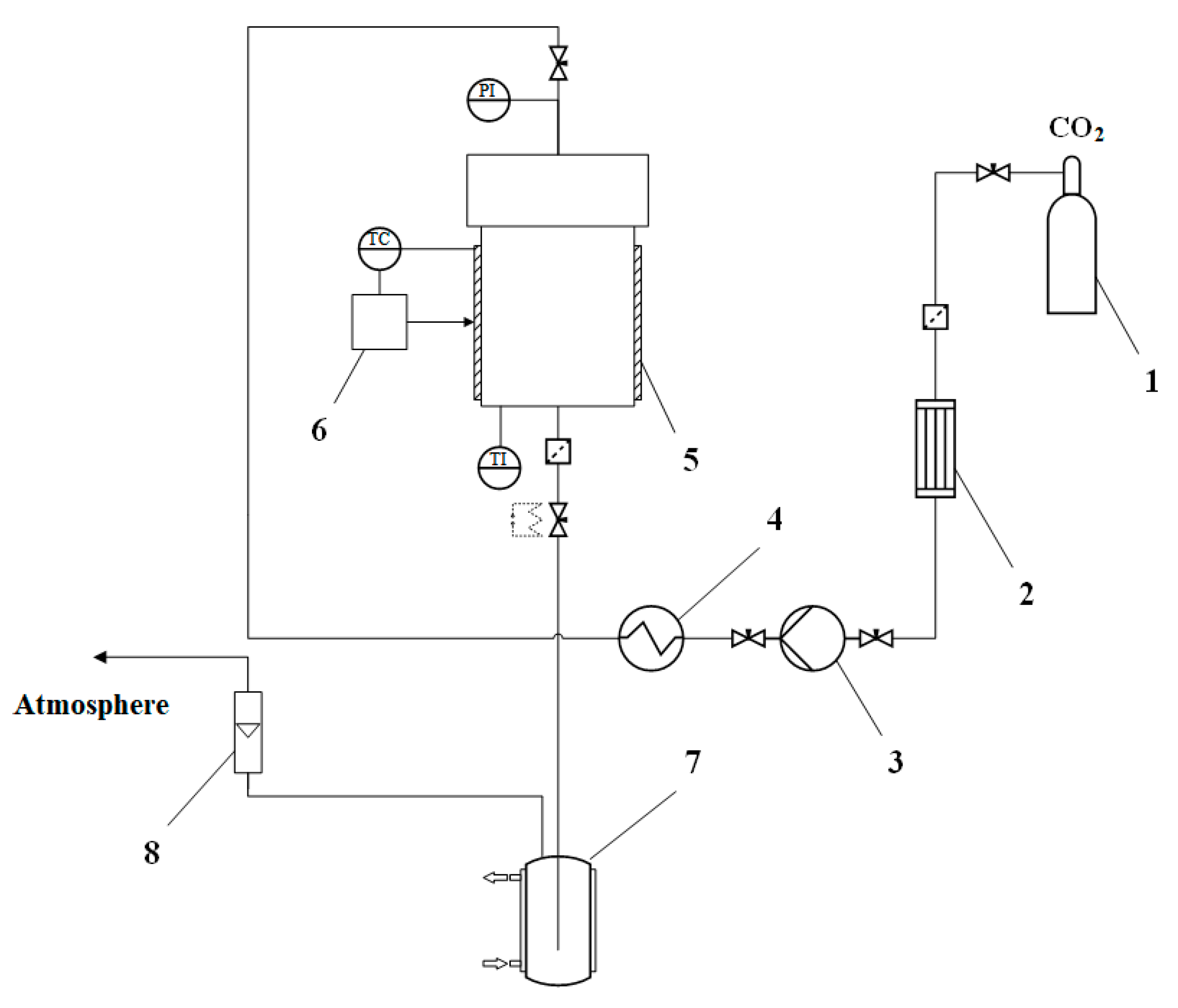
2.1. Synthesis of Chitosan-Based Gel Particles via Dripping Method
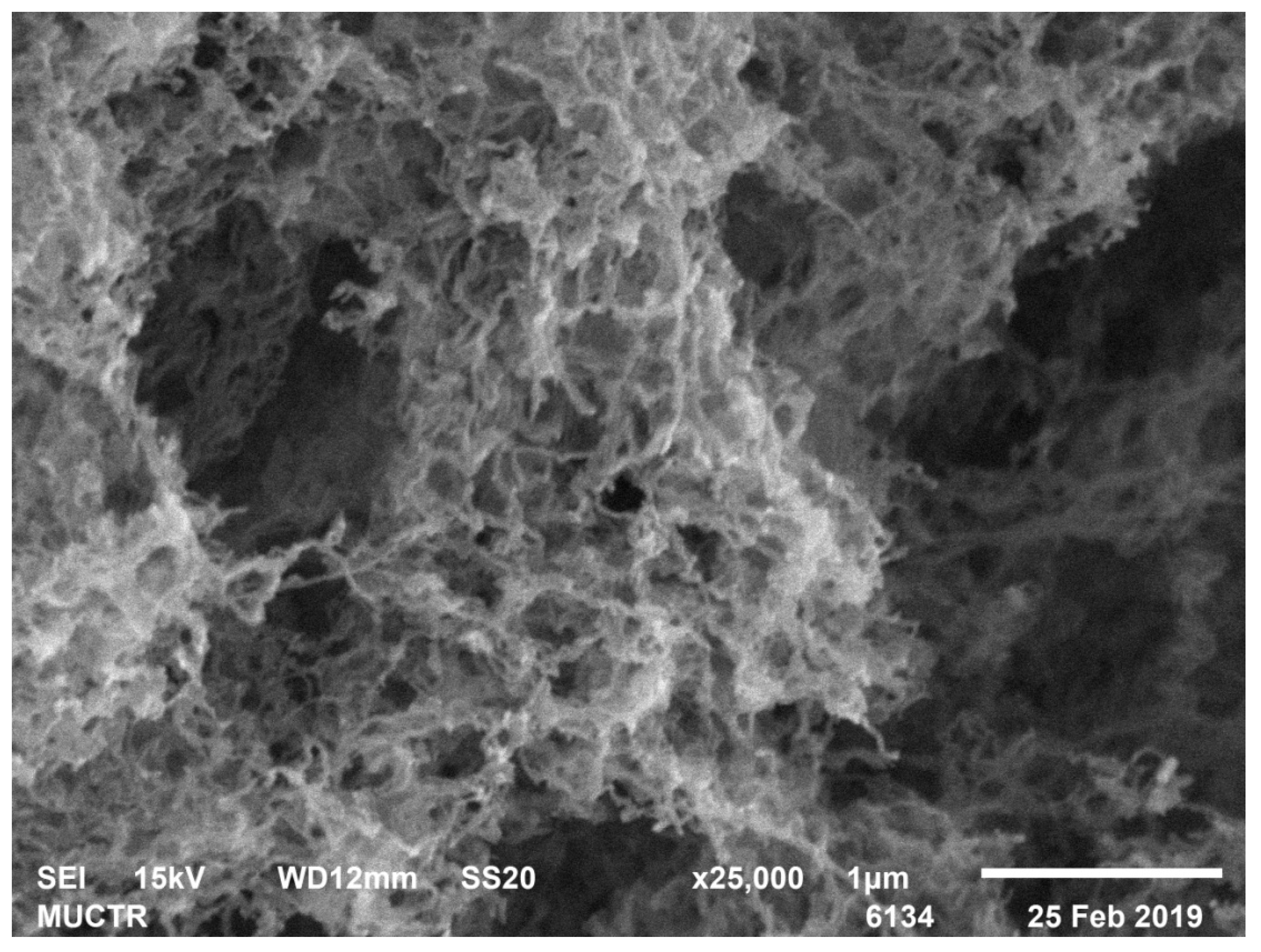
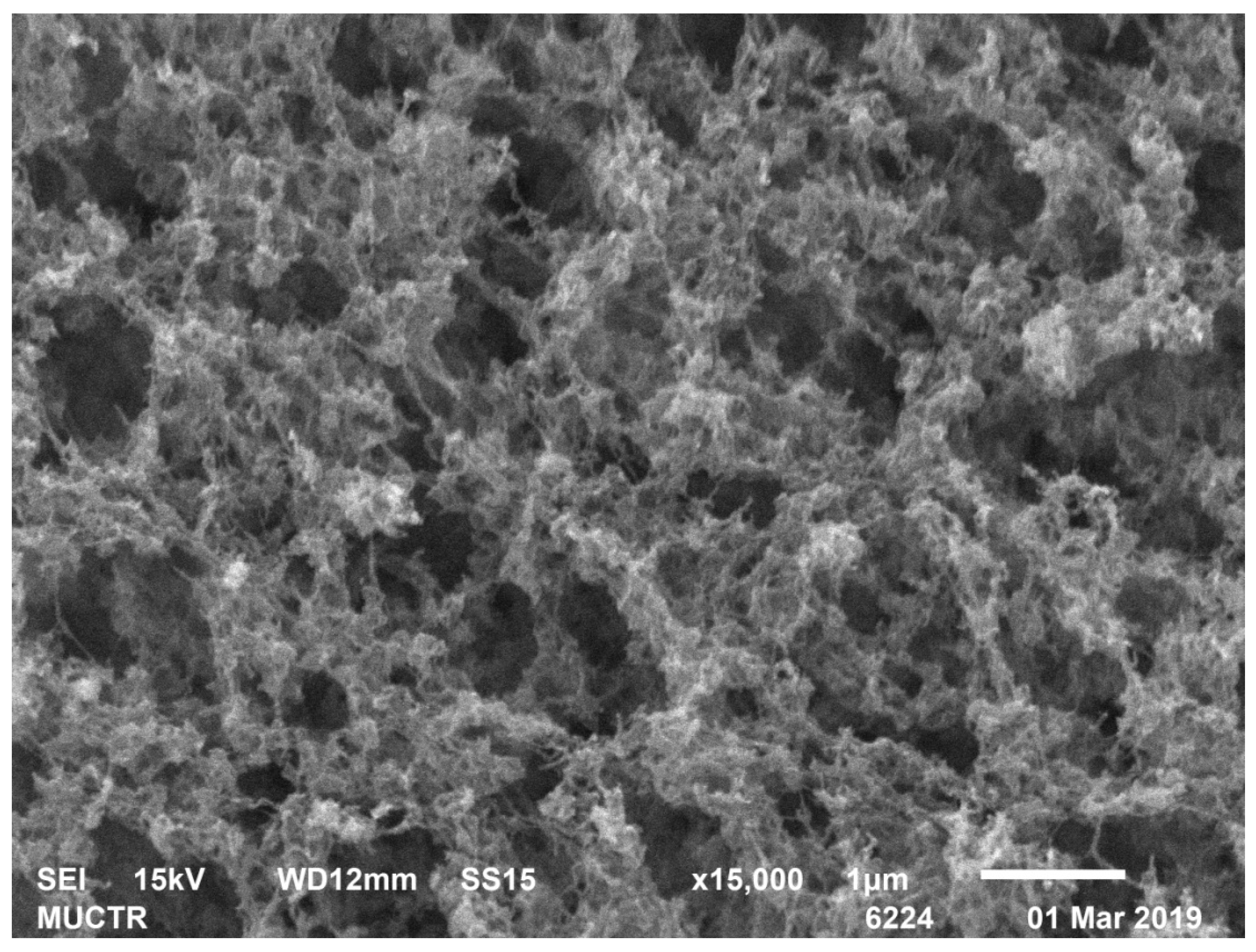
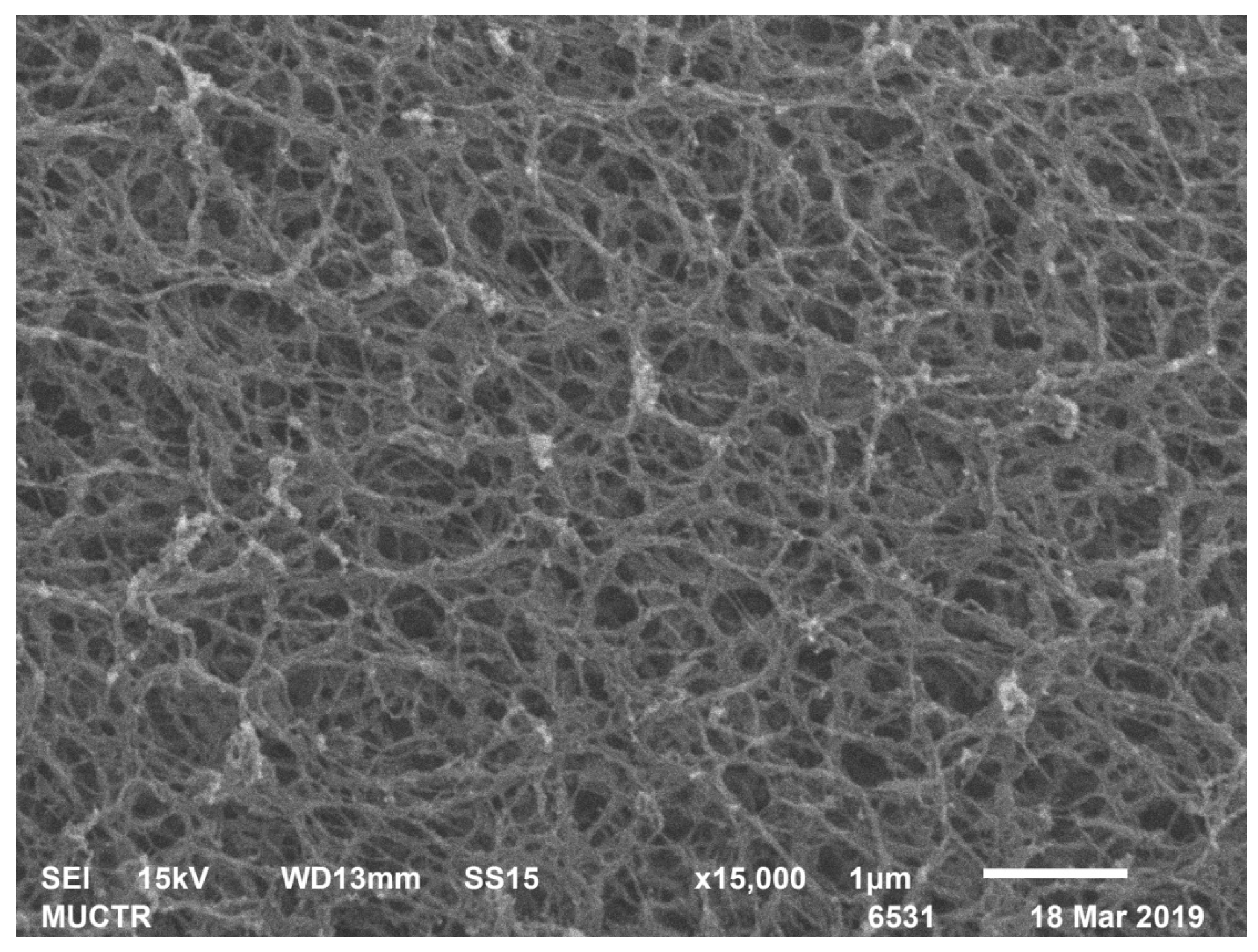
2.2. Analytical Experiments
3. Theory
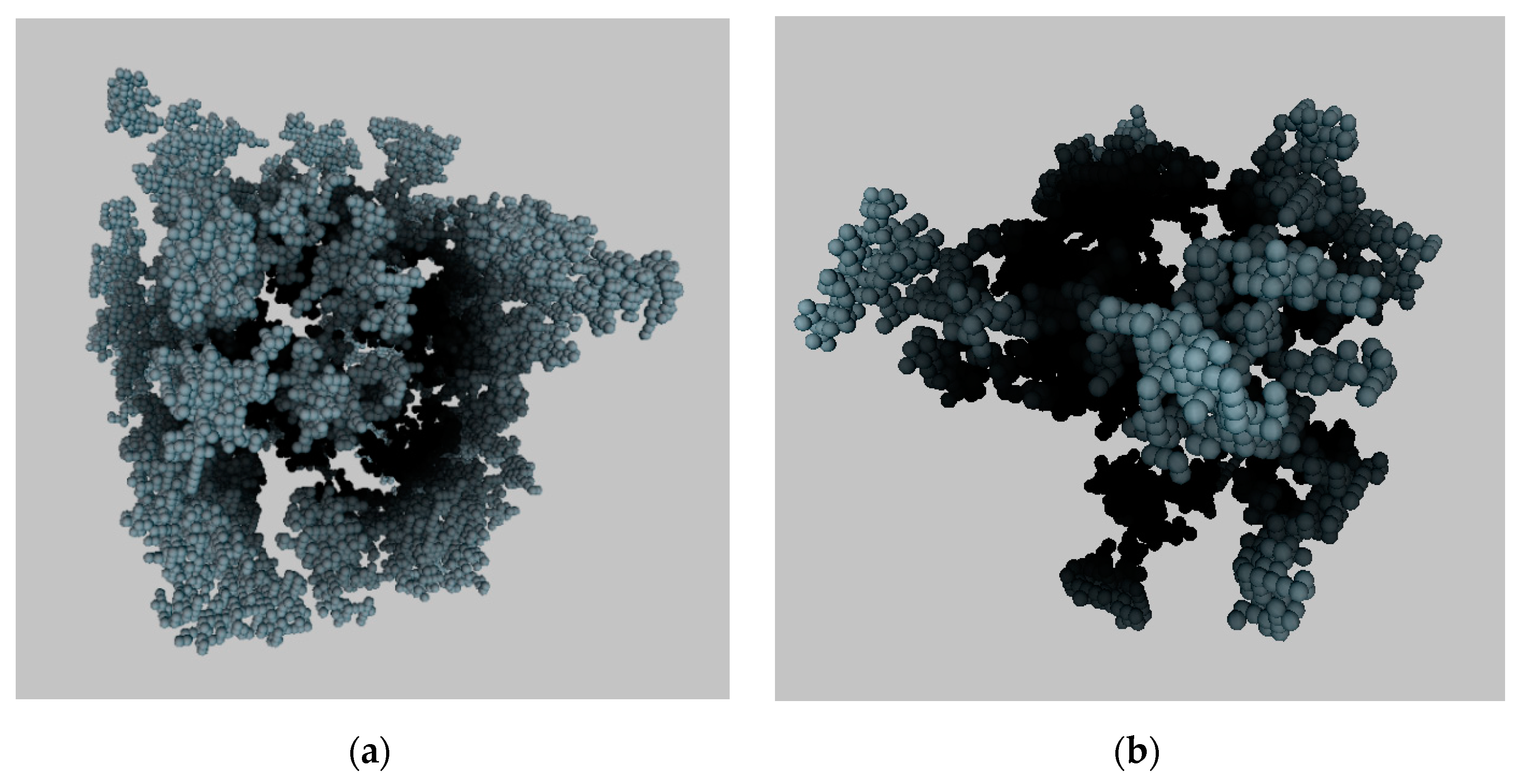
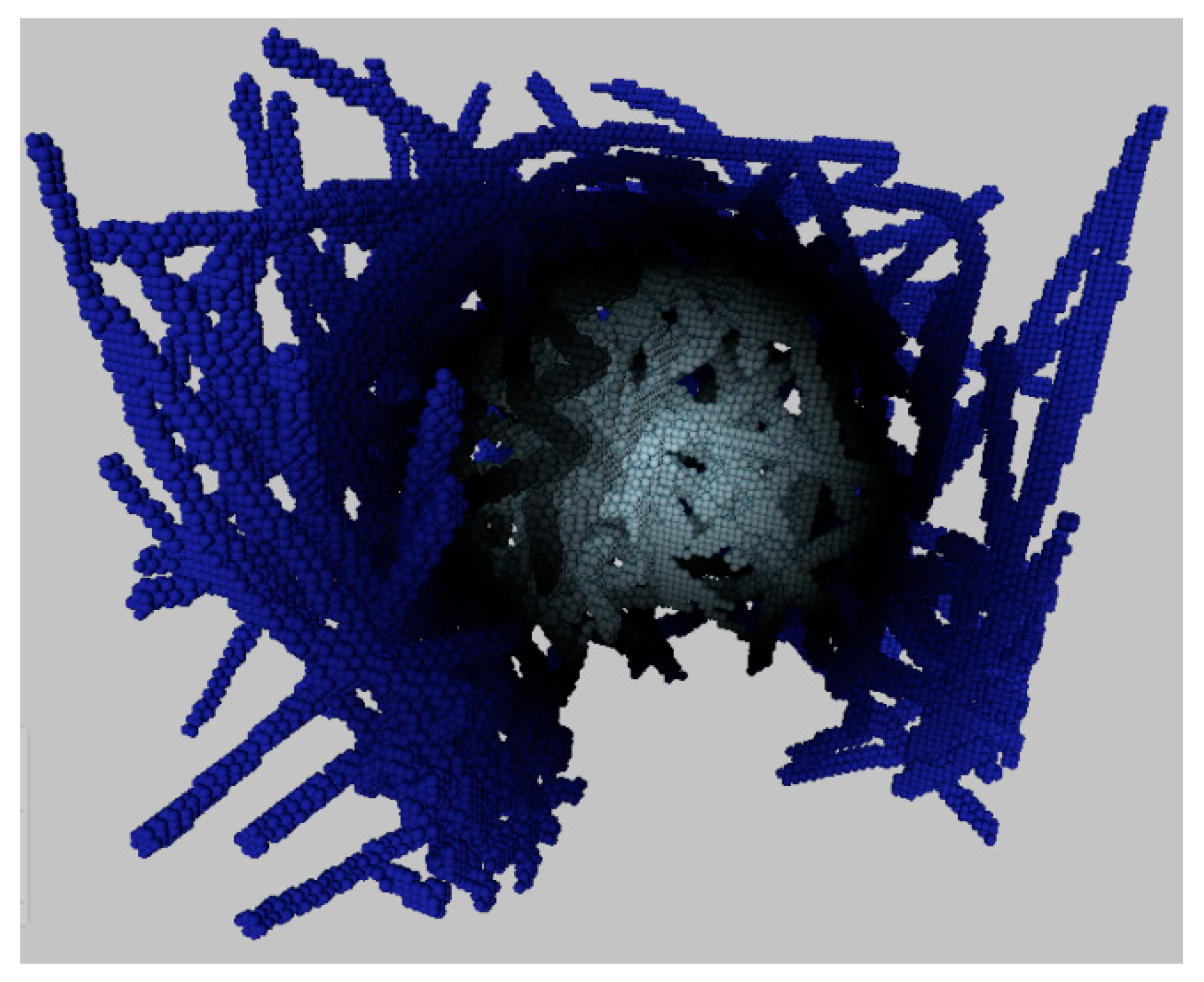
3.1. Fibrous Nanostructure Model
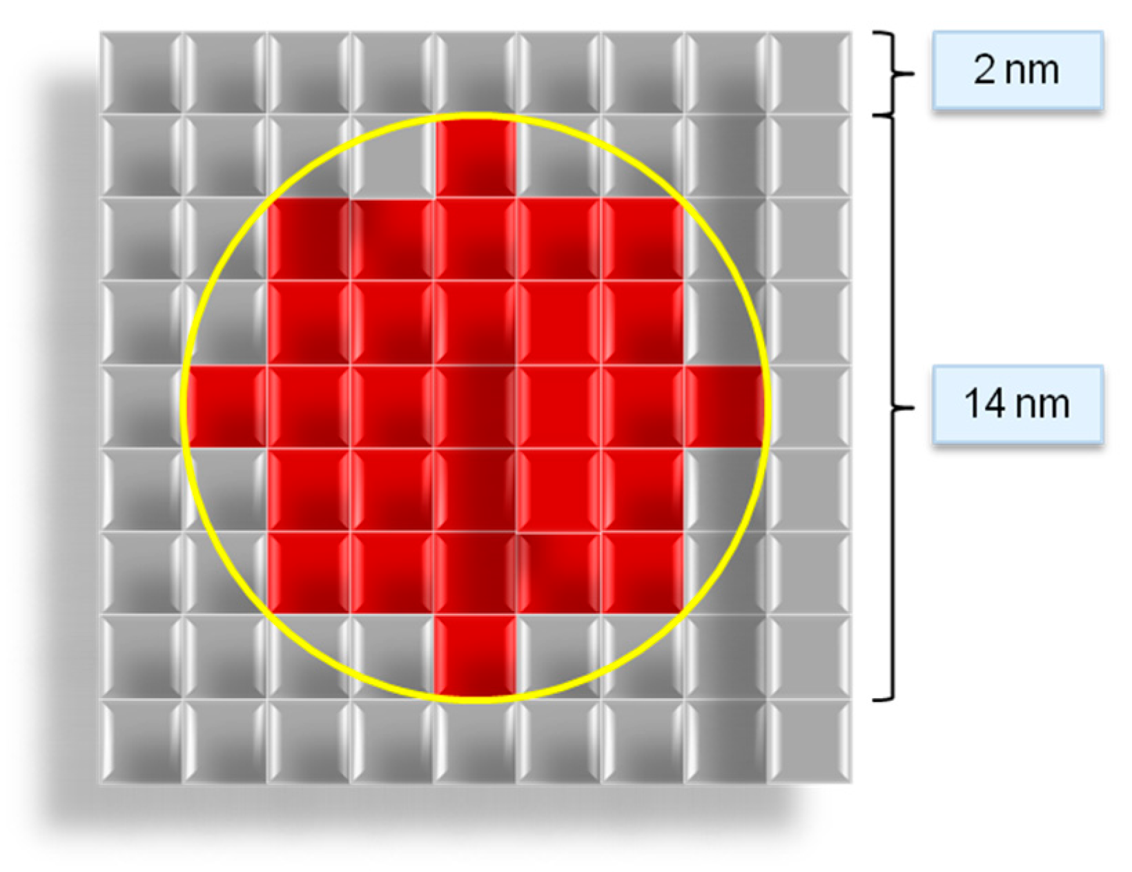
- The modeling space is divided into cells of the same size, square (two-dimensional structure) or cubic (three-dimensional structure) shapes. The scale of one cell is an integer and is specified in nanometers.
- Each cell can be in one of two given states: “fiber” and “empty”.
- Neighboring cells are cells that have a common face.
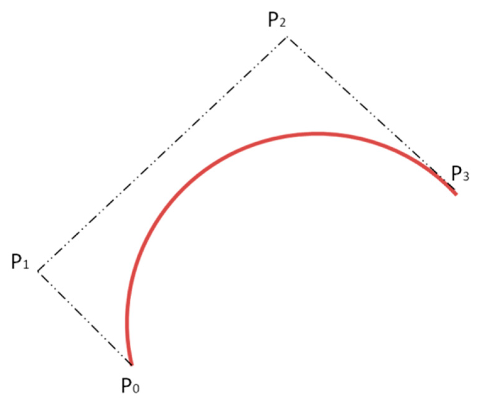
- Cells have a “fiber” state if they lie in the path of the Bezier curve.
- All fibers have the same diameter.
- The fiber diameter of the digital structure is set by a certain number of cells. Figure 11 shows an example of a fiber cross-section as a set of cells at a scale of one cell of 2 nm.
- The beginning and end of the fiber lie on the edges of the modeling space.
3.2. Digital Structure Parameters Evaluation
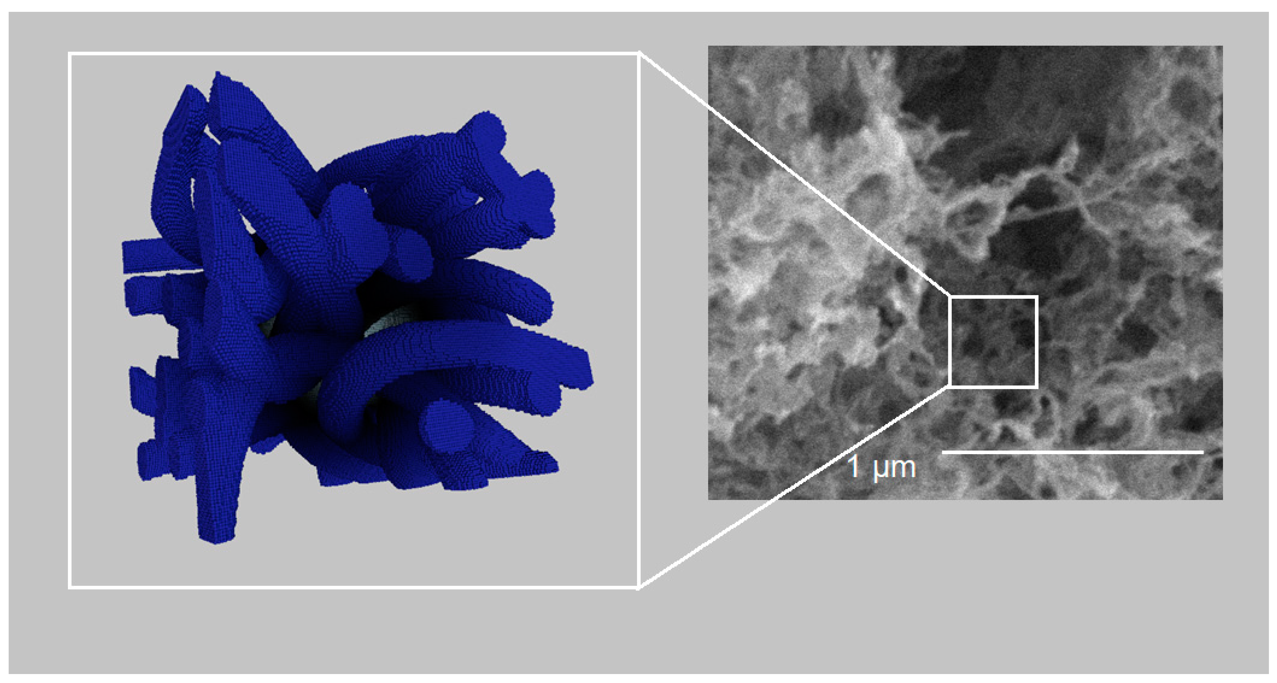
4. Results
5. Discussion
6. Conclusions
Author Contributions
Funding
Conflicts of Interest
References
- Smirnova, I.; Gurikov, P. Aerogel production: Current status, research directions, and future opportunities. J. Supercrit. Fluids 2018, 134, 228–233. [Google Scholar] [CrossRef]
- Lovskaya, D.; Lebedev, A.; Menshutina, N. Aerogels as drug delivery systems: In vitro and in vivo evaluations. J. Supercrit. Fluids 2015, 106, 115–121. [Google Scholar] [CrossRef]
- Solovieva, A.B.; Kopylov, A.S.; Savko, M.A.; Zarkhina, T.S.; Lovskaya, D.D.; Lebedev, A.E.; Menshutina, N.V.; Krivandin, A.V.; Shershnev, I.V.; Kotova, S.L.; et al. Photocatalytic Properties of Tetraphenylporphyrins Immobilized on Calcium Alginate Aerogels. Sci. Rep. 2017, 7, 12640. [Google Scholar] [CrossRef] [PubMed] [Green Version]
- Fischer, F.; Rigacci, A.; Pirard, R.; Berthon-Fabry, S.; Achard, P. Cellulose-based aerogels. Polymer 2006, 47, 7636–7645. [Google Scholar] [CrossRef]
- Jin, H.; Nishiyama, Y.; Wada, M.; Kuga, S. Nanofibrillar cellulose aerogels. Colloids Surf. A Physicochem. Eng. Asp. 2004, 240, 63–67. [Google Scholar] [CrossRef]
- Weatherwax, R.; Caulfield, D. Cellulose aerogels: An improved method for preparing a highly expanded form of dry cellulose. Tappi 1971, 54, 985–986. [Google Scholar]
- Lisuzzo, L.; Cavallaro, G.; Milioto, S.; Lazzara, G. Halloysite Nanotubes Coated by Chitosan for the Controlled Release of Khellin. Polymers 2020, 12, 1766. [Google Scholar] [CrossRef]
- Krystyjan, M.; Khachatryan, G.; Grabacka, M.; Krzan, M.; Witczak, M.; Grzyb, J.; Woszczak, L. Physicochemical, Bacteriostatic, and Biological Properties of Starch/Chitosan Polymer Composites Modified by Graphene Oxide, Designed as New Bionanomaterials. Polymers 2021, 13, 2327. [Google Scholar] [CrossRef]
- Sivanesan, I.; Gopal, J.; Muthu, M.; Shin, J.; Oh, J.-W. Reviewing Chitin/Chitosan Nanofibers and Associated Nanocomposites and Their Attained Medical Milestones. Polymers 2021, 13, 2330. [Google Scholar] [CrossRef]
- Bandman, O. 3-D Cellular Automata Model of Fluid Permeation through Porous Material. In Proceedings of the 12th International Conference on Parallel Computing Technologies, PaCT 2013, St. Petersburg, Russia, 30 September–4 October 2013; Springer: Berlin/Heidelberg, Germany, 2013; pp. 278–290. [Google Scholar] [CrossRef]
- Bandman, O. Parallelization efficiency versus stochasticity in simulation reaction–diffusion by cellular automata. J. Supercomput. 2016, 73, 687–699. [Google Scholar] [CrossRef]
- Bezbradica, M.; Crane, M.; Ruskin, H.J. Parallelisation strategies for large scale cellular automata frameworks in pharmaceu-tical modelling. In Proceedings of the 2012 International Conference on High Performance Computing & Simulation (HPCS)‒IEEE, Madrid, Spain, 2–6 July 2012; pp. 223–230. [Google Scholar]
- Brieger, L.; Bonomi, E. Cellular automata—lattice gas models for PD′’s. Comp. Phys. Commun. 1992, 73, 47–60. [Google Scholar] [CrossRef]
- Ferrando, N.; Gosalvez, M.; Cerdá, J.; Gadea, R.; Sato, K. Octree-based, GPU implementation of a continuous cellular autom-aton for the simulation of complex, evolving surfaces. Comp. Phys. Commun. 2011, 182, 628–640. [Google Scholar] [CrossRef] [Green Version]
- Hansen, P.B. Parallel cellular automata: A model program for computational science. Concurr. Pr. Exp. 1993, 5, 425–448. [Google Scholar] [CrossRef] [Green Version]
- Kolnoochenko, A.; Gurikov, P.; Menshutina, N. General-purpose graphics processing units application for diffusion simulation using cellular automata. Comp. Aid. Chem. Eng. 2011, 29, 166–170. [Google Scholar] [CrossRef]
- Rybacki, S.; Himmelspach, J.; Uhrmacher, A.M. Experiments with single core, multi-core, and GPU based computation of cellular automata. In Proceedings of the First International Conference on Advances in System Simulation, IEEE, Porto, Portugal, 20–25 September 2009; pp. 62–67. [Google Scholar]
- Sander, L.M. Diffusion-limited aggregation: A kinetic critical phenomenon? Contemp. Phys. 2000, 41, 203–218. [Google Scholar] [CrossRef]
- Finegold, L. Cell membrane fluidity: Molecular modeling of particle aggregations seen in electron microscopy. Biochim. Biophys. Acta Biomembr. 1976, 448, 393–398. [Google Scholar] [CrossRef]
- Meakin, P. Formation of Fractal Clusters and Networks by Irreversible Diffusion-Limited Aggregation. Phys. Rev. Lett. 1983, 51, 1119–1122. [Google Scholar] [CrossRef]
- Fry, D.; Mohammad, A.; Chakrabarti, A.; Sorensen, C.M. Cluster Shape Anisotropy in Irreversibly Aggregating Particulate Systems. Langmuir 2004, 20, 7871–7879. [Google Scholar] [CrossRef]
- Meakin, P. A Historical Introduction to Computer Models for Fractal Aggregates. J. Sol. Gel Sci. Technol. 1999, 15, 97–117. [Google Scholar] [CrossRef]
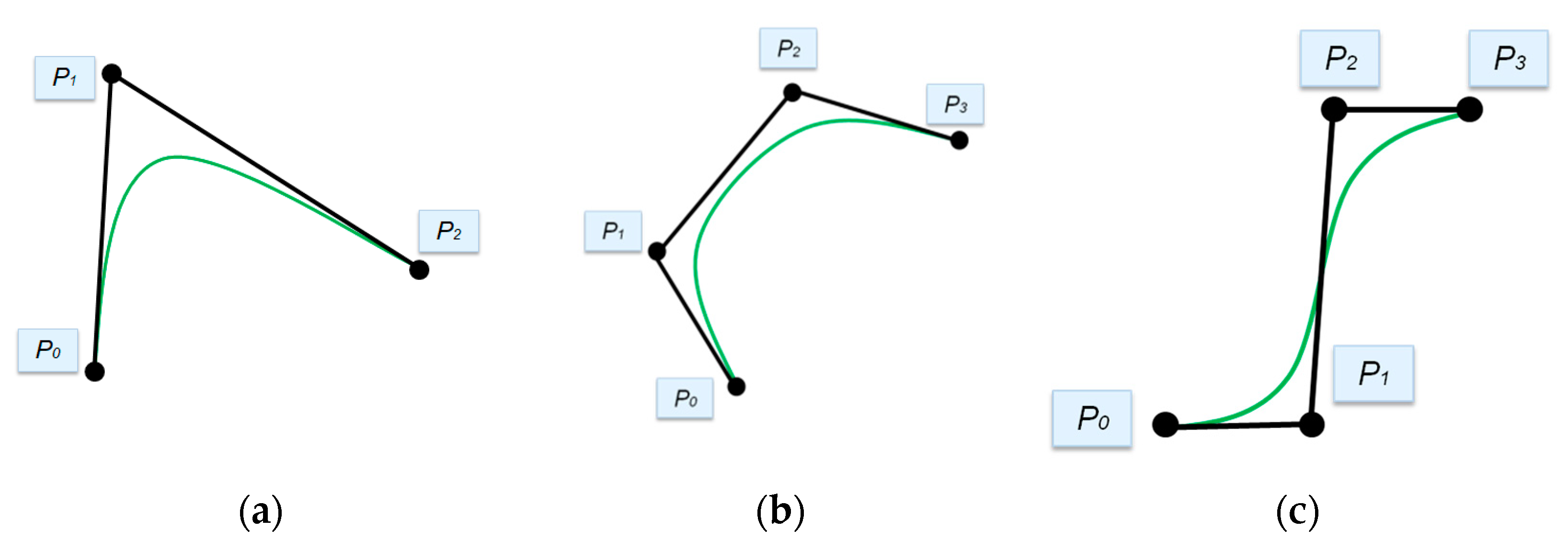
- Civicioglu, P.; Besdok, E. Bezier Search Differential Evolution Algorithm for numerical function optimization: A comparative study with CRMLSP, MVO, WA, SHADE and LSHADE. Expert Syst. Appl. 2021, 165, 113875. [Google Scholar] [CrossRef]
- Forrest, A.R. Interactive Interpolation and Approximation by Bezier Polynomials. Comput. J. 1972, 15, 71–79. [Google Scholar] [CrossRef]
- Faigl, J.; Váňa, P. Surveillance planning with Bézier curves. IEEE Robot. Auto. Lett. 2018, 3, 750–757. [Google Scholar] [CrossRef]
- Elhoseny, M.; Shehab, A.; Yuan, X. Optimizing robot path in dynamic environments using Genetic Algorithm and Bezier Curve. J. Intell. Fuzzy Syst. 2017, 33, 2305–2316. [Google Scholar] [CrossRef] [Green Version]
- Chu, C.-H.; Séquin, C.H. Developable Bézier patches: Properties and design. Comput. Des. 2002, 34, 511–527. [Google Scholar] [CrossRef]
- Lovskaya, D.; Menshutina, N.; Mochalova, M.; Nosov, A.; Grebenyuk, A. Chitosan-Based Aerogel Particles as Highly Effective Local Hemostatic Agents. Production Process and In Vivo Evaluations. Polymers 2020, 12, 2055. [Google Scholar] [CrossRef] [PubMed]
- Lovskaya, D.; Menshutina, N. Alginate-Based Aerogel Particles as Drug Delivery Systems: Investigation of the Supercritical Adsorption and In Vitro Evaluations. Materials 2020, 13, 329. [Google Scholar] [CrossRef] [Green Version]
- Menshutina, N.; Lovskaya, D.; Lebedev, A.; Lebedev, E. Production of sodium alginate-based aerogel particles using super-critical drying in units with different volumes. Rus. J. Phys. Chem. B 2017, 11, 1296–1305. [Google Scholar] [CrossRef]
- Menshutina, N.; Lebedev, I.; Lebedev, E.; Paraskevopoulou, P.; Chriti, D.; Mitrofanov, I. A Cellular Automata Approach for the Modeling of a Polyamide and Carbon Aerogel Structure and Its Properties. Gels 2020, 6, 35. [Google Scholar] [CrossRef]


 —“fiber” cells,
  —“empty” cells, ⚫—control points,
  —Bezier curves.
—“fiber” cells, —“empty” cells, ⚫—control points, —Bezier curves.
—Bezier curves.
—“fiber” cells, —“empty” cells, ⚫—control points, —Bezier curves.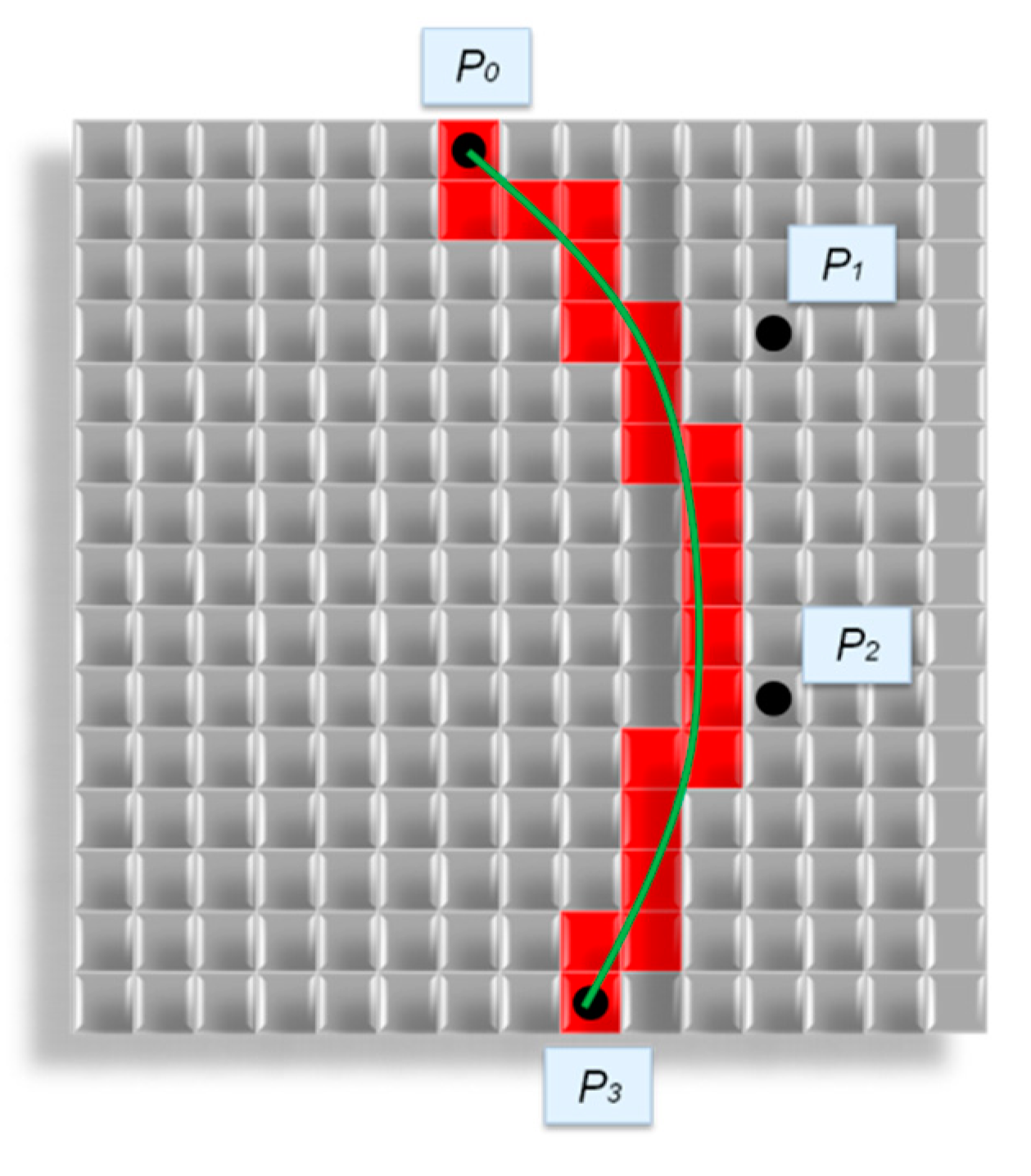 —“fiber” cells,
  —“fiber” cells, added after diameter increase, —“empty” cells, —circles, formed around “fiber” cells: (a) Forming circles around “fiber” cells; (b) Changing states of cells inside circles into “fiber”.
—“fiber” cells, —“fiber” cells, added after diameter increase, —“empty” cells, —circles, formed around “fiber” cells: (a) Forming circles around “fiber” cells; (b) Changing states of cells inside circles into “fiber”.
—“fiber” cells, added after diameter increase, —“empty” cells, —circles, formed around “fiber” cells: (a) Forming circles around “fiber” cells; (b) Changing states of cells inside circles into “fiber”.
—“fiber” cells, —“fiber” cells, added after diameter increase, —“empty” cells, —circles, formed around “fiber” cells: (a) Forming circles around “fiber” cells; (b) Changing states of cells inside circles into “fiber”.


| Sample № | Cchitosan, Mass% | Cacid, M | Calkali, M | Cpolymer, Mass% |
|---|---|---|---|---|
| 1 | 1 | 0.1 | 1 | 0 |
| 2 | 1 | 0.2 | 1 | 0 |
| 3 | 2 | 0.1 | 1 | 0 |
| 4 | 2 | 0.2 | 1 | 0 |
| 5 | 1 | 0.1 | 1 | 0.05 |
| 6 | 1 | 0.2 | 1 | 0.05 |
| 7 | 2 | 0.1 | 1 | 0.05 |
| 8 | 2 | 0.2 | 1 | 0.05 |
| 9 | 1 | 0.1 | 0.1 | 0 |
| 10 | 1 | 0.2 | 0.1 | 0 |
| 11 | 2 | 0.1 | 0.1 | 0 |
| 12 | 2 | 0.2 | 0.1 | 0 |
| 13 | 1 | 0.1 | 0.1 | 0.05 |
| 14 | 1 | 0.2 | 0.1 | 0.05 |
| 15 | 2 | 0.1 | 0.1 | 0.05 |
| 16 | 2 | 0.2 | 0.1 | 0.05 |
| Sample № | SBET, m2/g | Vpore, cm3/g | ρskeletal, kg/m3 | ρbulk, kg/m3 | Porosity, % |
|---|---|---|---|---|---|
| 1 | 301 ± 2.13 | 1.28 | 2050 | 55 | 98.27 |
| 2 | 270 ± 2.11 | 1.32 | 1909 | 48 | 97.44 |
| 3 | 166 ± 1.99 | 0.74 | 1893 | 66 | 96.49 |
| 4 | 192 ± 2.12 | 1.07 | 1842 | 86 | 95.30 |
| 5 | 151 ± 2.15 | 0.07 | 1880 | 34 | 98.16 |
| 6 | 360 ± 2.15 | 1.80 | 2367 | 38 | 98.35 |
| 7 | 143 ± 1.87 | 0.79 | 2129 | 67 | 96.84 |
| 8 | 237 ± 2.17 | 1.43 | 1741 | 62 | 96.40 |
| 9 | 261 ± 2.16 | 1.50 | 1743 | 52 | 97.01 |
| 10 | 323 ± 1.96 | 2.25 | 1788 | 53 | 96.99 |
| 11 | 347 ± 2.01 | 2.26 | 1676 | 64 | 98.13 |
| 12 | 135 ± 2.06 | 0.93 | 2232 | 52 | 97.63 |
| 13 | 248 ± 1.98 | 1.72 | 1933 | 49 | 97.44 |
| 14 | 227 ± 2.03 | 1.39 | 3307 | 39 | 98.80 |
| 15 | 190 ± 2.11 | 1.28 | 1778 | 54 | 96.93 |
| 16 | 175 ± 2.07 | 1.10 | 2247 | 49 | 97.81 |
| Sample № | Fiber Diameter, nm | Porositynit, % | SBET exp., m2/g | SBET dig., m2/g | Deviation, % |
|---|---|---|---|---|---|
| 1 | 30 | 67 | 301 | 293 | 3 |
| 2 | 34 | 68 | 270 | 280 | 4 |
| 3 | 42 | 55 | 166 | 161 | 3 |
| 4 | 46 | 64 | 192 | 176 | 8 |
| 5 | 42 | 54 | 151 | 168 | 11 |
| 6 | 30 | 74 | 360 | 343 | 5 |
| 7 | 34 | 53 | 143 | 137 | 4 |
| 8 | 30 | 77 | 237 | 229 | 3 |
| 9 | 30 | 65 | 261 | 258 | 1 |
| 10 | 34 | 64 | 323 | 317 | 2 |
| 11 | 34 | 72 | 347 | 340 | 2 |
| 12 | 42 | 66 | 135 | 128 | 5 |
| 13 | 26 | 67 | 248 | 256 | 3 |
| 14 | 34 | 73 | 227 | 213 | 6 |
| 15 | 34 | 58 | 190 | 187 | 1 |
| 16 | 38 | 67 | 175 | 191 | 9 |
Publisher’s Note: MDPI stays neutral with regard to jurisdictional claims in published maps and institutional affiliations. |
© 2021 by the authors. Licensee MDPI, Basel, Switzerland. This article is an open access article distributed under the terms and conditions of the Creative Commons Attribution (CC BY) license (https://creativecommons.org/licenses/by/4.0/).
Share and Cite
Lebedev, I.; Lovskaya, D.; Mochalova, M.; Mitrofanov, I.; Menshutina, N. Cellular Automata Modeling of Three-Dimensional Chitosan-Based Aerogels Fiberous Structures with Bezier Curves. Polymers 2021, 13, 2511. https://doi.org/10.3390/polym13152511
Lebedev I, Lovskaya D, Mochalova M, Mitrofanov I, Menshutina N. Cellular Automata Modeling of Three-Dimensional Chitosan-Based Aerogels Fiberous Structures with Bezier Curves. Polymers. 2021; 13(15):2511. https://doi.org/10.3390/polym13152511
Chicago/Turabian StyleLebedev, Igor, Daria Lovskaya, Maria Mochalova, Igor Mitrofanov, and Natalia Menshutina. 2021. "Cellular Automata Modeling of Three-Dimensional Chitosan-Based Aerogels Fiberous Structures with Bezier Curves" Polymers 13, no. 15: 2511. https://doi.org/10.3390/polym13152511
APA StyleLebedev, I., Lovskaya, D., Mochalova, M., Mitrofanov, I., & Menshutina, N. (2021). Cellular Automata Modeling of Three-Dimensional Chitosan-Based Aerogels Fiberous Structures with Bezier Curves. Polymers, 13(15), 2511. https://doi.org/10.3390/polym13152511