A Note for Probabilistic Model of Polymer Crystallization in Temperature Gradients

Abstract

A polymer crystallization kinetics model is the most important way to characterize the crystallization rate of polymers. Because polymers are poor heat conductors, the cooling of thick-walled shapes results in temperature gradients. Piorkowska (Piorkowska, E. J. Appl. Polym. Sci., 2002, 86: 1351–1362.) derived the probabilistic analytical model of polymer crystallization in temperature gradients based on the Avrami equation. However, there are some misunderstandings when using this model. Here, isotactic polypropylene (iPP) is chosen as a model polymer and its crystallization is studied in a temperature gradient field. Based on the results of the Monte Carlo method, the probabilistic model methodology is discussed. The results show that when the product has a large temperature gradient and a large temperature difference, the probabilistic model cannot be used directly; instead, it is necessary to use the average probabilistic model. This means that the sample should be divided into several smaller parts and the probabilistic model used separately for each small part. The values are then averaged to obtain the mean conversion degree of the melt into spherulites for the whole product. The effects of the division number are also discussed. The goal of the present paper is to better understand the polymer crystallization kinetics model in terms of temperature gradients.

1. Introduction

In the past few decades, polymers have played an important role in industry because of their excellent properties [1,2]. Many polymers have the ability to crystallize. For crystalline polymers, the crystallization behavior is the key factor affecting their microstructure and determining the final properties of the polymer products [2]. During polymer processing, crystallization mainly occurs during the cooling stage. Polymers are poor heat conductors, and thus the cooling of thick-walled shapes results in temperature gradients [3,4]. Moreover, the latent heat generated by crystallization causes an increase in temperature, which aggravates the temperature gradient. Therefore, it is of great significance to study polymer crystallization in terms of temperature gradients.

The polymer crystallization kinetics model is an important way to characterize the crystallization rate of polymers. Piorkowska derived the probabilistic analytical model of polymer crystallization in temperature gradients based on the Avrami equation [5,6]. Piorkowska found that in the numerical simulation of isotactic polypropylene (iPP) under a uniaxial temperature gradient, the probabilistic analytical model did a good job of predicting the conversion degree compared with the experimental results in the case of low nucleation density with the central temperature set as $T_0>125$ °C. However, in our previous study [7,8], we found that the conversion degree predicted by the probabilistic model was far from that obtained by the Monte Carlo results at low central temperatures ($T_0\le 125$ °C) and high temperature gradients. Therefore, there are some misunderstandings when using the probabilistic model. A thorough investigation of this model should be conducted.

The crystallization kinetics model is very important in polymer crystallization studies not only on the mesoscopic scale for isothermal or nonisothermal cases but also in multi-scale studies in conjunction with energy equations [2,9,10,11,12,13,14,15]. Therefore, this paper takes iPP as the model polymer and discusses the way of using the probabilistic model under temperature gradients based on our previous work.

The objective of this paper is to discuss the methodology of the probabilistic model proposed by Piorkowska [5]. The structure of this paper is as follows: In Section 2, we mainly introduce the probabilistic model, the nucleation and growth model of iPP, and the Monte Carlo method; in Section 3, we present the poor results that occur when using the probabilistic model directly, the methods used to overcome these problems, and the effects of the division number; in Section 4, we give the conclusion of the paper.

2. Mathematical Model and Numerical Method

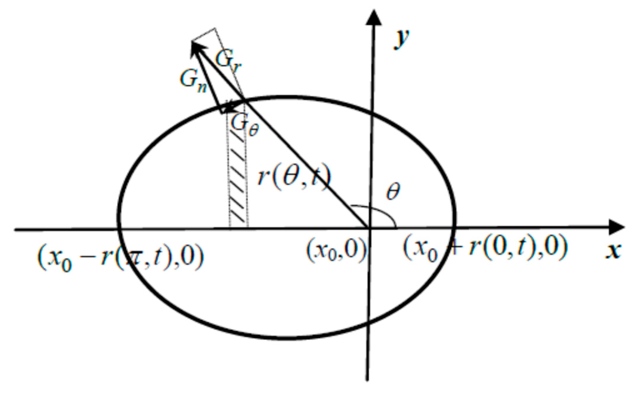
2.1. Probabilistic Model

Piorkowska derived the probabilistic analytical model of polymer crystallization in temperature gradients based on the Avrami equation [5]. The method was based on the “extended volume” method, which did not consider the impingement between grains and considered the growth space to be infinite and unrestricted.

For the two-dimensional case, considering the growth morphology shown in Figure 1, the polymer tends to form anisotropic spherulites in a temperature gradient. The “extended volume” of a single crystal is

$$V(x_0,t)=2{\int }_{x_0-r(\pi ,t)}^{x_0+r(0,t)}|x-x_0||\tan \theta |dx$$

(1)

Here,

$$|\tan \theta |=\sqrt{\frac{1}{{\cos }^2\theta }-1}$$

(2)

From Figure 1, we know that

$$\{\begin{array}{l}dx/dr=\cos \theta \\ dr=G_{r}dt\end{array}$$

(3)

Here, $G_r$ is the radial growth rate of the crystal. By integration, we obtain

$$t={\cos }^{-1}\theta {\displaystyle \underset{x_0}{\overset{x}{\int }}{G}_r{(x^{\prime })}^{-1}}d{x}^{\prime }$$

(4)

where t is the crystallization time. Equation (4) is equivalent to

$$\cos \theta ={\displaystyle \underset{x_0}{\overset{x}{\int }}{G}_r{(x^{\prime })}^{-1}}d{x}^{\prime }/t$$

(5)

Therefore, the “extended volume” of a single crystal is

$$V(x_0,t)=2{\int }_{x_0-r(\pi ,t)}^{x_0+r(0,t)}|x-x_0|{\left\{t^2{\left[{\int }_{x_0}^x{G}_r^{-1}(x^{\prime })d{x}^{\prime }\right]}^{-2}-1\right\}}^{1/2}dx$$

(6)

Because the system has a nucleation density of $D$, the “extended volume” of all crystals is [5]

$$E(x_0,t)=2{\int }_{x_0-r(\pi ,t)}^{x_0+r(0,t)}D|x-x_0|{\left\{t^2{\left[{\int }_{x_0}^x{G}_r^{-1}(x^{\prime })d{x}^{\prime }\right]}^{-2}-1\right\}}^{1/2}dx$$

(7)

The relationship between the “extended volume” and the conversion degree satisfies the Avrami equation, which is [6]

$$\alpha =1-\exp \left[-E(x_0,t)\right]$$

(8)

where $\alpha$ is the conversion degree of the crystals.

Equations (7) and (8) are the probabilistic model proposed by Piorkowska [5]. The reason for calling probabilistic model is probably because the result is deduced by the probability of amorphous phase ($1-\alpha$) which no crystallization occurs in the volume except the extended volume. This model did a good job of predicting the conversion degree compared with the experimental results [7] in a uniaxial temperature gradient with the central temperature set as $T_0>125$ °C.

2.2. Nucleation and Growth Model of iPP

Here, we take iPP as a model polymer and discuss the crystallization kinetics model in temperature gradients. We assume that the temperature gradient is in the x direction and the temperature T obeys a linear distribution, namely, $T=T_0+\mathsf{\Lambda }\cdot x$, where $T_0$ is the central temperature and $\mathsf{\Lambda }$ is the temperature gradient [5]. The nucleation and growth model given here are fitted by the experiment results, which are [5,16]

$$D=\exp [111.265-0.2544(T+273.15)]/{\mathrm{mm}}^3$$

(9)

$$G_n=G_0\exp \left\{-U^{*}/\left[R_g(T-T_{\infty })\right]\right\}\exp \left\{-K_g/\left[T(T_m^0-T)\right]\right\}$$

(10)

Here, $D$ is the nucleation density and $G_n$ is the normal growth rate. The parameters in Equation (10) are: $U^{*}$ is an energy parameter similar to an apparent activation energy of motion, $R_g$ is the gas constant, $T_{\infty }=T_g-30$ is considered the temperature at which no further molecular displacement is possible ($T_g$ is the glass transition temperature), and $G_0$ and $K_g$ are experimentally determined constants. For a given iPP, the parameters are as follows: $U^{*}=6279 \mathrm{J}/\mathrm{mol}$, $R_g=8.314472$, $T_{\infty }=231.2 \mathrm{K}$, $T_m^0=458.2 \mathrm{K}$. $K_g$ and $G_0$ depend on the regime of crystallization: $K_g=1.47\times {10}^5 {\mathrm{K}}^2,$ $G_0=0.3359 \mathrm{cm}/\mathrm{s}$, ($T\ge 136$ °C); $K_g=3.3\times {10}^5 {\mathrm{K}}^2,G_0=3249 \mathrm{cm}/\mathrm{s}$, ($T\le 136$ °C) [5,7].

As shown in Figure 1, the relation between the normal growth rate, $G_n$, and the radial growth rate, $G_r$, is given as follows [17,18]:

$$G_r=G_n\sqrt{1+{\left(\frac{r^{\prime }}{r}\right)}^2}$$

(11)

with $r^{\prime }=dr/d\theta$.

2.3. Monte Carlo Method

The Monte Carlo method we use here is consistent with our previous paper [8]. Here, we briefly introduce this method. Crystallization follows the steps of nucleation and growth.

At the beginning, the sample is assumed to be melt and is divided into equally sized cells with the total cell number $N_{tot}$. At $t=0 \mathrm{s}$, the nucleation is randomly generated according to the nucleation density formula. Each nucleus is distinguished by a color. For each time step $\Delta t$, the radius of each crystals is calculated and several random numbers $N_{rand}$ are generated to see if it is covered by a crystal and given the same color. This cycle lasts until $t=t_{end}$.

It should be noted that in calculating the conversion degree of the crystals, we use the following spherulite occupancy ratio:

$$\alpha =N_s/N_{tot}$$

(12)

Here, $N_s$ is the number of cells that are occupied by spherulites. The conversion degree of the crystals is related to the position of nuclei and the growth of spherulites. Therefore, this value is a random one. The random error can be overcome by averaging the multiple numerical experimental data. In this paper, since the nucleation number is large, the random error is relatively small. Therefore, the results given in this paper are the results of one numerical test.

The method of mesh generation and implementation of Monte Carlo method are not described here. We refer our previous work [8,19,20] for more details. The validity of our Monte Carlo method is proven in our previous work by the comparison of the experimental result taken by Pawlak and Piorkowska and the numerical work taken by Ouyang et al. [3,7,8].

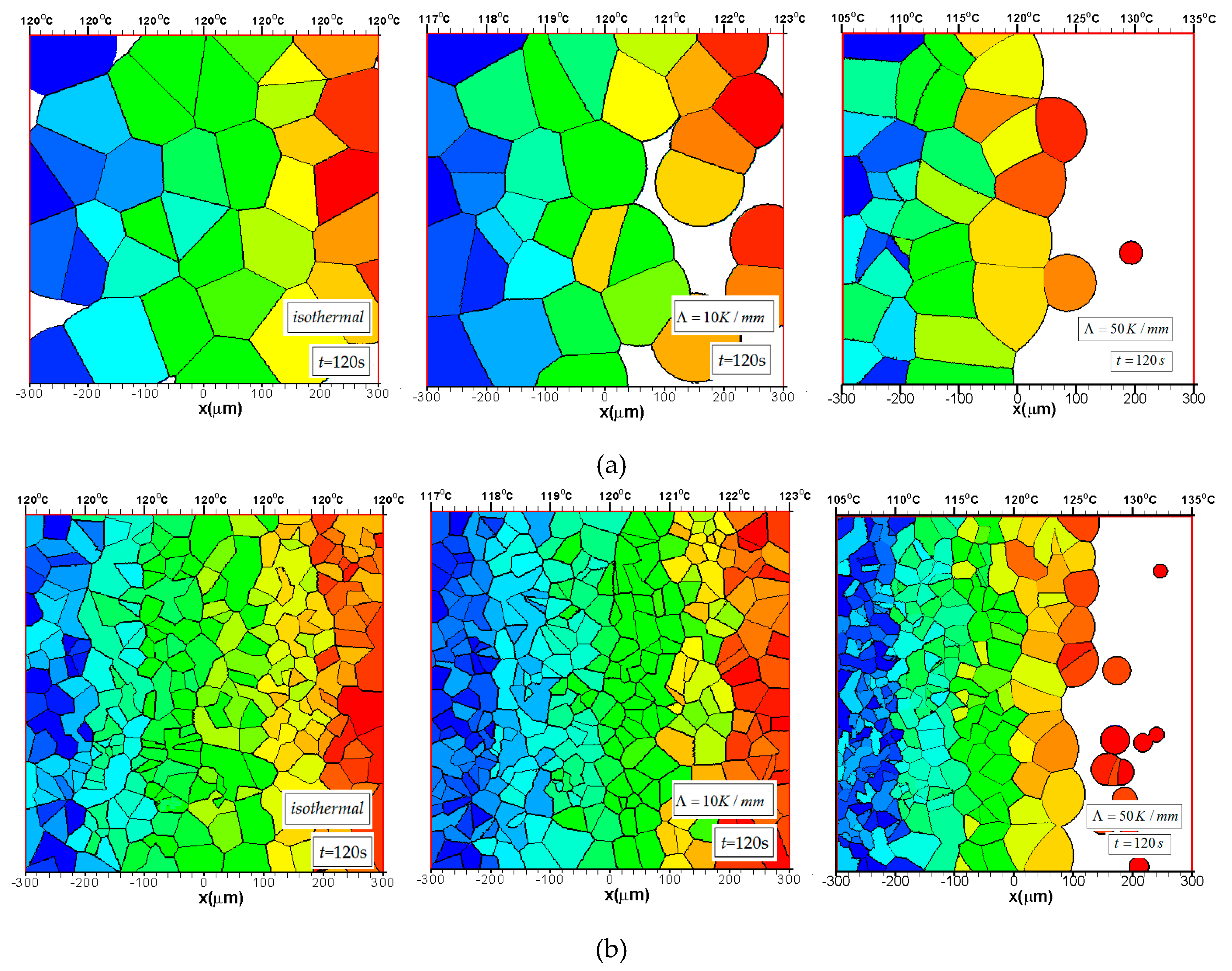
3. Results and Discussion

In this section, we first examine the performance of the probabilistic model when used directly in three nucleation density distributions: uniform distribution, a linear relationship with the normal growth rate case, and an exponential relationship between temperatures case. Then, we give a way to overcome the problem and the correct way to use the probabilistic model. Finally, we discuss the effects of the division number and the proper value of this number in the simulation.

The dimensions of the iPP sample are 600 μm × 600 μm × 11 μm. We treat the sample as two-dimension because it is very thin. The parameters used in our simulation are set as follows: total number of cells $N_{tot}=400\times 400$, total random points $N_{rand}=\mathrm{800,000}$, time step size $\Delta t=0.5$ s, divisional number in $\theta$ direction $M=100$, and initial radius of the spherulites $r^0=0$ at $t=0$ s.

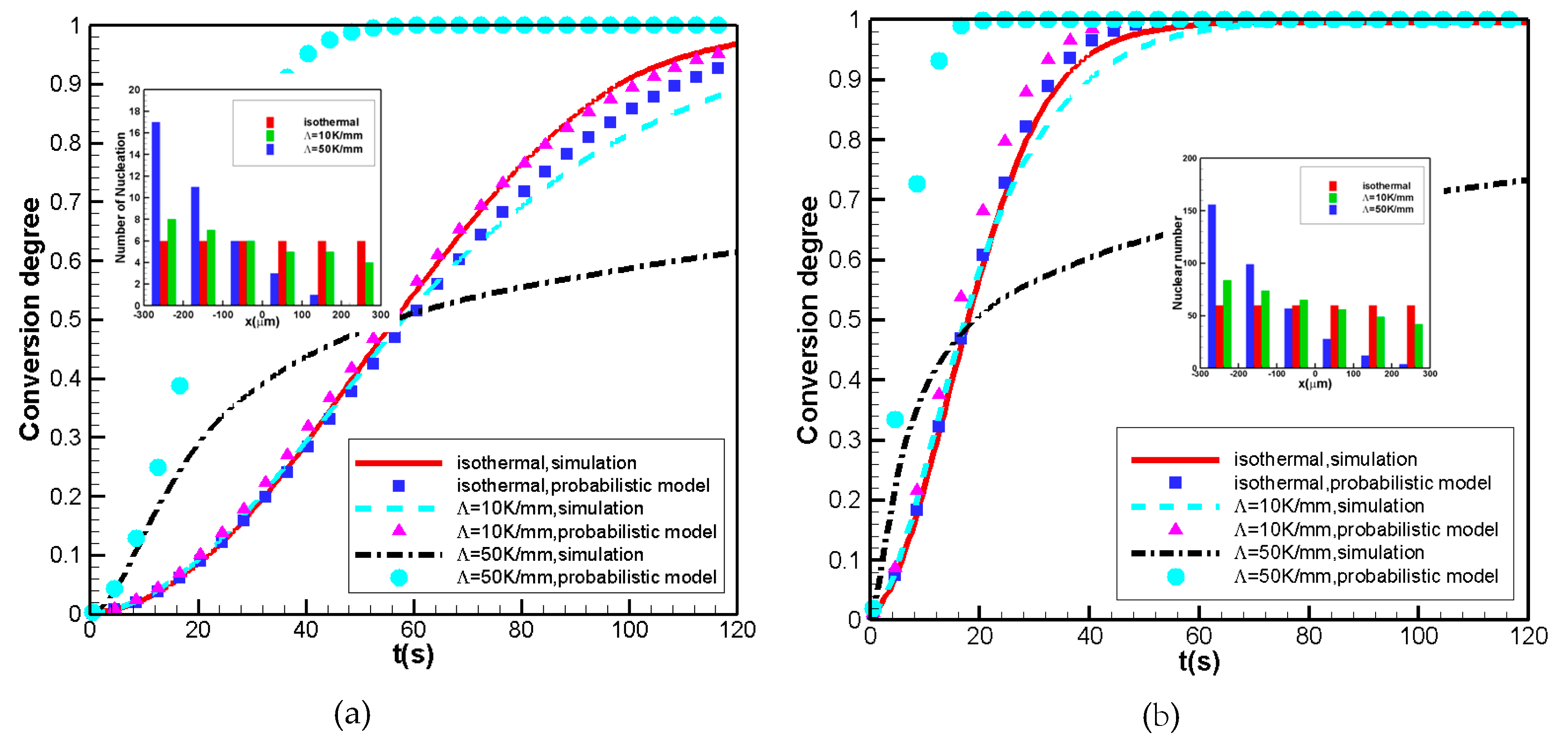
3.1. Performance of Probabilistic Model When Used Directly

3.1.1. Nucleation Density Obeys Uniform Distribution

Here, we assume the nucleation density is uniformly distributed. The nucleus center is random in the whole part, regardless of the temperature gradient. This nucleation is ideal because in most polymers, nucleation is temperature-dependent. The reason is that the probabilistic model is based on the Avrami equation while the latter required the nuclei distributed randomly in the sample. Figure 2 shows the crystal morphology predicted by the Monte Carlo method with a central temperature $T_0=120$ °C and nucleation densities of $D=100/{\mathrm{mm}}^2$ and $D=1000/{\mathrm{mm}}^2$. In our method, different spherulites are distinguished by different colors. The white background represents the melt. For the isothermal case in Figure 2a, we add a color legend to see the color assignment. We label the nucleus roughly from left to right, thus it appears that the color is related to the direction. However, the color values have no meaning, just to distinguish different crystals. It is clear that the higher temperature gradient leads to a colder temperature on the left side and a higher temperature on the right side. However, the higher temperature on the right side is not suitable for crystallization, thus leading to a decrease in the overall crystallization rate.

Figure 3 shows the comparison of the conversion degree of the melt into spherulites between the Monte Carlo method and the probabilistic model at different nucleation densities. According to Figure 3, the results of the probabilstic model agree well with the Monte Carlo results for the isothermal $(\mathsf{\Lambda }=0 \mathrm{K}/\mathrm{mm})$ and lower temperature gradient $(\mathsf{\Lambda }=10 \mathrm{K}/\mathrm{mm})$ cases. However, when the temperature gradient is large $(\mathsf{\Lambda }=50 \mathrm{K}/\mathrm{mm})$, the difference between the two method is significant. The results predicted by the probabilistic model show that the higher the temperature gradient, the faster the conversion rate. The results predicted by the Monte Carlo method are as follows: when $\alpha \le 0.5+\epsilon$ ($\epsilon$ is a small number), the higher temperature gradient leads to a higher crystallization conversion rate; when $\alpha >0.5+\epsilon$, the higher temperature gradient decreases the crystallization rate significantly. As can be seen from Figure 2, this partition point is due to the temperature gradients. At higher temperature gradients, the colder part on the left is conducive to crystallization, whereas the hotter part on the right is not conducive to crystallization. Thus, a generally higher temperature gradient is not conducive to the overall crystallization conversion when the central temperature is set as $T_0=120$ °C.

3.1.2. Nucleation Density Obeys a Linear Relationship with the Normal Growth Rate

We now give the case in which the nucleation density obeys a linear relationship with the normal growth rate, namely, $D=B\times G_n$. Here, $G_n$ is the normal growth rate of the crystals and $B$ is a constant. This nucleation is related to the isokinetic case.

Figure 4 displays the Monte Carlo results of the crystal morphology with nucleation densities of $D=100/{\mathrm{mm}}^2$ and $D=1000/{\mathrm{mm}}^2$. In order to achieve $D=100/{\mathrm{mm}}^2$, $B=1.33\times {10}^5$ in the isothermal case and the $\mathsf{\Lambda }=10 \mathrm{K}/\mathrm{mm}$ case, whereas $B={10}^5$ in the $\mathsf{\Lambda }=50 \mathrm{K}/\mathrm{mm}$ case. In order to achieve $D=100/{\mathrm{mm}}^2$, $B=1.33\times {10}^5$ in the isothermal case and the $\mathsf{\Lambda }=10 \mathrm{K}/\mathrm{mm}$ case, whereas $B=0.9\times {10}^6$ in the $\mathsf{\Lambda }=50 \mathrm{K}/\mathrm{mm}$ case. As shown in Figure 4, when the nucleation density has a linear relationship with the normal growth rate, it is more affected by temperature. Under the temperature gradient cases, the nucleation density on the left, which is the colder side, is larger than that on the right, which is the hotter side. This indicates that the nucleation density is non-uniform in this case. The larger the temperature gradient, the stronger the non-uniformity. Similar to Figure 2, we conclude that the higher the temperature gradient, the faster the crystallization rate of the colder left side but the lower the crystallization rate of the hotter right side. The increase in temperature gradient cannot increase the crystallization rate throughout the sample.

Figure 5 gives the comparison of the conversion degree of the melt into spherulites between the Monte Carlo method and the probabilistic model. It is obvious that there are some differences between the results predicted by the two methods even at the lower temperature gradient ($\mathsf{\Lambda }=10 \mathrm{K}/\mathrm{mm}$), let alone at the higher temperature gradient ($\mathsf{\Lambda }=50 \mathrm{K}/\mathrm{mm}$). It should be pointed out that in Figure 5a, there is some divergence between the results of the Monte Carlo method and those of the probabilistic model in the isothermal case. This error is caused by the Monte Carlo method. The results of the Monte Carlo method are based on the law of large numbers. In the case of $D=100/{\mathrm{mm}}^2$, the nucleation number is small, and thus the error of the Monte Carlo method is relatively larger. However, this error becomes smaller in the $D=1000/{\mathrm{mm}}^2$ case, as shown in Figure 5b. Compared with Section 3.1.1, in this case, the nucleation density is no longer uniformly distributed in space and thus the probabilistic model performs poorly.

3.1.3. Nucleation Density Obeys an Exponential Relationship between Temperatures

We assume the nucleation density and temperature satisfy an exponential relationship as shown in Equation (9). This is the empirical formula summarized from the experiment.

Figure 6 shows the crystal morphology predicted by the Monte Carlo method with the central temperatures set as $T_0=125$ °C and $T_0=120$ °C. Compared with the above two cases, the spatial uniformity of nucleation density is lower under temperature gradients. The existence of temperature gradients makes the colder left side conducive to nucleation and growth, whereas the hotter right side not conducive to nucleation and growth. Therefore, a higher temperature gradient cannot improve the overall crystallization rate.

Figure 7 plots the conversion degree of the melt into spherulites predicted by the Monte Carlo method and the probabilistic model at central temperatures of $T_0=125$ °C and $T_0=120$ °C. As shown in Figure 7, there is a big gap between the Monte Carlo method and the probabilistic model in the case of $\mathsf{\Lambda }=10 \mathrm{K}/\mathrm{mm}$ and $\mathsf{\Lambda }=50 \mathrm{K}/\mathrm{mm}$ at both central temperatures. These differences are more pronounced than those in the first (Section 3.1.1) and the second (Section 3.1.2) cases.

3.2. Discussion and Solution

3.2.1. Discussion

From the three cases of distribution of the nucleation density in Section 3.1, we find that under the large temperature gradient, the probabilistic model cannot predict the right conversion degree of the melt into spherulites for the whole part. Moreover, with the increasing non-uniformity of the nucleation density in space, the prediction becomes progressively worse. How can this be overcome? An intuitive idea is to divide the whole sample into several parts. In this way, the non-uniformity of the nucleation density is reduced in the small parts. Furthermore, the temperature difference in the small part is low, which reduces the growth anisotropy of the spherulite. Here, we introduce this method and discuss whether it can be used.

The conversion degree of the melt into spherulites for the whole sample using the Monte Carlo method is given in Equation (12). Here, we divide the sample into m equal parts on the x-axis. Assuming the number of cells that are occupied by spherulites in each part are $N_1, \dots , N_m$, we obtain the following conversion degree equation:

$$\alpha =\frac{N_1+\cdots +N_m}{N_{total}}$$

(13)

where $N_{total}$ is the total cell number. Equation (13) can be also written as

$$\alpha =\frac{{\overline{\alpha }}_1+\cdots +{\overline{\alpha }}_m}{m}$$

(14)

with ${\overline{\alpha }}_i$ (${\overline{\alpha }}_i=\frac{N_i}{N_{total}/m}$) the conversion degree in the ith part ($i=1,\cdots ,m$). Therefore, the conversion degree of the melt into spherulites in the whole sample can be regarded as the average value of the conversion degree in each small part. The conversion degree in each small part can be approximated by the Avrami equation, which is

$${\alpha }_i=1-\exp (-{\alpha }_{fi})$$

(15)

with ${\alpha }_{fi}$ the “extended volume” in the ith part. Thus, the probabilistic model for calculating the conversion degree of the whole sample can be written as

$$\alpha =\frac{{\alpha }_1+\cdots +{\alpha }_m}{m}$$

(16)

For the higher temperature gradient case, there are big differences between ${\alpha }_{f1}$ and ${\alpha }_{fm}$: when ${\alpha }_{f1}$ is large (${\alpha }_1\to 1$), ${\alpha }_{fm}$ maybe 0 (${\alpha }_m\approx 0$). Therefore, these differences will be reflected in the overall crystallization conversion. We call Equation (16) an average probabilistic model which means we first divide the product into m parts and use the probabilistic model separately for each part. We then calculate the average to obtain the mean conversion degree of the melt into spherulites in the whole sample.

Why can we not use the probabilistic model (Avrami equation) directly for the inhomogeneous system?

If we use the probabilistic model (Avrami equation) directly, we have

$$\alpha =1-\exp (-{\displaystyle \sum _{i=1}^m{\alpha }_{fi}/m})$$

(17)

Here, $m$ reflects the difference between the area of the small part and that of the whole sample. In Equation (17), if ${\alpha }_{fi}$ is very large, then $\alpha \to 1$. Therefore, the conversion degree directly predicted by the probabilistic model is faster than that for real crystallization.

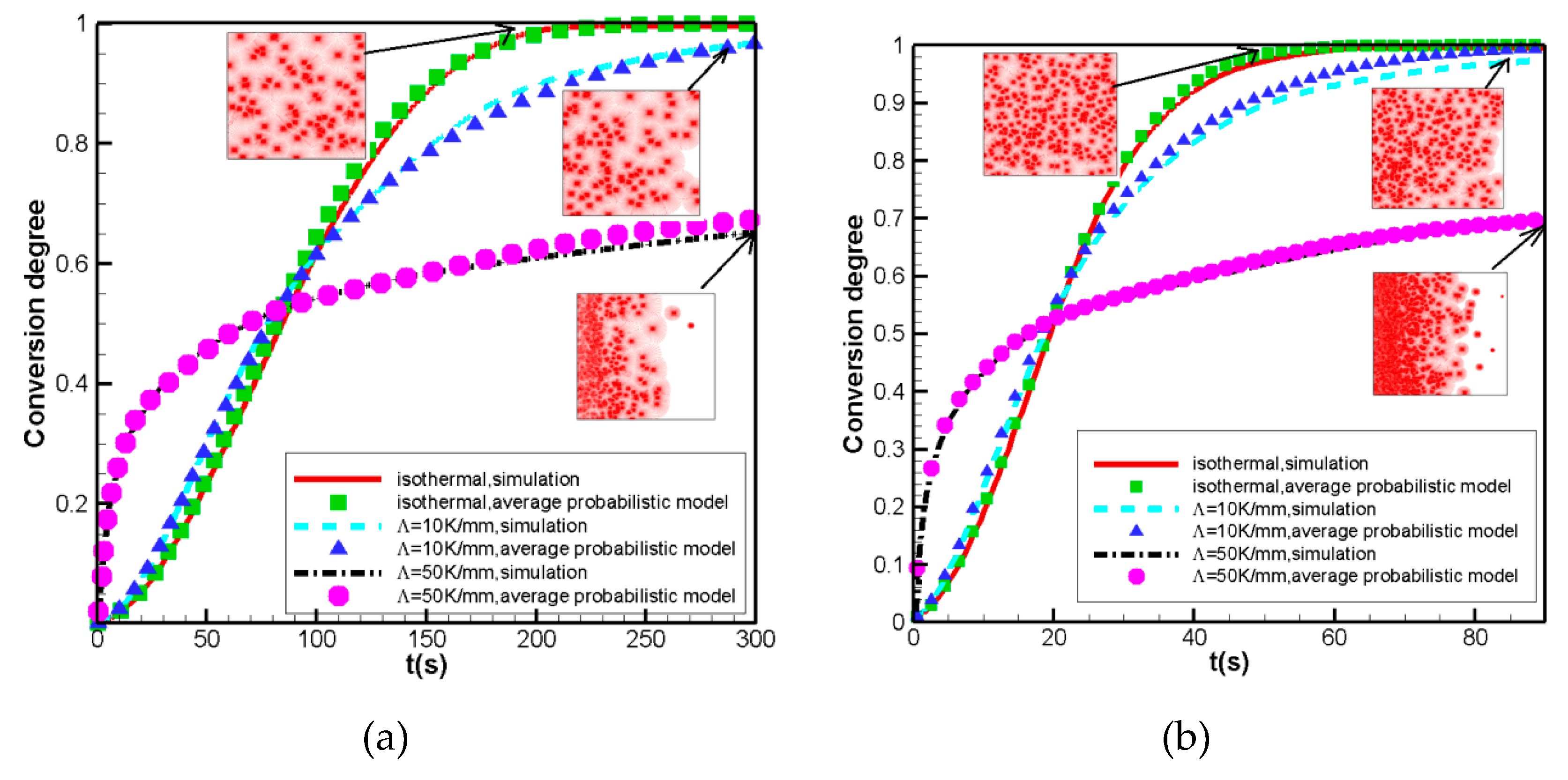
3.2.2. Performance of the Average Probabilistic Model

We now examine the performance of the average probabilistic model under three nucleation density distributions. Here, we set m = 6.

Nucleation Density Obeys Uniform Distribution

Figure 8 plots the conversion degree of the melt into spherulites between the Monte Carlo method and the average probabilistic model with $D=100/{\mathrm{mm}}^2$ and $D=1000/{\mathrm{mm}}^2$ where the nucleation density obeys uniform distribution. It is clear that the performance of the average probabilistic model is satisfied when the temperature gradient is less than $\mathsf{\Lambda }=50 \mathrm{K}/\mathrm{mm}$.

Nucleation Density Obeys a Linear Relationship with the Normal Growth Rate

Figure 9 shows the comparison of the conversion degree of the melt into spherulites between the Monte Carlo method and the average probabilistic model when nucleation density obeys a linear relationship with the normal growth rate: $D=B\times G_n$. Here, the value of $B$ is the same as in Section 3.1.2. As can be seen from the figure, the average probabilistic model shows good agreement with the Monte Carlo method when the temperature gradient less than $\mathsf{\Lambda }=50 \mathrm{K}/\mathrm{mm}$.

Nucleation Density Obeys an Exponential Relationship between Temperatures

Figure 10 displays the comparison of the conversion degree of the melt into spherulites between the Monte Carlo method and the average probabilistic model under the condition that the nucleation density obeys an exponential relationship between temperatures. It is obvious that the average probabilistic model also does a good job.

3.2.3. Effects of Division Number m on the Conversion Degree When Using the Average Probabilistic Model

As shown in Section 3.2.2, the average probabilistic model performs well in predicting the crystallization conversion for three nucleation density distributions when m = 6. We now examine the effects of the division number m.

It is noted that the probabilistic model is still used to calculate the conversion degree of the melt into spherulites in a small part. However, there are still differences in temperature in this small area. If the differences are large, the non-uniformity of the nucleation density and the anisotropy of the growth of spherulites will lead to an inaccurate result. The appropriate choice of the division number, m, is therefore important.

We only consider the case when the nucleation density obeys an exponential relationship between temperatures because it is more relevant to the industry.

We define the following error, namely,

$$L_1-\mathrm{error}=\frac{1}{t_{end}}{\displaystyle \underset{0}{\overset{t_{end}}{\int }}|{\alpha }_{AP}-{\alpha }_{MC}|}dt$$

(18)

Here, ${\alpha }_{AP}$ is the conversion degree of the melt into spherulites predicted by the average probabilistic model, ${\alpha }_{MC}$ is the conversion degree of the melt into spherulites predicted by the Monte Carlo method, and $t_{end}$ is the crystallization time.

Table 1. $L_1-\mathrm{error}$ with different $\mathsf{\Lambda }$ and m when $T_0=120$ °C.

Λ\m	$\mathit{m}=1$	$\mathit{m}=2$	$\mathit{m}=3$	$\mathit{m}=6$
$\mathsf{\Lambda }=10 \mathrm{K}/\mathrm{mm}$	8.17749 × 10−2	3.41766 × 10−2	2.34258 × 10−2	1.72930 × 10−2
$\mathsf{\Lambda }=20 \mathrm{K}/\mathrm{mm}$	1.99437 × 10−1	6.19496 × 10−2	2.60574 × 10−2	5.49196 × 10−3
$\mathsf{\Lambda }=30 \mathrm{K}/\mathrm{mm}$	2.94745 × 10−1	6.96178 × 10−2	1.84072 × 10−2	8.83252 × 10−3
$\mathsf{\Lambda }=40 \mathrm{K}/\mathrm{mm}$	3.61451 × 10−1	9.02186 × 10−2	3.16783 × 10−2	3.04310 × 10−3
$\mathsf{\Lambda }=50 \mathrm{K}/\mathrm{mm}$	3.99903 × 10−1	7.89859 × 10−2	4.75056 × 10−2	5.82306 × 10−3

shows the $L_1-\mathrm{error}$ with different temperature gradients and different division numbers, m, at the central temperature $T_0=120$ °C. The crystallization time is set to $t_{end}=90$ s. It can be seen that the $L_1-\mathrm{error}$ decreases with increasing division number, m. In fact, with the increase of the division number, m, the temperature difference in the small part decreases. This reduces the non-uniformity of the nucleation density and the growth anisotropy of the spherulites. Thus, the probabilistic model in the small part becomes more accurate. If the $L_1-\mathrm{error}$ remains within 5%, the division number, m, should be at least 2 in the case of $\mathsf{\Lambda }=10 \mathrm{K}/\mathrm{mm}$ and at least 3 in the case of $\mathsf{\Lambda }=20 \mathrm{K}/\mathrm{mm}~50 \mathrm{K}/\mathrm{mm}$. It should be pointed out that the minimum division number, m, is related to the overall size of the sample, the central temperature, and the temperature gradients.

Table 2. $L_1-\mathrm{error}$ with different $T_0$ and $\mathsf{\Lambda }$ values when m = 6.

Λ\T0	${\mathit{T}}_0=125$ °C	${\mathit{T}}_0=120$ °C	${\mathit{T}}_0=115$ °C	${\mathit{T}}_0=110$ °C
$\mathsf{\Lambda }=10 \mathrm{K}/\mathrm{mm}$	7.24991 × 10−3	1.72930 × 10−2	6.03332 × 10−3	2.89613 × 10−3
$\mathsf{\Lambda }=20 \mathrm{K}/\mathrm{mm}$	1.21956 × 10−2	5.49196 × 10−3	6.49543 × 10−3	2.42921 × 10−3
$\mathsf{\Lambda }=30 \mathrm{K}/\mathrm{mm}$	1.05234 × 10−2	8.83252 × 10−3	7.60522 × 10−3	4.33847 × 10−3
$\mathsf{\Lambda }=40 \mathrm{K}/\mathrm{mm}$	6.36686 × 10−3	3.04310 × 10−3	9.75746 × 10−3	8.50667 × 10−3
$\mathsf{\Lambda }=50 \mathrm{K}/\mathrm{mm}$	9.21316 × 10−3	5.82306 × 10−3	9.06534 × 10−3	3.86348 × 10−3

lists the $L_1-\mathrm{error}$ values of the average probabilistic model with different central temperatures and temperature gradients when $m=6$. The crystallization time are $t_{end}=300 \mathrm{s}, 90 \mathrm{s}, 60 \mathrm{s}, 60 \mathrm{s}$ when $T_0=$ 125 °C, 120 °C, 115 °C, 110 °C, respectively. It can be seen from Table 2 that when the central temperature $T_0\le$ 125 °C and the temperature gradient $\mathsf{\Lambda }\le 50 \mathrm{K}/\mathrm{mm}$, the $L_1-\mathrm{error}$ is less than 2%. Thus, in this study, when $m=6$, the good solution is obtained.

4. Conclusions

We have conducted a thorough investigation of the probabilistic model under temperature gradients. The polymer iPP was chosen as a model polymer with which to study the performance of the probabilistic model in predicting the overall crystallization kinetics compared with the Monte Carlo method. Conclusions are drawn as follows:

(1) For parts with large temperature gradients and large temperature differences, the correct solution cannot be obtained by using the probabilistic model directly. In fact, the model is greatly affected by the non-uniformity of the nucleation density. The more non-uniform the nucleation density distribution, the worse the prediction of the conversion degree by the probabilistic model. Besides, a large temperature gradient and a large temperature difference increase the growth anisotropy of the spherulites, and thus the predictions of the probabilistic model become worse.

(2) The average probabilistic model gives better results than the probabilistic model used directly. The larger the division number, the better the effect of the average probabilistic model because the non-uniformity of the nucleation density and the growth anisotropy of the spherulites are reduced.

We hope this study will give more insight into the understanding of the crystallization kinetics model under temperature gradients.

References

1. Kennedy, P.; Zheng, R. Flow Analysis of Injection Molds, 2nd ed.; Hanser: Munich, Germany, 2013. [Google Scholar]
2. Pantanin, R.; Coccorullo, I.; Speranza, V. Modeling of morphology evolution in the injection molding process of thermoplastic polymers. Prog. Polym. Sci. 2005, 30, 1185–1222. [Google Scholar] [CrossRef]
3. Liu, Z.; Ouyang, J.; Ruan, C.; Liu, Q. Simulation of polymer crystallization under isothermal and temperature gradient condtions using praticle level set method. Crystals 2016, 6, 90. [Google Scholar] [CrossRef]
4. Piorkowska, E.; Galeski, A. Overall crystallization kinetics. In Handbook of Polymer Crystallization; Piorkowska, E., Rutledge, G.C., Eds.; Jonn Wiley & Sons Inc.: Hoboken, NJ, USA, 2013; pp. 215–234. [Google Scholar]
5. Piorkowska, E. Modeling of polymer crystallization in temperature gradient. J. Appl. Polym. Sci. 2002, 86, 1351–1362. [Google Scholar] [CrossRef]
6. Avrami, M. Kinetics of phase change. I. General theory. J. Chem. Phys. 1939, 7, 1103–1112. [Google Scholar]
7. Pawlak, A.; Piorkowska, E. Crystallization of isotactic polypropylene in a temperature gradient. Colloid. Polym. Sci. 2001, 279, 939–946. [Google Scholar] [CrossRef]
8. Ruan, C. Morphological monte carlo simulation for crystallzation of isotactic polypropylene in a temperature gradient. Crystals 2019, 9, 213. [Google Scholar] [CrossRef]
9. Liu, P.; Hu, A.; Wang, S.; Shi, M.; Ye, G.; Xu, J. Evaluation of nonisothermal crystallization kinetics models for linear poly(phenylene sulfide). J. Appl. Polym. Sci. 2011, 121, 14–20. [Google Scholar] [CrossRef]
10. Yang, J.; McCoy, B.; Madras, G. Distribution kinetics of polymer crystallization and the Avrami equation. J. Chem. Phys. 2005, 122, 064901. [Google Scholar] [CrossRef] [PubMed]
11. Zhou, Y.; Wu, W.; Lu, G.; Zou, J. Isothermal and non-isothermal crystallization kinetics and predictive modeling in the solidification of poly(cyclohexylene dimethylene cyclohexanedicarboxylate) melt. J. Elast. Plast. 2016, 49, 132–156. [Google Scholar] [CrossRef]
12. Goff, R.; Poutot, G.; Delaunay, D.; Fulchiron, R.; Koscher, E. Study and modeling of heat transfer during the solidification of semi-crystalline polymers. Int. J. Heat Mass Transf. 2005, 48, 5417–5430. [Google Scholar] [CrossRef]
13. Yan, D.; Jiang, H.; Li, H. FEM simulation of nonisothermal crystallization, 1 crystallinity distribution on 2D space. Macromol. Theory Simul. 2000, 9, 166–175. [Google Scholar] [CrossRef]
14. Zhou, Y.; Turng, L.; Shen, C. Modeling and prediction of morphology and crystallinity for cylindrical-shaped crystals during polymer processing. Polym. Eng. Sci. 2010, 50, 1226–1235. [Google Scholar] [CrossRef]
15. Lamberti, G.; Santis, F. Heat transfer and crystallization kinetics during fast cooling o of thin polymer films. Heat Mass Transf. 2007, 43, 1143–1150. [Google Scholar] [CrossRef]
16. Hoffman, J.; Miller, R. Kinetics of crystallization from the melt and chain folding in polyethylene fractions revisited: Theory and experiment. Polymer 1997, 38, 3151–3212. [Google Scholar] [CrossRef]
17. Swaminarayan, S.; Charbon, C. A multiscale model for polymer crystallization. I. Growth of individual spherulites. Polym. Eng. Sci. 1998, 38, 634–643. [Google Scholar]
18. Thananchai, L. Mathematical modeling of solidification of semi-crystallization polymers under quiescent non-isothermal crystallization: Determination of crystallite’s size. Sci. Asia. 2001, 27, 127–132. [Google Scholar]
19. Ruan, C. Kinetics and morphology of flow indueced polymer crystallization in 3D shear flow investigated by Monte Carlo simulation. Crystals 2017, 7, 51. [Google Scholar] [CrossRef]
20. Ruan, C.; Liu, C.; Zheng, G. Monte Carlo simulation for the morphology and kinetics of spherulites and shish-kebabs in isothermal polymer crystallization. Math. Prob. Eng. 2015, 50624, 1–10. [Google Scholar] [CrossRef]
Figure 1. Growth morphology of a single crystal.
Crystals 09 00538 g001
Figure 2. Crystal morphology predicted by the Monte Carlo method: (a) D = 100 / mm 2 ; (b) D = 1000 / mm 2 .
Crystals 09 00538 g002
Figure 3. Comparison of conversion degree of the melt into spherulites between the Monte Carlo method and the probabilistic model: (a) D = 100 / mm 2 ; (b) D = 1000 / mm 2 .
Crystals 09 00538 g003
Figure 4. Crystal morphology predicted by the Monte Carlo method: (a) D = 100 / mm 2 ; (b) D = 1000 / mm 2 .
Crystals 09 00538 g004
Figure 5. Comparison of conversion degree of the melt into spherulites between the Monte Carlo method and the probabilistic model: (a) D = 100 / mm 2 ; (b) D = 1000 / mm 2 .
Crystals 09 00538 g005
Figure 6. Crystal morphology predicted by the Monte Carlo method: (a) T 0 = 125 °C; (b) T 0 = 120 °C.
Crystals 09 00538 g006
Figure 7. Comparison of conversion degree of the melt into spherulites between the Monte Carlo method and the probabilistic model: (a) T 0 = 125 °C; (b) T 0 = 120 °C.
Crystals 09 00538 g007
Figure 8. Comparison of conversion degree of the melt into spherulites between the Monte Carlo method and the average probabilistic model: (a) D = 100 / mm 2 ; (b) D = 1000 / mm 2 .
Crystals 09 00538 g008
Figure 9. Comparison of conversion degree of the melt into spherulites between the Monte Carlo method and the average probabilistic model: (a) D = 100 / mm 2 ; (b) D = 1000 / mm 2 .
Crystals 09 00538 g009
Figure 10. Comparison of conversion degree of the melt into spherulites between the Monte Carlo method and the average probabilistic model: (a) T 0 = 125 °C; (b) T 0 = 120 °C.
Crystals 09 00538 g010