Twisted Graphene Bilayers and Quasicrystals: A Cut and Projection Approach

Abstract

In this work, a modified version of the cut and projection approach is proposed to describe the structure of graphene bilayers with twist angles. With this method, the rotation between two graphene layers is viewed as a rotation of the projection space and the resulting projected structure is interpreted as the set of points of best fit between the two rotated structures. Additionally, focus is given to the pertinence of the many algebraic and geometric tools used in grain boundaries and in quasicrystals to graphene bilayer system (or any other bilayer system, for that matter) case.

1. Introduction

During the last years, the possibility of tailoring heterostructures by piling up several two-dimensional materials has become a reality [1,2]. Such structures are not only important for technological applications [1] but also serve as a playground to observe new and exotic phases of matter [3,4]. Among such phases, we can cite the observation of the Hofstadter butterfly fractal spectrum and its associated topological states. Such experiment was made by using a moiré pattern of graphene over graphene [5]. More recently, a phase-diagram akin to those seen in complex high-$T_c$ superconductor materials has been observed in graphene over twisted graphene at certain magical rotation angles [6]. Moreover, recent advances in controlling the rotation angle of graphene over graphene [7] allows using it as an effective knob for tuning their electronic properties [8]. Although these results are not fully understood at the moment, recent theoretical advances are based either on Hubbard Hamiltonians [9] or Dirac Hamiltonians with an emergent effective potential for electrons [10]. In any case, there are many open questions concerning the electronic and optical properties of 2D heterostructures which require adequate tools to describe their structure [3,11].

A typical example of the involved complexity is the actual determination of the lattice parameter of the moiré superlattice. For example, in graphene on Ir(1 1 1), obtained via a pyrolytic cleavage of ethylene [12,13], there is a slight lattice mismatch between the graphene and Ir(1 1 1) lattices, resulting in a moiré pattern with a repeat distance of 2.53 nm [12]. However, refinements indicated that this was just an excellent approximation, since the actual structure comprises three beatings instead of two [14].

Moreover, until recently most work has dealt with the commensurate case, that is, when two layers form a supercell, what in materials science is known as a coincidence site lattice. Consider that one of the layers $L_1$ is hexagonal and spanned by $\{a_1,a_2\}$ and the other $L_2$ by $\{a_3,a_4\}$ and $L_2$ can be obtained from $L_1$ by means of a rotation through an angle $\theta$. Then, a discrete coincidence site lattice, $L_1\cap L_2$, exists only when $\theta$ satisfies,

$$cos\theta =\frac{n^2+4mn+m^2}{2(n^2+mn+m^2)}$$

(1)

for integers m and n. In the materials science and crystallographic literature, an equivalent condition,

$$tan(\theta /2)=\frac{\mid m-n\mid }{\sqrt{3}(m+n)}=\frac{\sqrt{3}\mid m-n\mid }{3(m+n)}=\sqrt{3}\frac{p}{q},$$

is used, where p and q are integers [15]. Both can be derived using the methods described first by Ranganathan [16], however the latter form involving half angles is in better agreement with the spinorial (Rodrigues vector, quaternions, and Cayley–Klein parameters) character of the rotation involved [15,17].

Researchers in the 2D matter community field frequently refer to moiré patterns, but no one has recalled that moiré patterns in (periodic or not) structures are related to Bollmann’s O-lattice concept [18]. Here, we describe this tool. In fact, the need for such tools is becoming evident as, for example, very recently it has been claimed that there is an incommensurate heterostructure analog to a quasicrystal [11], obtained by growing a quasicrystalline 30${}^{\circ }$ twisted bilayer graphene (30${}^{\circ }$-tBLG), stabilized by a Pt(111) substrate [11]. Beside this experiment, the 30${}^{\circ }$ quasicrystalline twisted bilayer graphene was simultaneously discovered by Ahn, Sung Joon, et al. [19]. There are now available some theoretical works to model such system [20,21]. The observed quasiperiodic order is predicted to exhibit quantum oscillations associated to exotic spiral Fermi surfaces [22].

The aim of this paper is twofold: first, to clarify and present the tools necessary to describe such kind of heterostructures and, second, to develop a cut and projection approach to obtain the best fit lattice between two rotated graphene structures. One can claim that no such concepts are needed as a moiré pattern seems to be just a superposition of two lattices. However, the superposition of the lattices results in a modulation of the graphene sheet as strain needs to be minimized [3,10]. Thus, there is a deformation strain field which modulates the equilibrium position of atoms on each graphene layer [3]. This follows the spirit of one of the oldest known quasiperiodic Hamiltonians: the Frenkel–Kontorova model [23]. Moreover, all particles and quasiparticles, such as electrons or holes, feel an effective potential which is the sum of both deformed and modulated lattices [10]. Such deformation field has a paramount importance to the observed superconductivity at magic angles [8]. Thus, our approach here is in the spirit of the Frenkel–Kontorova scenario: an effective two-dimensional model.

The structure of this paper is as follows. In Section 2, we provide some general remarks concerning the crystallography of graphene, including coincidence lattices and Bollmann’s O-lattice and point out its presence in the bilayers. The cut and projection method is applied to the generation of bilayers in Section 3. A discussion and our conclusions are presented in Section 4.

2. General Considerations

In this section, some general tools to describe bilayers are presented, in particular those that have not yet been used in this field and can be useful. Here, we consider two graphene sheets, one on top of the other, having the origin in common and rotated through an angle $\theta$. The underlying lattice $L_1$ for a graphene layer is hexagonal. We take as lattice vectors,

$${\mathbf{a}}_1=a\left(\frac{\sqrt{3}}{2},-\frac{1}{2}\right)\mathrm{and}{\mathbf{a}}_2=a\left(\frac{\sqrt{3}}{2},\frac{1}{2}\right),$$

(2)

with respect to an orthonormal basis of ${\mathbb{R}}^2$. Here, a is the lattice parameter for graphene. Other choices of primitive vectors are possible and have been used in the literature [15]. Notice that here we work already with only one layer, as our aim is to define an effective 2D lattice, yet the results are easily extended to bilayers by adding a new coordinate.

The rotated lattice ($L_2$) can be obtained by rotating $L_1$ through an angle $\theta$. The rotation matrix is given by

$$R_{\theta }=\left[\begin{array}{cc}cos\theta & -sin\theta \\ sin\theta & cos\theta \end{array}\right].$$

Frequently, we work in terms of the so-called structure matrices, that is, matrices having as columns the Cartesian components of the primitive lattice vectors. For $L_1$, the structure matrix is

$$S_1=\frac{a}{2}\left[\begin{array}{cc}\sqrt{3}& \sqrt{3}\\ -1& 1\end{array}\right],$$

whereas the structure matrix for $L_2$ is

$$S_2=\frac{a}{2}\left(\begin{array}{cc}sin\theta +\sqrt{3}cos\theta & \sqrt{3}cos\theta -sin\theta \\ \sqrt{3}sin\theta -cos\theta & cos\theta +\sqrt{3}sin\theta \end{array}\right).$$

The structure matrix for the reciprocal lattice ($L_1^{*}$) is

$$S_1^{*}=\frac{1}{a}\left[\begin{array}{cc}\frac{1}{\sqrt{3}}& \frac{1}{\sqrt{3}}\\ -1& 1\end{array}\right],$$

whereas that for $L_2^{*}$ is

$$S_2^{*}=\frac{1}{a}\left(\begin{array}{cc}\frac{1}{\sqrt{3}}cos\theta +sin\theta & \frac{1}{\sqrt{3}}sin\theta -cos\theta \\ \frac{1}{\sqrt{3}}cos\theta -sin\theta & \frac{1}{\sqrt{3}}sin\theta -cos\theta \end{array}\right).$$

2.1. O Points

When two 2D lattices are superimposed, the emergence of the moiré structure can be described by means of the O-lattice concept developed by Bollmann [18]. The O points are all those points such that $L_2$ can be obtained from $L_1$ by the same rotation through $\theta$.

The rotation $R_{\theta }$ through an angle $\theta$ can be represented as multiplication by the complex number (of course a full equivalent matrix treatment can be given) $R_{\theta }=e^{i\theta }$, thus Bollmann’s equation for O-lattice points (O) reads $\left(I-R_{\theta }^{-1}\right)O={\mathbf{l}}_1$, where ${\mathbf{l}}_1\in L_1$. Therefore,

$$O=\frac{{\mathbf{l}}_1}{\left(1-e^{-i\theta }\right)}=\frac{{\mathbf{l}}_1}{2}\left[\frac{\left(1-cos\theta -isin\theta \right)}{1-cos\theta }\right].$$

Using some standard trigonometric identities, we get

$$O=\frac{{\mathbf{l}}_1}{2}\left[1-\frac{i}{tan(\theta /2)}\right],$$

which, of course, could be re-cast in matrix notation using the fact that multiplication by i is a rotation by $\pi /2$, to obtain

$$O=\left[I-\frac{1}{tan(\theta /2)}{R}_{\pi /2}\right]\frac{{\mathbf{l}}_1}{2},$$

where I is the $2\times 2$ identity matrix.

In Figure 1, we show two graphene layers rotated $\theta ={13.17}^{\circ }$, a commensurate case where there is a superlattice. Figure 1 also shows two layer rotated by $\theta ={30}^{\circ }$, producing a dodecagonal structure. In both cases, one can visually detect the O-points as “rosettes”. The O-points form a lattice even in non-commensurate cases.

2.2. Reciprocity and DSC Lattice

If $L_1$ and $L_2$ are two lattices, in general, $L_1\cap L_2$ will not be a discrete lattice. If $L_1$ is spanned by the vectors $\{{\mathbf{a}}_1,{\mathbf{a}}_2\}$ and $L_2$ is spanned by $\{{\mathbf{b}}_1,{\mathbf{b}}_2\}$, there will be a discrete lattice if and only if

$${\mathbf{a}}_i=\sum _{j=1}^2{M}_{ji}{\mathbf{b}}_j,$$

for an invertible rational matrix M (transition matrix). The expressions given in Equation (1), in terms of m and n, are special cases to be used when the transition matrix is a rotation.

The lattice

$$L_1+L_2=\{\mathbf{a}+\mathbf{b}\mid \mathbf{a}\in L_1,\mathbf{b}\in L_2\}$$

is called DSC lattice, or sum lattice, and it is a discrete lattice if and only if $L_1\cap L_2$ is discrete.

In the latter case, the following duality relationships hold

$$\begin{array}{cc}\hfill {\left(L_1\cap L_2\right)}^{*}& =L_1^{*}+L_2^{*}\hfill \\ \hfill {\left(L_1+L_2\right)}^{*}& =L_1^{*}\cap L_2^{*}.\hfill \end{array}$$

In bilayers, these relations can clarify the relationships between various quantities. The reciprocal lattice of the superlattice (CSL) consists of sums (and differences) of reciprocal vectors of the two underlying lattices. Thus far, these concepts have not been used in the literature on graphite bilayers, even though they appear in most of the literature on grain boundaries. The purpose of this summary is to turn the attention to these concepts and results that can be of help in the exciting field of graphene bilayers. It should also be mentioned that a theory of interfaces that uses a modified version of the projection methods has been developed [24].

In the next section, we adapt the cut and projection method, extensively used in the field of quasicrystals, to obtain the best fit structure, or an effective structure, produced when two graphene layers are rotated by a certain angle. In Ref. [17], the problem of two rotated squared lattices was worked out by projecting from a four-dimensional lattice. In this work, a further modification of the method is required since first a honeycomb structure (instead of the hexagonal lattice) must be obtained by the projection method.

3. Cut and Projection Approach

A powerful tool to describe modulated crystals and quasicrystals is the cut and projection method. In this section, we adapt this method to describe rotated layers. For the sake of completeness, let us briefly review such method restricted to quasiperiodic tilings of the plane. Under certain conditions (see below), a quasiperiodic tiling of the plane generated by linear integer combinations of the vectors $\{{\mathbf{a}}_1,{\mathbf{a}}_2,\dots ,{\mathbf{a}}_N\}$, $N>2$, can be obtained by projecting points from a N-dimensional hypercubic lattice ${\mathbb{Z}}^N\subset {\mathbb{R}}^N$ in the following way. Let $L={\mathbb{Z}}^N$ be the hypercubic lattice generated by the standard basis $\{{\mathbf{e}}_1,{\mathbf{e}}_2,\dots ,{\mathbf{e}}_N\}$ and let ${\Gamma }^N$ be the unitary hypercube. Let $E^{\Vert }$ be a two-dimensional subspace of ${\mathbb{R}}^N$ that does not contain any point of the lattice except the origin. An open strip $S=E^{\Vert }+{\Gamma }^N$ is defined and the projection onto $E^{\Vert }$ of all the points inside S gives a quasiperiodic tiling of the plane.

This projection formalism works provided that there exists a projector $P^{\Vert }:{\mathbb{R}}^N\to E^{\Vert }$ such that

$$P^{\Vert }\left({\mathbf{e}}_i\right)={\mathbf{a}}_i,i=1,\dots ,N.$$

(3)

The existence of $P^{\Vert }$ is guaranteed if the set $\{{\mathbf{a}}_1,{\mathbf{a}}_2,\dots ,{\mathbf{a}}_N\}$ forms a eutactic star [25,26]. The orthogonal projection of a set of orthogonal vectors in $R^N$ onto a two-dimensional space is called a eutactic star; if the vectors in $R^N$ are orthonormal, the projection is called a normalized eutactic star. In other words, if the set $\{{\mathbf{a}}_1,{\mathbf{a}}_2,\dots ,{\mathbf{a}}_N\}$ forms a normalized eutactic star, then there exists a projector $P^{\Vert }$ such that Equation (3) is fulfilled and actually:

$$P_{i,j}^{\Vert }={\mathbf{a}}_i·{\mathbf{a}}_j.$$

(4)

A necessary and sufficient condition for a star to be eutactic is due to H. Hadwiger [27]: a star $\left\{{\mathbf{a}}_1,{\mathbf{a}}_2,\dots {\mathbf{a}}_N\right\}$ in ${\mathbb{R}}^n$ is a normalized eutactic if and only if

$$\sum _{i=1}^N\left(\mathbf{x}·{\mathbf{a}}_i\right){\mathbf{a}}_i=\mathbf{x},$$

is fulfilled for all $\mathbf{x}\in {\mathbb{R}}^n$.

A more practical form of the eutacticity criterion is obtained if the structure matrix S is introduced. In this case, S is the matrix whose columns are the components of the vectors $\left\{{\mathbf{a}}_1,{\mathbf{a}}_2,\dots ,{\mathbf{a}}_N\right\}$, with respect to a given fixed orthonormal basis of ${\mathbb{R}}^n$. The matrix form of Hadwiger’s theorem sates that the star represented by S is normalized eutactic if and only if

$$S{S}^T=I,$$

(5)

where I is the $n\times n$ unit matrix.

To summarize, a quasiperiodic tiling of the plane generated by linear integer combinations of the vectors $\{{\mathbf{a}}_1,{\mathbf{a}}_2,\dots ,{\mathbf{a}}_N\}$, $N>2$, can be obtained by cut and projection from ${\mathbb{Z}}^N\subset {\mathbb{R}}^N$ if the set of vectors form a normalized eutactic star.

To adapt the cut and projection method to the case of graphene bilayers, consider first the case of two lattices in the plane, $L_1$ and $L_2$, rotated in between by a given angle $\theta$. Let $L_1$ and $L_2$ be generated by $\left\{{\mathbf{a}}_1,{\mathbf{a}}_3,{\mathbf{a}}_5\right\}$ and $\left\{{\mathbf{a}}_2,{\mathbf{a}}_4,{\mathbf{a}}_6\right\}$, respectively, and given by:

$$\begin{array}{cc}\hfill {\mathbf{a}}_1& =\{c,-s\},\hfill \\ \hfill {\mathbf{a}}_2& =\{c,s\},\hfill \\ \hfill {\mathbf{a}}_3& =\left\{\frac{\sqrt{3}}{2}s-\frac{1}{2}c,\frac{\sqrt{3}}{2}c+\frac{1}{2}s\right\},\hfill \\ \hfill {\mathbf{a}}_4& =\left\{-\frac{1}{2}c-\frac{\sqrt{3}}{2}s,\frac{\sqrt{3}}{2}c-\frac{1}{2}s\right\},\hfill \\ \hfill {\mathbf{a}}_5& =\left\{-\frac{1}{2}c-\frac{\sqrt{3}}{2}s,\frac{1}{2}s-\frac{\sqrt{3}}{2}c\right\},\hfill \\ \hfill {\mathbf{a}}_6& =\left\{\frac{\sqrt{3}}{2}s-\frac{1}{2}c,-\frac{\sqrt{3}}{2}c-\frac{1}{2}s\right\},\hfill \end{array}$$

(6)

where $c=cos\left(\varphi \right)/\sqrt{3}$ and $s=sin\left(\varphi \right)/\sqrt{3}$.

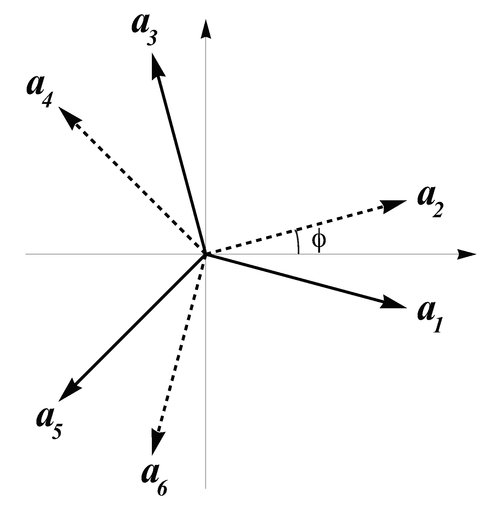
As shown in Figure 2, if $\varphi =0$, both vector sets collapse and three vectors pointing to the vertices of a triangle are obtained. If $\varphi ={15}^{\circ }$, six vectors pointing to six vectors of a dodecagon are obtained instead. Consequently, with linear integer combinations of the vectors in Equation (6), two hexagonal lattices rotated by $\theta =2\varphi$ can be generated.

With the vectors in Equation (6), the structure matrix is built as:

$$S=\left[{\mathbf{a}}_1\right|{\mathbf{a}}_2|\cdots |{\mathbf{a}}_6],$$

and it turns out that $S{S}^T=I$, that is, the star $\{{\mathbf{a}}_1,{\mathbf{a}}_2,\dots ,{\mathbf{a}}_6\}$ is eutactic for every value of $\theta$.

Notice that the vectors in Equation (6) depend on $\varphi$ hence, according to Equation (4), the projector $P^{\Vert }$ also depends on $\varphi$. As the column space of $P^{\Vert }$ is $E^{\Vert }$, then varying $\varphi$ is the same as projecting onto a rotating $E^{\Vert }$ space and this, in turn, can be interpreted as the rotation of the two lattices $L_1$ and $L_2$ in between by $\theta =2\varphi$. The cut and projection method under this situation can be interpreted as discussed in what follows.

As described in Ref. [17], for the case of square lattices, two rotated lattices can be viewed as a twin grain boundary and the GCSN (generalized coincidences sites networks) or good fit lattice can be obtained by means of the cut and projection method, using a tube instead of the standard strip. In the case of two hexagonal lattices, we should project from a six-dimensional hypercubic lattice equipped with the standard basis $\left\{{\mathbf{e}}_1,{\mathbf{e}}_2,{\mathbf{e}}_3,{\mathbf{e}}_4,{\mathbf{e}}_5,{\mathbf{e}}_6\right\}$. The projection matrix $P^{\Vert }$ has the property in Equation (3) and its entries are given by Equation (4), where the vectors of the star are Equation (6).

The main idea behind the approach in Ref. [17] is that, given two lattices rotated in between, a coincidence site lattice can be generated or not, depending on the rotation angle. Then, a generalization of the coincide lattice is proposed that consists in a geometrical array of points of good fit, defined through the concept of neighbors. We say that two lattice points ${\mathbf{l}}_1\in L_1$ and ${\mathbf{l}}_2\in L_2$ are neighbors if and only if

$${\mathbf{l}}_1,{\mathbf{l}}_2\in {\Lambda }_1\left({\mathbf{l}}_1\right)\cap {\Lambda }_2\left({\mathbf{l}}_2\right),$$

(7)

where ${\Lambda }_i\left({\mathbf{l}}_i\right)$ is the Voronoi polygon of the point ${\mathbf{l}}_i$ ($i=1,2$). The generalized model postulates that the best fit structure is a set G of points given by [17]:

$$\left\{\frac{{\mathbf{l}}_1+{\mathbf{l}}_2}{2}|{\mathbf{l}}_1,{\mathbf{l}}_2\in {\Lambda }_1\left({\mathbf{l}}_1\right)\cap {\Lambda }_2\left({\mathbf{l}}_2\right)\right\}.$$

(8)

That is, if two points ${\mathbf{l}}_1\in {\mathbf{L}}_1$ and ${\mathbf{l}}_2\in {\mathbf{L}}_2$ are neighbors, a point of good fit is located at the middle between ${\mathbf{l}}_1$ and ${\mathbf{l}}_1$.

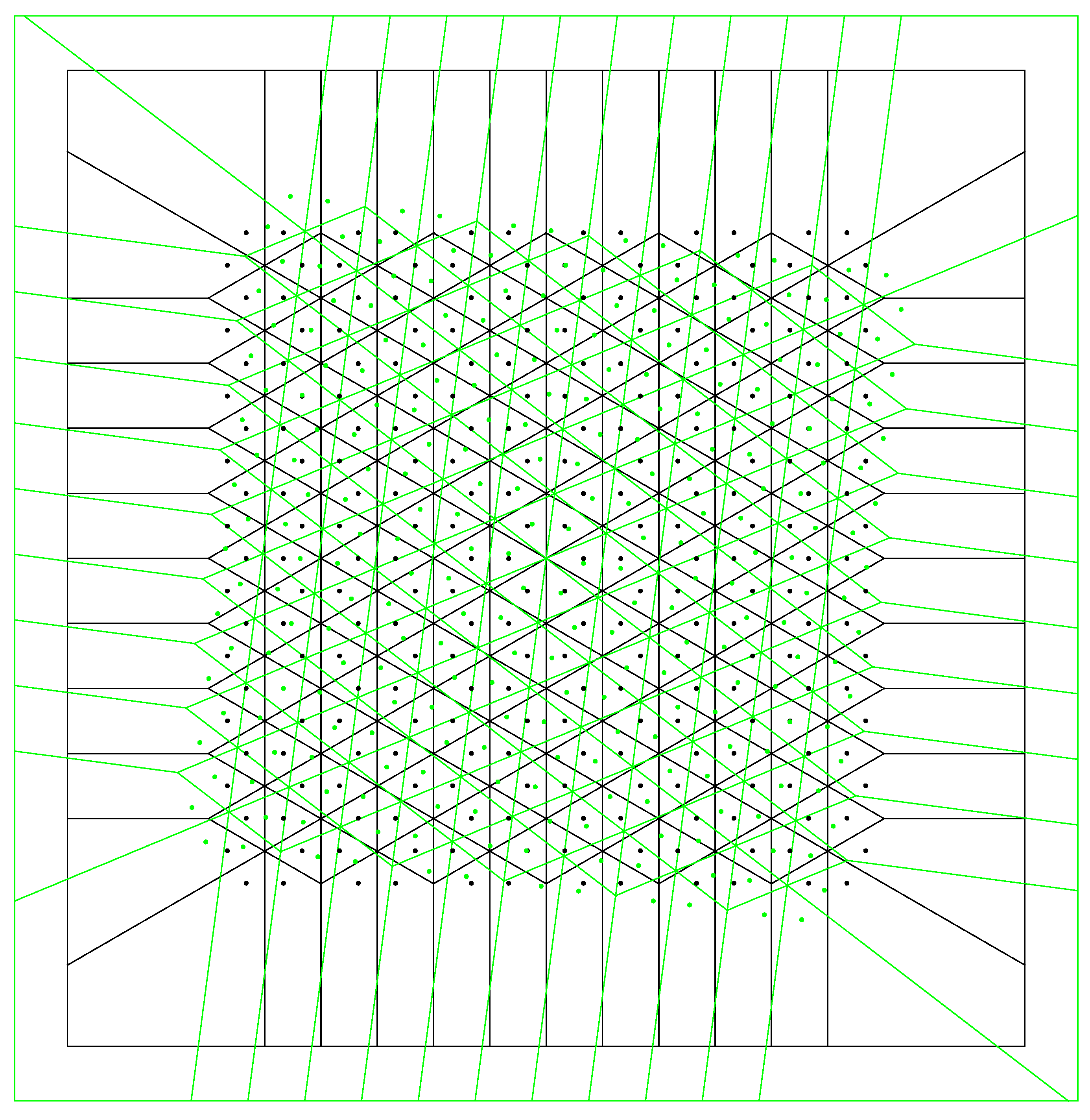
It should be stressed that, in our case, the hexagonal lattice and the honeycomb are dual to each other, that is the Voronoi tesselation of the honeycomb is the hexagonal lattice and vice versa. In Figure 3, two honeycomb structures rotated ${7.47}^{\circ }$ in between are shown with black and green points, respectively; the Voronoi tessellation associated to each lattice is also displayed in green and black lines. According to the procedure described above, we should look for neighbouring points, that is, where two points (one black and the other green) are both contained in the intersection of their respective Voronoi polyhedra. Neighbors points are then replaced by a point of good fit located at the middle.

In Ref. [17], it was shown that, given two lattices $L_1$ and $L_2$ rotated in between, the good fit lattice can be obtained by means of the cut and projection method, using a tube instead of the standard strip. Here, we adopt this approach but the way to determine the radius of the tube should be modified since the standard procedure will produce the best fit lattice associated to two rotated hexagonal lattices instead of two rotated honeycombs. As we shown below, the radius of the tube can be determined in order to obtain a honeycomb when $\varphi =0$, instead of the hexagonal lattice.

Consider the case of $\varphi =0$ in Equation (6), that is, the hexagonal lattice. In this case, ${\mathbf{a}}_1={\mathbf{a}}_2$, ${\mathbf{a}}_3={\mathbf{a}}_4$ and ${\mathbf{a}}_5={\mathbf{a}}_6$. The hexagonal lattice can be generated (in a redundant way) using, for instance, $\left\{{\mathbf{a}}_1,{\mathbf{a}}_3,{\mathbf{a}}_5\right\}$ or $\left\{{\mathbf{a}}_2,{\mathbf{a}}_4,{\mathbf{a}}_6\right\}$:

$$\mathbf{r}=\sum _{n_1,n_3,n_5}{n}_1{\mathbf{a}}_1+n_3{\mathbf{a}}_3+n_5{\mathbf{a}}_5.$$

(9)

By considering the vectors ${\delta }_1=\left({\mathbf{a}}_1-{\mathbf{a}}_5\right)/3$, ${\delta }_2=\left({\mathbf{a}}_3-{\mathbf{a}}_1\right)/3$ and ${\delta }_3=\left({\mathbf{a}}_5-{\mathbf{a}}_3\right)/3$, the honeycomb is generated as:

$$\mathbf{r}=\sum _{l=0}^1\sum _{n_1,n_3,n_5}{n}_1{\mathbf{a}}_1+n_3{\mathbf{a}}_3+n_5{\mathbf{a}}_5+l{\delta }_j,$$

(10)

where $j=1,2$ or 3. That is, the honeycomb is formed by an hexagonal lattice and a shifted copy of itself.

The space $E^{\left|\right|}$ is the row space of $P^{\left|\right|}$, for $\varphi =0$, which turns out to be:

$$E^{\left|\right|}=\mathrm{Span}\left\{(1,1,0,0,-1,-1),(0,0,1,1,-1,-1)\right\},$$

(11)

and the distance d of any lattice point $\mathbf{N}=(n_1,\dots ,n_6)$ to $E^{\left|\right|}$ is given by:

$$\begin{array}{ccc}9d^2\hfill & =& 2(n_1^2-n_1{n}_2+n_2^2)+2(n_3^2-n_3{n}_4+n_4^2)+2(n_5^2-n_5{n}_6+n_6^2)+\hfill \\ & & n_1(n_3+n_4+n_5+n_6)+n_2(n_3+n_4+n_5+n_6)+\hfill \\ & & n_3(n_5+n_6)+n_4(n_5+n_6).\hfill \end{array}$$

(12)

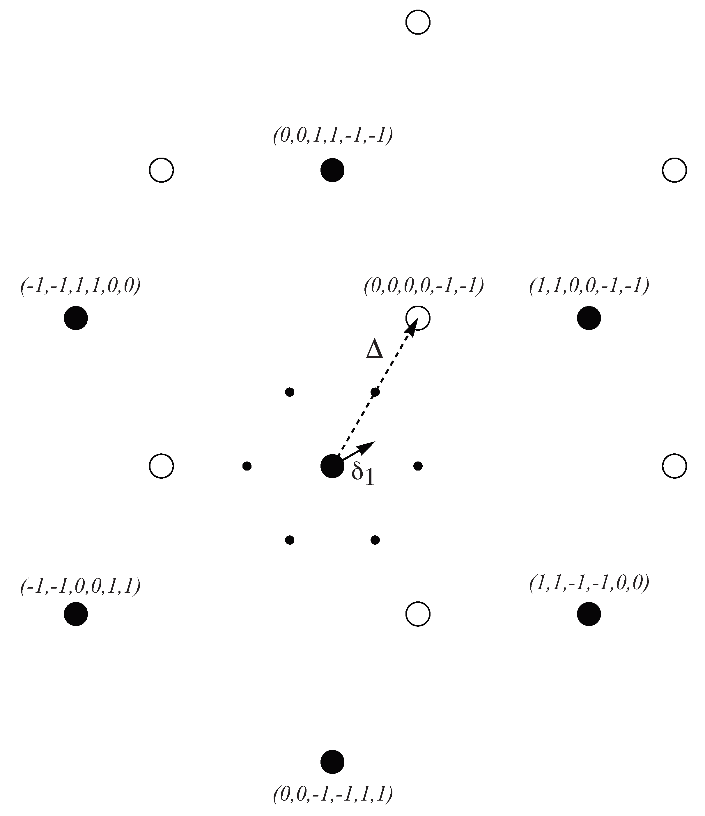
From this equation, we can verify that the vectors $(1,1,-1,-1,0,0)$, $(-1,-1,0,0,1,1)$, $(-1,-1,1,1,0,0)$, and $(0,0,-1-,1,1,1)$ belong to $E^{\left|\right|}$ (thus $d=0$), which together with the vectors in Equation (11) form a central hexagon (large disks in Figure 4). The distance from the vertices to the incenter of this hexagon is 2, which is $2\sqrt{3}$ larger than the hexagon generated by the standard basis vectors of ${\mathbb{R}}^6$ that are project onto Equation (6) and shown with small disks in Figure 4. Therefore, linear integer combinations of the vectors $(1,1,-1,-1,0,0)$, $(-1,-1,0,0,1,1)$, $(-1,-1,1,1,0,0),(0,0,-1,-1,1,1),(1,1,0,0,-1,-1)$, and $(0,0,1,1,-1,-1)$ generate the first hexagonal lattice, say A, which lie in $E^{\left|\right|}$, that is, the distance d of all its points is 0. Now, we now should obtain a second hexagonal lattice B, displaced by a vector $\Delta$ (dashed arrow in Figure 4). As in the case of ${\delta }_j$ in Equation (10), the magnitude of $\Delta$ is obtained as

$$∥\Delta ∥=∥P^{\Vert }\left((1,1,0,0,-1,-1)-(0,0,-1,-1,1,1)\right)∥/3=2/\sqrt{3},$$

and it can be verified that $\Delta$ is obtained by the projection of $(0,0,0,-1,-1)$ onto $E^{\left|\right|}$; actually, two other displacement vectors can be obtained by the projection of either $(-1,-1,0,0,0,0)$ or $(0,0,-1,-1,0,0)$. Any of these vectors are at a distance $\sqrt{2/3}\approx 0.816$ from $E^{\Vert }$, thus it seems that accepting points $\mathbf{N}$ such that $\parallel \mathbf{N}\parallel \le \sqrt{2/3}$ will produce the required A and B lattices. This is not the case, however; since the size of the vectors $\parallel {\mathbf{a}}_i\parallel$ in Equation (6) is $1/\sqrt{3}\approx 0.57$, the projection method will include the basis vectors of ${\mathbb{R}}^n$, which project onto an small hexagonal lattice, as shown with small disks in Figure 4. These points can be excluded by a translation of $E^{\Vert }$ along the $(-1,-1,-1,-1,-1,-1)$ direction. Thus, for instance with a translation by $(-\epsilon ,-\epsilon ,-\epsilon ,-\epsilon ,-\epsilon ,-\epsilon )$, the basis vectors have distances to $E^{\left|\right|}$ given by $d_1=\sqrt{2/3+2\epsilon +6{\epsilon }^2}$ while vectors such as $(-1,-1,0,0,0,0)$ have distances to $E^{\left|\right|}$ given by $d_2=\sqrt{2/3-4\epsilon +6{\epsilon }^2}$. Consequently, by translating $E^{\left|\right|}$ by $(-\epsilon ,-\epsilon ,-\epsilon ,-\epsilon ,-\epsilon ,-\epsilon )$ and accepting points such that $\parallel N\parallel \le \sqrt{2/3-4\epsilon +6{\epsilon }^2}$ will produce the required bipartite lattice.

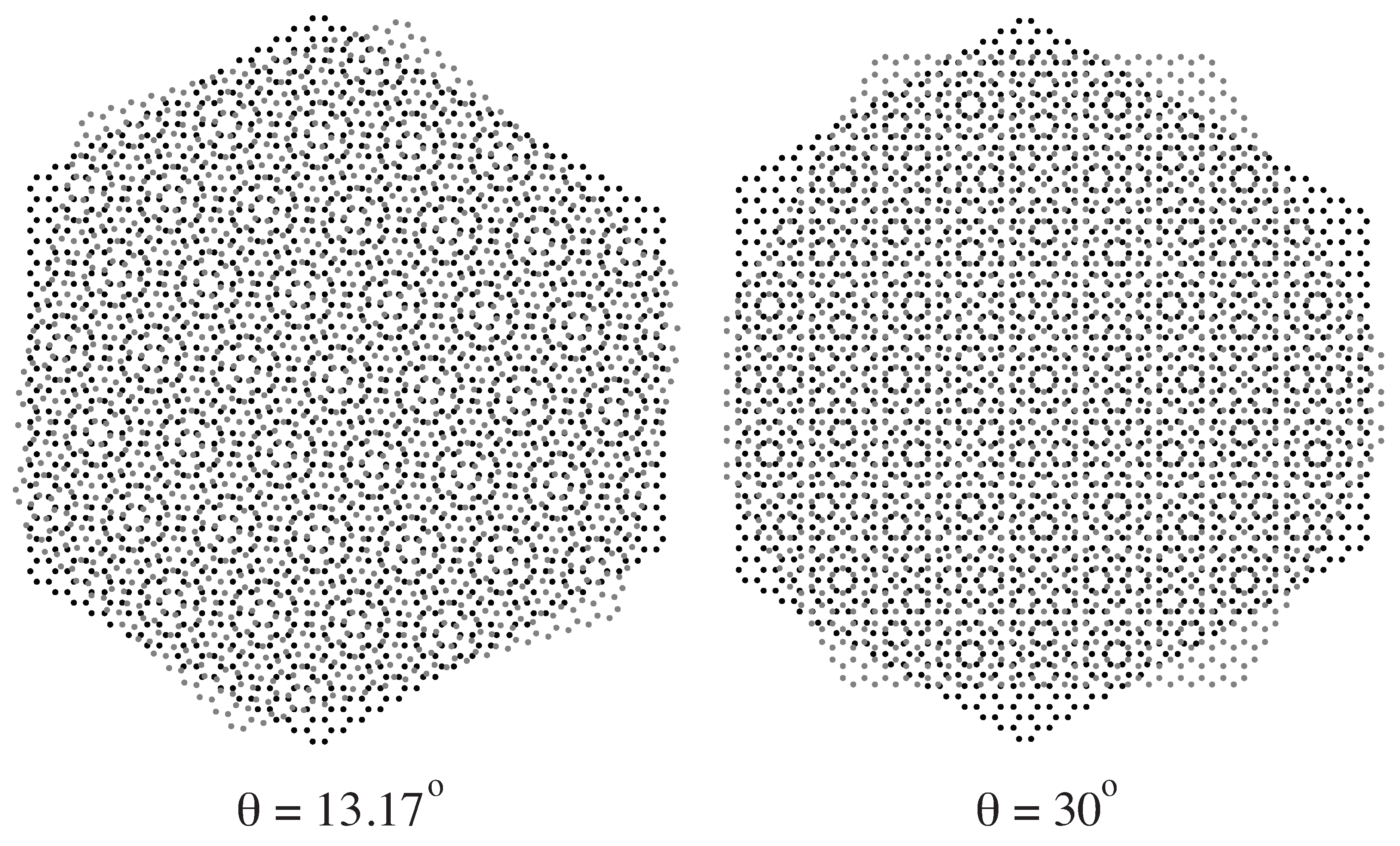
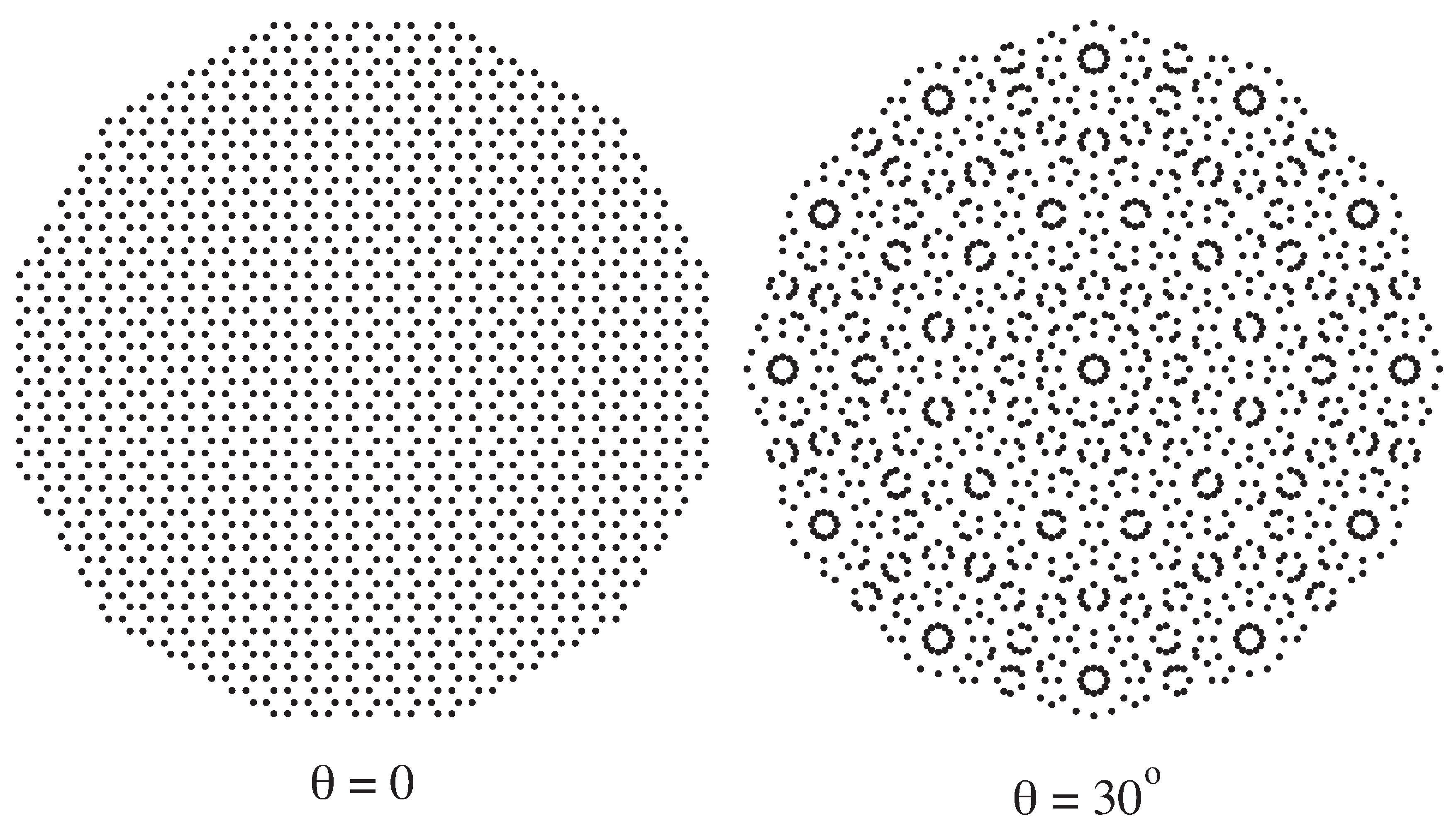
The utility of this approach is that, once the honeycomb lattices are obtained by projection, the space $E^{\left|\right|}$ can be rotated and the projected structure is transformed from periodic (honeycomb) to quasiperiodic with dodecagonal symmetry.

Some projection structures obtained when $E^{\left|\right|}$ is rotated are now shown. Consider a translation of $E^{\left|\right|}$ by $\epsilon =0.5$; in this case, we get $d_1=1.779$ and $d_2=0.4082$. In Figure 5 and Figure 6, we show projected structures obtained using a tube with radius $0.55$ ($<d_1$). 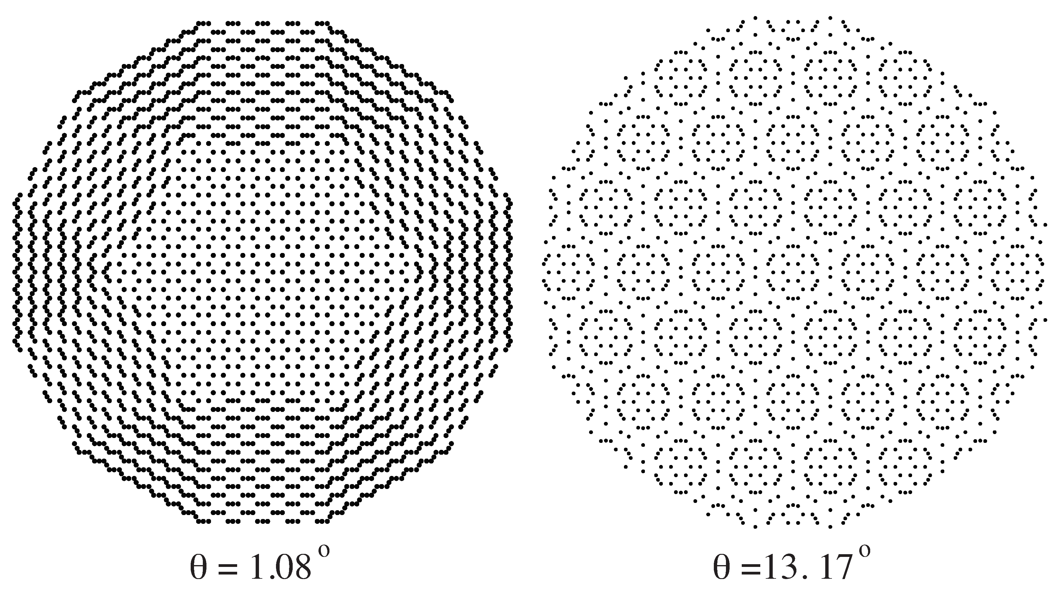The honeycomb for the case $\theta =0$ and a dodecagonal quasiperiodic structure when $\theta ={30}^{\circ }$ ($\varphi ={15}^{\circ }$) are shown in Figure 5, and two structures corresponding to $\theta ={1.08}^{\circ }$ (the golden angle) and $\theta ={13.17}^{\circ }$ are shown in Figure 6 (compare with Figure 1).

4. Discussion and Conclusions

As shown in Figure 5 and Figure 6, many types of lattices can be obtained and described by this approach. These coincidence patterns have paramount importance for the electronic properties. It has been experimentally observed that maximal coincidence regions represent maximal electron density probability regions [8,28]. Coincidence regions are where the flat bands, responsible for the strong electron–electron interaction, predominately localize [8]. As anticipated in the Introduction, strain and disorder play important roles in observing correlated states [8]. Despite this, our approach allows identifying coincidence points in a general scheme and therefore is very well suited to describe and produce effective renormalized Hamiltonians [10,29]. Moreover, the Fourier transform of structures obtained from the cut and projection method are given by the convolution of the window function with the higher-dimensional space reciprocal lattice. Thus, our method suggests a way to describe wavefunctions, Van Hove singularities, and band conductances, as has been made for topological phases in the Quantum Hall effect [30,31]. In particular, it is tempting to work on the known relationship between electron wavefunctions in twisted graphene bilayers and the Quantum Hall effect [10], as, for this effect, it has been proved that topological phases are naturally described by the cut and projection method applied to the magnetic superlattice [31]. The effects of phason disorder are also open questions [32], as well as the relationship with flat bands in the Penrose lattice [33], random binary alloys [34] and impurity doped graphene [35].

To produce effective Hamiltonians, care must be taken as hybridization alters the electronic band structure, especially when twisted by a small angle. As the p-orbital of the graphene is not spherical but very anisotropic, the hopping is not a simple function of the distance between the two atoms. However, early models relied in a tight-binding Hamiltonian approach with a hopping parameter $t\left(R\right)$ between layers which depends upon the distance $\sqrt{R^2+h^2}$, where R is the carbon–carbon distance in the horizontal direction of the layers and z is the distance between layers [36]. As z is a constant and $R<z$, the hopping is determined by the ratio $z/R$. For graphene over graphene, the order of magnitude is such that $z/R<1/2$. Some models are available in the literature where effective 2D potentials are identified with with some kinds of coincidences defining an effective superlattice [9].

In conclusion, we provide an approach to describe graphene bilayers using a method originally designed to treat quasicrystals: cut and projection. To achieve this goal, we first observed that twisted heterostructures can be viewed as twin grain boundaries. Then, the cut and projection method is used to generate the coincidence lattice or a best fit lattice. We show that the resulting window function is a tube. Our approach may be useful to describe the electronic properties of twisted graphene over graphene, in which it is known that site coincidences play a fundamental role in the complex quantum phase diagram [10].