1. Introduction
The organic conductor α-(BEDT-TTF)
2I
3 (BEDT-TTF=bis(ethylene-dithio)tetrathiafulvalene) [
1] exhibits a band structure of two-dimensional semimetal or a narrow gap semiconductor as claimed by Mori
et al. [
2] based on the extended Huckel molecular orbital calculation. Actually, under high pressure, the material undergoes the metal-insulator transition [
3], and exhibits the peculiar property that the carrier (hole) density and mobility change by about six orders of magnitude [
4]. A similar behavior was found under uniaxial pressure [
5], but at rather a lower pressure where the crystal structure under uniaxial strain and ambient pressure, and at room and low temperatures has been determined [
6]. Using these transfer integrals between molecules [
6], massless Dirac fermion has been found [
7,
8] in the band calculation. This novel state settles the long-standing problem of anomalous transport phenomena under pressure. In such a massless Dirac fermion, a noticeable property is expected due to the tilted Dirac cone. In the tilted Weyl equation [
9,
10], the magnitude of the tilt is characterized by the parameter α = v
0/v
c = 0.8 [
11], where α = 0 corresponds to the isotropic case. The tilt affects the characteristic temperature dependence of the Hall coefficient [
12]. Since the conductor is a layered two-dimensional massless Dirac fermion system [
13], the inter-plane magnetoresistance also exhibits noticeable properties, as shown theoretically by the angle dependence of the magnetic field [
14]. New phenomena induced by the tilted Dirac cones have been maintained by calculating the transport coefficient under strong magnetic field,
i.e., the electric-field-induced lifting of the valley degeneracy [
15].
The first discovery of massless Dirac fermion in condensed matter was in graphite [
16], where the motions of electrons obey the Weyl equation [
17]. Anomalous properties in transport phenomena, e.g., absence of the backward scattering and universal conductivity, have been elucidated theoretically [
18] on the bases of this equation, and the experimental evidence was obtained in the context of a single layer in graphite structure, graphene [
19]. Compared with graphene, α-(BEDT-TTF)
2I
3 has three unique features: (1) The layered structure with a highly two-dimensional electronic system, which enables us to use powerful experimental methods for bulk material such as NMR [
20,
21]; (2) the inner degree of freedom which comes from four BEDT-TTF molecule sites participating in the Dirac fermion in a unit cell; (3) the tilt of the Dirac cone, which produces various new electronic properties as described in the present paper.
This paper reviews recent theoretical studies related to the tiled Dirac cone in organic conductors. The outline is as follows. In section 2, dynamical properties such as electron-hole excitation and collective excitation are examined to verify the role of tilting. Although the electronic state has been studied extensively, the dynamical properties associated with the polarization function are not yet clear compared with those in the isotropic case [
22]. The dynamical polarization function with the arbitrary wave vector and frequency is calculated analytically by treating a case where the contact point of the Dirac cone is located below the Fermi energy [
23]. A noticeable effect of tilted cone is found in the case of two valleys where a new plasmon appears due to the combined effect of the right cone and the left cone [
24]. In section 3, Dirac electrons with the zero-gap state (ZGS) in the organic conductor α-(BEDT-TTF)
2I
3 are examined by calculating the Berry curvature. In addition to the peak structure for a pair of Dirac particles between the conduction band and the valence band, the other neighboring bands show another pair of peaks of Dirac electrons with a tendency toward merging [
25]. In section 4, the ZGS is theoretically predicted for α-(BEDT-TTF)
2 NH
4Hg(SCN)
4 under uniaxial pressure [
26]. The peaks of the Berry curvature are highly anisotropic at the ambient pressure, while those become nearly isotropic at high pressure. In section 5, we re-examine the band structure of the stripe charge ordered state of α-(BEDT-TTF)
2I
3 under pressure using an extended Hubbard model [
27]. By increasing pressure, we find a topological transition from a conventional insulator with a single-minimum in the dispersion relation to a new phase with a double-minimum. This transition is characterized by the emergence of a pair of Dirac electrons with a finite mass. In section 6, the possible quantum Hall ferromagnet and Kosterlitz-Thouless transition are investigated for the zero-energy (
N = 0) Landau level in α-(BEDT-TTF)
2I
3 under strong magnetic field [
28]. Ferromagnetism breaking the
SU(2) valley-pseudo-spin symmetry in the
N = 0 Landau level is proposed by noting the fact that the scattering processes between valleys becomes non-zero in the case of the tilted Dirac cones. In this case, the phase fluctuations of the order parameters can be described by the XY model leading to a Kosterlitz-Thouless transition at lower temperatures. A summary is given in section 7.
2. Dynamical Polarization Function
We examine the following 2x2 effective Hamiltonian [
9] which gives the tilted Weyl equation on the Luttinger-Korn basis at the Dirac point,
where the matrix is given by
Here we define ξskR(L) = +(–)v0kx + svc|k|, (s = +,-) and α = v0/vc. From the two contact points corresponding to two valleys of cones, we focus on one, which is given by the state located close to k0. The polarization function per valley is calculated as
where f(ξ) = 1/(1 + exp[(ξ – μ)/T] with T being the temperature. In terms of the eigen function, Fs(k), of the 2 × 2 matrix Hamiltonian, we obtain
The polarization function is calculated on the plane of q and ω for respective regions as shown in
Figure 1.
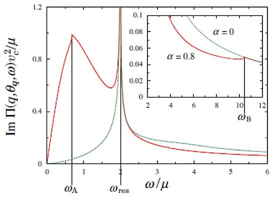
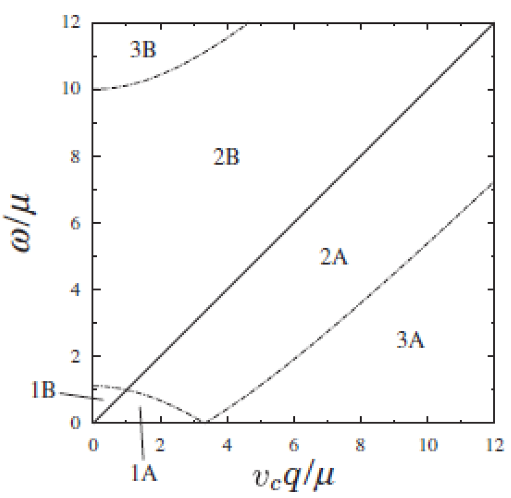
Figure 1.
Several regions on the q-ω plane for calculating the polarization function (Equation (3)). From [
23]. Reproduced with permission from JPSJ.
Figure 1.
Several regions on the q-ω plane for calculating the polarization function (Equation (3)). From [
23]. Reproduced with permission from JPSJ.
The results consist of six regions. These regions 1A, 2A, 3A, 1B, 2B, and 3B are classified into two regions, A and B, corresponding to the process of intraband and interband excitations, respectively. The regions A and B are separated by a solid line expressed as ω
res = (1 + cosθ
q)v
cq, which is called the resonance frequency. The resonance frequency is obtained owing to the nesting of the excitations with the linear dispersion, and the polarization function diverges with the chirality factor
Fs(
k). The boundary between 2A and 3A is given by ω
+. The boundary between 2A and 1A (2B and 1B) is given by ω
A. The boundary between 2B and 3B is given by ω
B. In the case of the isotropic Dirac cone (
i.e., α = 0), there is a boundary given by ω/μ + v
cq/μ = 2 which separates 1A and 2A (1B and 2B) for the intraband (the interband). In the regions 3A and 1B, the imaginary part vanishes. For the tilted Dirac cone, the boundary between 1A and 2A exhibits a noticeable behavior characterized by the appearance of cusps for the imaginary part as shown in
Figure 2.
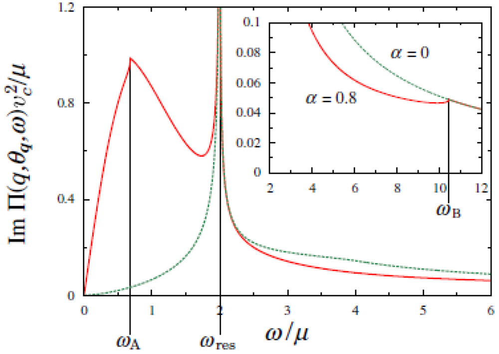
Figure 2.
Normalized imaginary part, Im Π(q,θq,ω) vc2/μ, as a function of ω/μ, for θq = π/2 and α = 0.8. From [
23]. Reproduced with permission from JPSJ.
Figure 2.
Normalized imaginary part, Im Π(q,θq,ω) vc2/μ, as a function of ω/μ, for θq = π/2 and α = 0.8. From [
23]. Reproduced with permission from JPSJ.
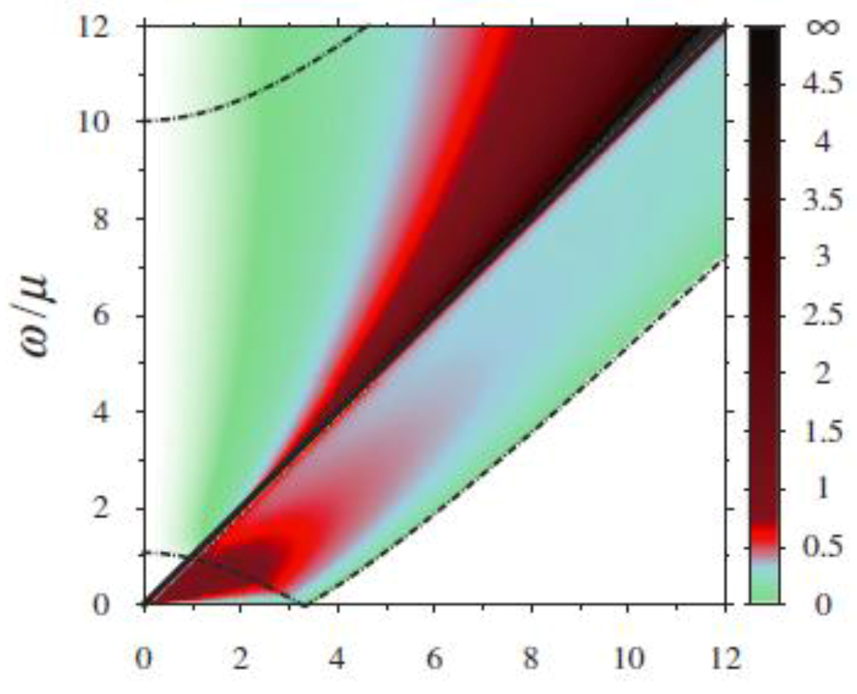
Figure 3 shows the normalized imaginary part, Im Π(θ
q,ω) v
c2/μ, on the plane of v
cq/μ and ω/μ for θ
q = π/2. The color gauge with the gradation represents the magnitude of the imaginary part. The global feature is mainly determined by the property of ω
res. In the case of v
c q/μ >> 1, where the characteristic energy becomes much larger than the interband energy, Im Π(θ
q,ω) of the intraband excitation (ω < ω
res) becomes much smaller than that of the interband excitation (ω > ω
res) in contrast to the case,v
c q/μ = 2. The broad peak in the intraband excitation does not change much for θ
q < π/2, while it is strongly masked for π/2 < θ
q < π due to the rapid decreasing ω
res.
Figure 3.
Normalized imaginary part, Im Π(θq,ω) vc2/μ, on the plane of vcq/μ and ω/μ for θq = π/2. From [
23]. Reproduced with permission from JPSJ.
Figure 3.
Normalized imaginary part, Im Π(θq,ω) vc2/μ, on the plane of vcq/μ and ω/μ for θq = π/2. From [
23]. Reproduced with permission from JPSJ.
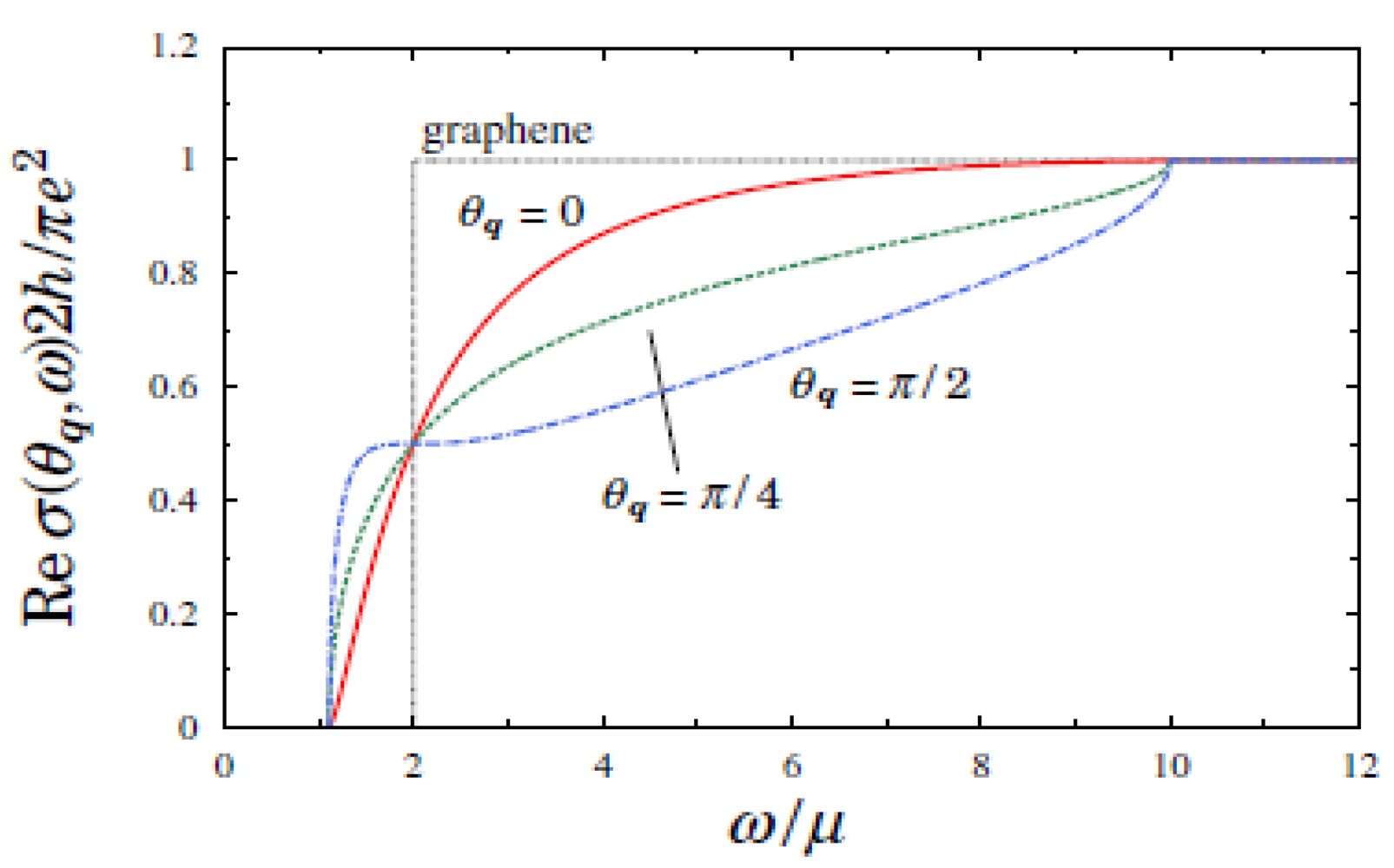
In
Figure 4 the normalized optical conductivity of Reσ(θ
q,ω) is shown as a function of ω/μ with some choices of θ
q = 0, π/4 and π/2, with α = 0.8. The dotted line denotes the isotropic case where Re σ is zero for ω < μ and is constant for μ < ω. The conductivity Re σ is zero for ω < 2 μ/(1 + α) and 1 for ω > 2μ /(1 – α), while it takes an intermediate value for 2 μ/(1 + α) < ω < 2μ/(1 – α).
Figure 4.
Normalized optical conductivity of Reσ(θ
q,ω) as a function of ω/μ. From [
23]. Reproduced with permission from JPSJ.
Figure 4.
Normalized optical conductivity of Reσ(θ
q,ω) as a function of ω/μ. From [
23]. Reproduced with permission from JPSJ.
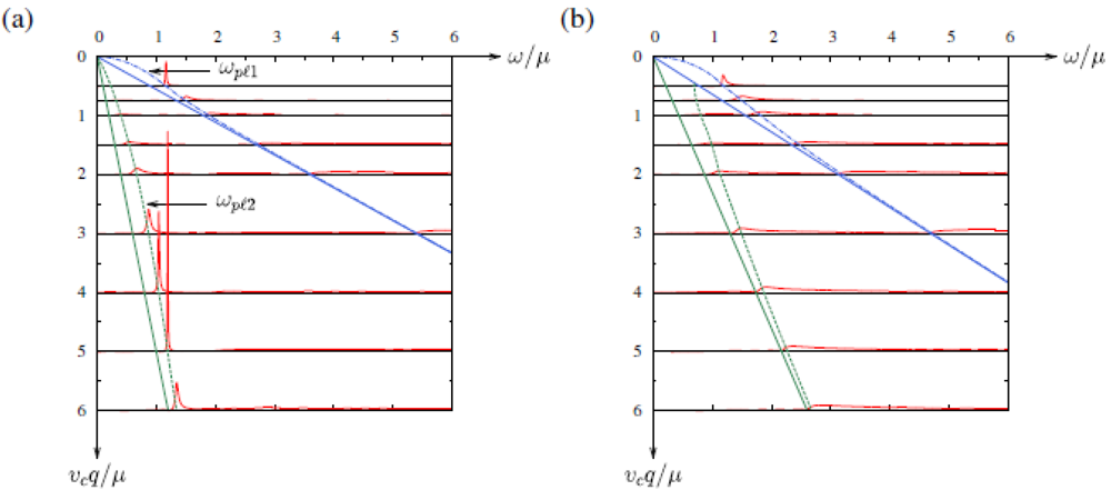
The plasma mode is calculated from 1 + vq ReΠ(q,θq,ωpl(1,2)) = 0 with vq = 2πe2/ε0q. Since the plasma frequency ωpl is located just above the resonance frequency, the solution is expected close to ωpl1 =ω0pl1 and ωpl2=ω0pl2, respectively. However, the imaginary part is complicated due to the combined effects of Π R(q,θq,ω) + Π L(q,θq,ω). We use the scaled quantities as qvc/μ and ω/μ with e2/(ε0vc) = 1. The plasma frequency corresponds to ω, which gives a peak of ImΠRPA(q,θq,ω).
In
Figure 5(a), Im Π
RPA(q,θ
q,ω) for θ
q = 0 is shown as a function of ω/μwith fixed v
cq/μ = 0.5, 0.75, 1, 1.5, 2, 3, 4, 5 and 6, respectively. The dash-dotted line (ω
pl1(q,θ
q) denotes the location of ω/μ for the peak of the plasmon, which is appreciable for small v
cq/μ. The dotted line denotes the location of ω for the novel plasmon,
i.e., ω
pl2(q,θ
q), which is found for the intermediate magnitude of v
cq/μ. Such a plasmon, ω
pl2(q,θ
q) originates from the interplay of two tilted cones. These two plasmons, which are found just above ω
res are obtained as the hybridization of the electron of the right cone and that of the left cone. The appreciable peak of Im Π
RPA(q,θ
q,ω) moves from ω
pl1(q,θ
q) to ω
pl2(q,θ
q) with increasing q,
i.e., the weight for small q is determined by ω
pl1(q,θ
q) and that of intermediate q is determined by ω
pl2(q,θ
q). In
Figure 5(b), Im Π
RPA(q,θ
q,ω) is shown for θ
q = π/4. It is found that the weight for ω
pl2(q,θ
q) is suppressed. This implies that both the dispersion relation and the intensity exhibit appreciable θ
q dependence. Such an anisotropy of the intensity gives rise to plasmon filtering. The novel plasmon has the following characteristics. The plasma frequency ω
pl2(q,θ
q) in the case of θ
q = 0 exists for any q. At θ
q = π/4, ω
pl2(q,θ
q) does not exist for small q, and is also absent for any q when θ
q = π/2. Furthermore, we find that ω
pl1(q,θ
q) is proportional to q
1/2 for small q, and that ω
pl2(q,θ
q)-ω
res is proportional to q for intermediate v
cq/μ.
Figure 5.
Im ΠRPA(q,θq,ω) as a function of ω/μwith fixed vcq/μ = 0.5, 0.75, 1, 1.5, 2, 3, 4, 5 and 6, for θq = 0 (a), and θq =π /4 (b). From [
24]. Reproduced with permission from JPSJ.
Figure 5.
Im ΠRPA(q,θq,ω) as a function of ω/μwith fixed vcq/μ = 0.5, 0.75, 1, 1.5, 2, 3, 4, 5 and 6, for θq = 0 (a), and θq =π /4 (b). From [
24]. Reproduced with permission from JPSJ.
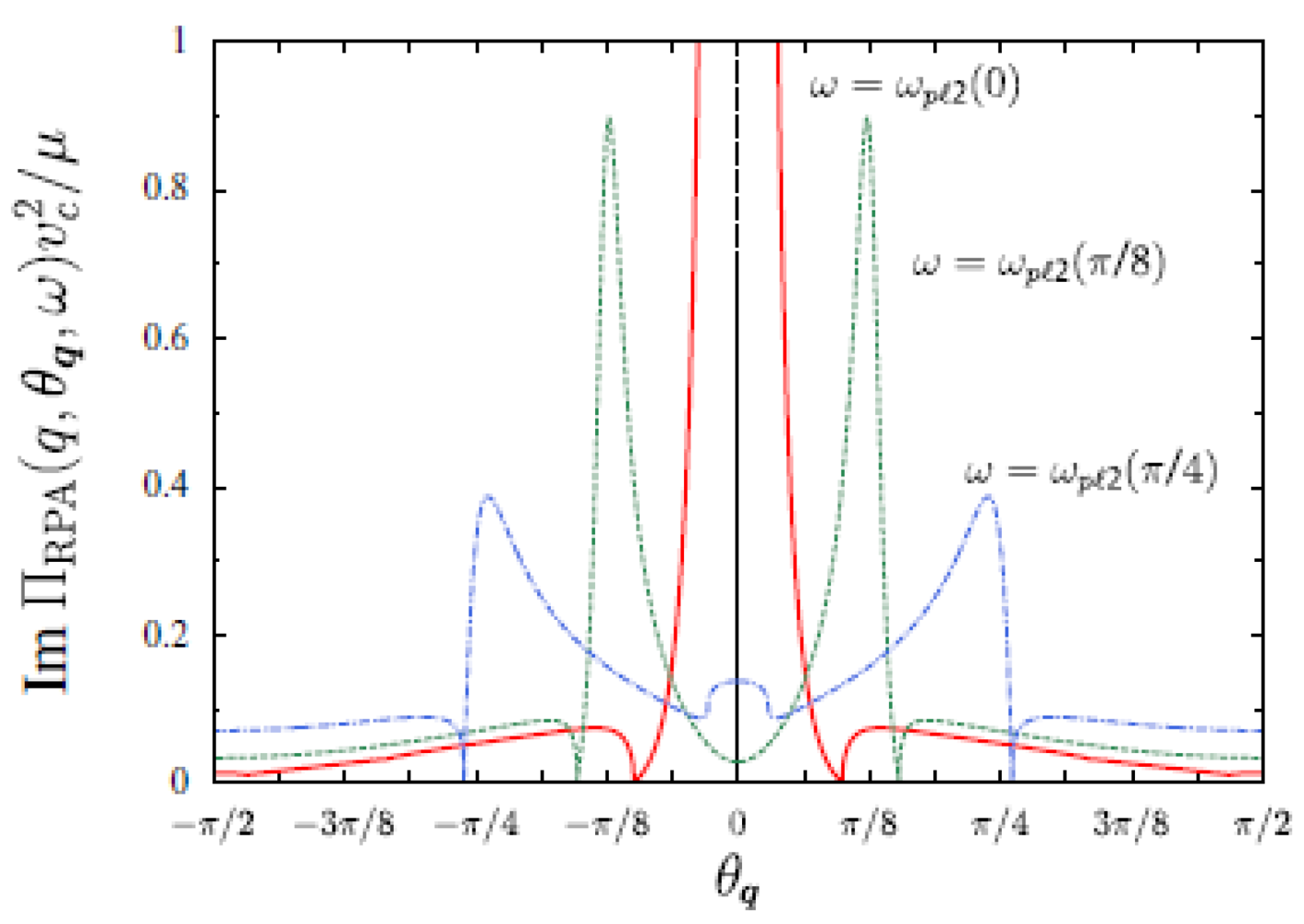
Here we examine the filtering of the plasma frequency by tuning the angle θ
q of the external field with frequency ω and q.
Figure 6 is an example of Im Π
RPA(q,θ
q,ω) when the external frequency is chosen as ω = ω
pl2(q,0) (solid line), ω
pl2(q,π/8) (dotted line), and ω
pl2(q,π/4) (dashed line) for the fixed v
cq/μ = 5. For ω = ω
pl2(q,0), a pronounced peak with the peak height (about 15) and the width (0.036 π) shows that the plasmon excitation occurs in the narrow region close to θ
q = 0. For the choice of ω = ω
pl2(q,π/8), the peak appears at θ
q = +(–)π/8 where the intensity is reduced less than 1/10 compared with ω = ω
pl2(q,0). The peak is further reduced for ω = ω
pl2(q,π/4). No peak is expected when the frequency is outside of the regime of the plasma frequency. In terms of the dielectric function ε(q,θ
q,ω), the location of the peak is determined by Reε(q,θ
q,ω) = 0 while the height and the width are determined by Im ε(q,θ
q,ω).Thus the peak (or the double peak) structure gives the filtering of plasmon, which depends on θ
q.
Figure 6.
θ
q dependence of Im Π
RPA(q,θ
q,ω) for v
cq/μ = 5 with the fixed ω = ω
pl2(q,0) (solid line), ω
pl2(q,π/8) (dotted line), and ω
pl2(q,π/4) (dashed line). From [
24]. Reproduced with permission from JPSJ.
Figure 6.
θ
q dependence of Im Π
RPA(q,θ
q,ω) for v
cq/μ = 5 with the fixed ω = ω
pl2(q,0) (solid line), ω
pl2(q,π/8) (dotted line), and ω
pl2(q,π/4) (dashed line). From [
24]. Reproduced with permission from JPSJ.
3. Berry Curvature of the Dirac Particle of α-(BEDT-TTF)2I3
The contact point in a normal state, i.e., without charge ordering, is determined essentially by the property of the transfer energy, and the effect of interaction is to modify mainly the location of the contact point. Then, by taking account of only the transfer energy, we examine the Hamiltonian for α-(BEDT-TTF)2I3 given by
where α and β(=1, 2, 3,4) are indices for the site of each molecule A(1), A'(2), B(3) and C(4) in the unit cell, and i, j are those for the cell forming a square lattice with N sites. The quantity
a denotes the annihilation operator for the electron, and
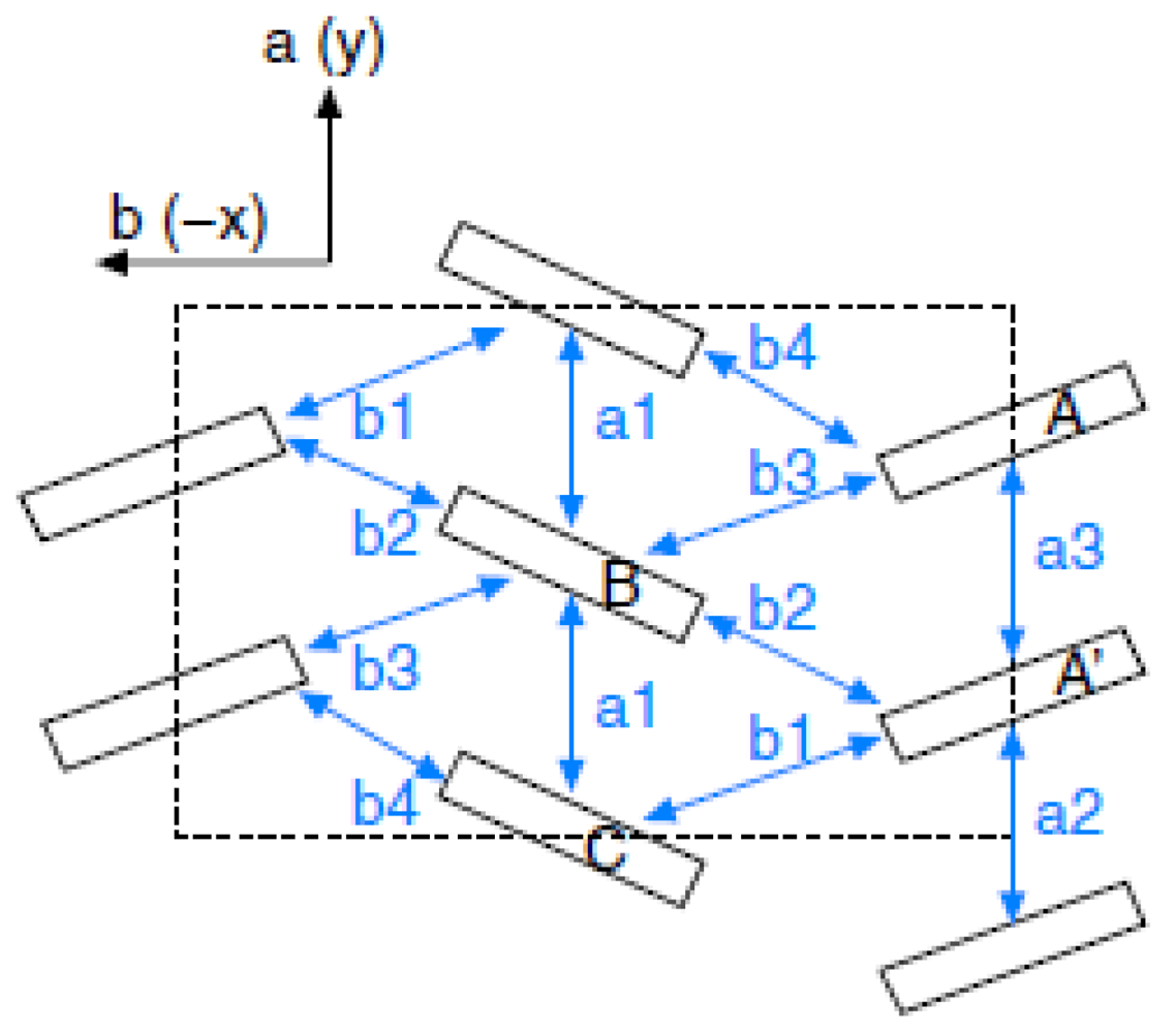
t denotes the transfer energy between the neighboring site. As shown in
Figure 7, there are seven transfer energies given by t
b1, …, t
b4 for the direction of the b(-x)-axis and t
a1, …, t
a3 for the direction of the a(y) -axis, respectively.
Figure 7.
Crystal structure on a two-dimensional plane with four molecules A(1), A’(2), B(3), and C(4), in the unit cell where the respective bonds represent seven transfer energies tb1, ..., ta3. From [
25]. Reproduced with permission from JPSJ.
Figure 7.
Crystal structure on a two-dimensional plane with four molecules A(1), A’(2), B(3), and C(4), in the unit cell where the respective bonds represent seven transfer energies tb1, ..., ta3. From [
25]. Reproduced with permission from JPSJ.
By introducing site potentials given by I1σ = −I2σ= −∆0, and I3σ = −I4σ = 0, the 4 × 4 Hamiltonian on the site basis and with a Fourier transform is given by
In the above Hamiltonian, kx is replaced by kx + π and then the center corresponds to X point. We obtain four bands Ej(k) where E1 > E2 > E3 > E4. For ∆0 = 0, the inversion symmetry between A and A' is kept, and E1 and E2 touches at Dirac point, k0, where the ZGS is found for the uniaxial pressure Pa being larger than 3 kbar. For the calculation of the Berry curvature, we consider the case of a finite value of ∆0, which induces a gap at the Dirac point.
The Berry curvature
Bn(
k) for each band E
n(
k) is calculated as [
29]
where |n > denotes the eigen vector of En. Note that B1(k) is essentially determined by E1 and E2, i.e., the effect of E3 and E4 is negligibly small within our numerical calculation. We define Bn(k) as the component of Bn(k), which is perpendicular to the kx − ky plane. For the small limit of ∆0, we obtain B1 = ∝ (∆0)−2.
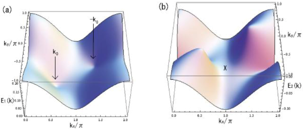
The energy band and Berry phase under uniaxial P
a are calculated using an extrapolation for
t (P
a) [
8]. Energy bands of E
1(a) and E
2(b) for Pa =6 kbar and ∆
0 = 0.02 eV is shown in
Figure 8(a) and (b).
Figure 8.
Energy bands of E1(a) and E2(b) for Pa = 6 kbar. From [
25]. Reproduced with permission from JPSJ.
Figure 8.
Energy bands of E1(a) and E2(b) for Pa = 6 kbar. From [
25]. Reproduced with permission from JPSJ.
The Dirac cone exists at +(-)k0, with k0= (0.57 π, - 0.3 π), as shown by arrows. A pair of cones is seen close to E1(k0) and E2(k0) and the cones in the same band are symmetric with respect to the Γ (=(0,0)) point. For E1(k), the maximum is seen at the Y(=(0,π)) point, while saddle points are seen for the X(=(0,π)), M(=(π,π)), and Γ points. For E2(k), the minimum is seen at the M point while saddle points are seen for the X, Y, and Γpoints. The accidental degeneracy, which is found at +(–)k0 for −△0 ➝ 0 is realized as the minimum of E1(k) and the maximum of E2(k).
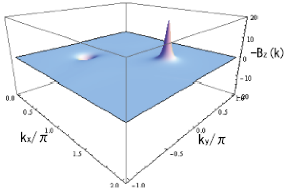
The corresponding Berry curvature B
1(
k) is shown in
Figure 9. The peak around –
k0 (+
k0) is positive (negative). They are antisymmetric with respect to the Γ. Since the curvature exhibits a noticeable peak close to +(–)
k0, such a peak may be identified as the Dirac particle instead of calculating the contact point.
Figure 9.
Berry curvature B
1(
k) (component perpendicular to the k
x–k
y plane). From [
25]. Reproduced with permission from JPSJ.
Figure 9.
Berry curvature B
1(
k) (component perpendicular to the k
x–k
y plane). From [
25]. Reproduced with permission from JPSJ.
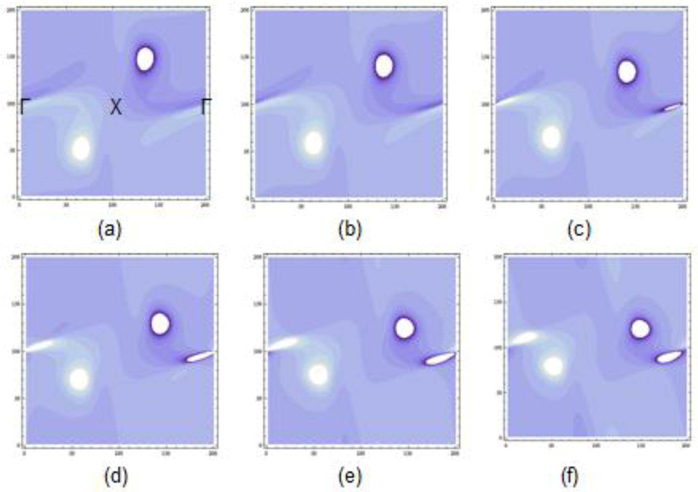
We examined the Berry curvature for other bands. The Berry curvature of the second band E
2(
k) is shown for several choices of P
a in
Figure 10. The peak located at +(–)
k0 has a sign opposite to that of E
1(
k).
Figure 10(d) denotes B
1(
k) at Pa = 6 kbar corresponding to
Figure 9. In addition to such a peak, another pair of peaks appears close to the Γ point. The latter one is rather extended to a direction slightly declined toward the horizontal axis, suggesting a large anisotropy of the Dirac cone. The anisotropic peak disappears for P
a smaller than 3 kbar while it becomes rather isotropic for large P
a. Such a behavior resembles the emergence of the Dirac particle in the charge ordered state, which has been shown in α-(BEDT-TTF)
2I
3 [
27]. The Berry curvature for E
3(
k) is obtained similarly where a pair of peaks close to the Γ point also exists with a sign opposite to that of E
2(
k). There is another peak close to the M point, which compensates for that of E
4(
k). These results show that each neighboring band provides a pair of Dirac particles followed by the Berry curvature with an opposite sign. When a pair of Dirac particles between neighboring two bands is found, one may expect a pair of Dirac particles for the other neighboring bands.
Figure 10.
Contour of the Berry curvature, B1(k), of the second band E2(k) for Pa = 0(a), 2(b), 4(c), 6(d), 8(e), and 10(f) kbar respectively. Γ = (0,0). The Dirac particle at k0 with the positive B1(k) exists in the bright region of kx > 0 and ky < 0.
Figure 10.
Contour of the Berry curvature, B1(k), of the second band E2(k) for Pa = 0(a), 2(b), 4(c), 6(d), 8(e), and 10(f) kbar respectively. Γ = (0,0). The Dirac particle at k0 with the positive B1(k) exists in the bright region of kx > 0 and ky < 0.
4. Zero-Gap State in α-(BEDT-TTF)2 NH4Hg(SCN)4
In addition to α-(BEDT-TTF)
2I
3, the ZGS, where a contact point of the Dirac cone coincides with the chemical potential, is predicted for α-(BEDT-TTF)
2 NH
4Hg(SCN)
4 under uniaxial pressure, P
c along the stacking axis [
26].
There are the electron and hole surfaces owing to band-overlap at ambient pressure. The ZGS emerges under the uniaxial pressure along the stacking axis in the conducting plane, for P
c > 5 kbar.
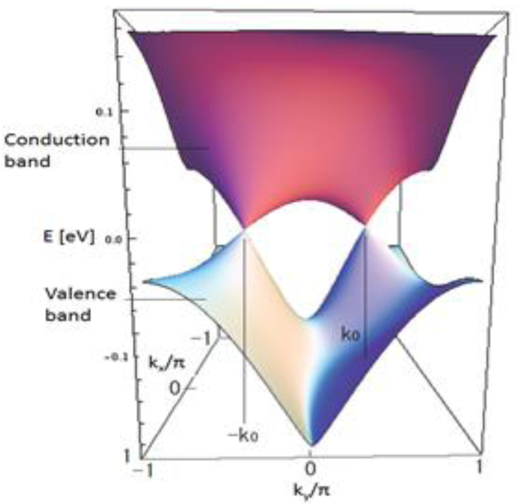
Figure 11 shows the energy dispersions of the conduction and valence band at P
c = 6 kbar, where the transfer energies are calculated by extrapolation using the data at P
c = 0 kbar [
30,
31] and 1.5 kbar [
31] obtained from the X-ray experiment
. A pair of the Dirac cones is located at k
0 = (−0.25, 0.51) π. The chemical potential coincides with the contact points since there is no band-overlap. The Dirac cones are rather isotropic compared with those of α-(BEDT-TTF)
2I
3.
The singularity of phase of the wave function, which describes the intrinsic property of the Dirac electron, has been confirmed using the Berry curvature. There is a pair of peaks in the Berry curvature, which corresponds to a pair of Dirac electrons with opposite chirality. The peaks of the Berry curvature are highly anisotropic at ambient pressure, while those become nearly isotropic at Pc = 6 kbar.
In addition, the effective Hamiltonian on the Luttinger-Kohn representation has been investigated. It has been found that the Dirac cone, which exists below the chemical potential, is anisotropic and tilted at ambient pressure. The anisotropy of the Dirac electron at ambient pressure is related to the one-dimension-like valley (ridge) structure between two contact points in the conduction (valence) band. The anisotropy and tilting of the Dirac cone are reduced with increasing pressure.
Figure 11.
Energy dispersions of the conductionand valence band at P
c = 6 kbar of α-(BEDT-TTF)
2 NH
4Hg(SCN)
4. From [
26]. Reproduced with permission from JPSJ.
Figure 11.
Energy dispersions of the conductionand valence band at P
c = 6 kbar of α-(BEDT-TTF)
2 NH
4Hg(SCN)
4. From [
26]. Reproduced with permission from JPSJ.
5. Emergence of Dirac Electron Pair in Charge Ordered State of α-(BEDT-TTF)2I3
We re-examined the band structure of the stripe charge ordered state of α-(BEDT-TTF)
2I
3 under pressure using an extended Hubbard model [
27]. The model used to describe the two-dimensional electronic system in α-(BEDT-TTF)
2I
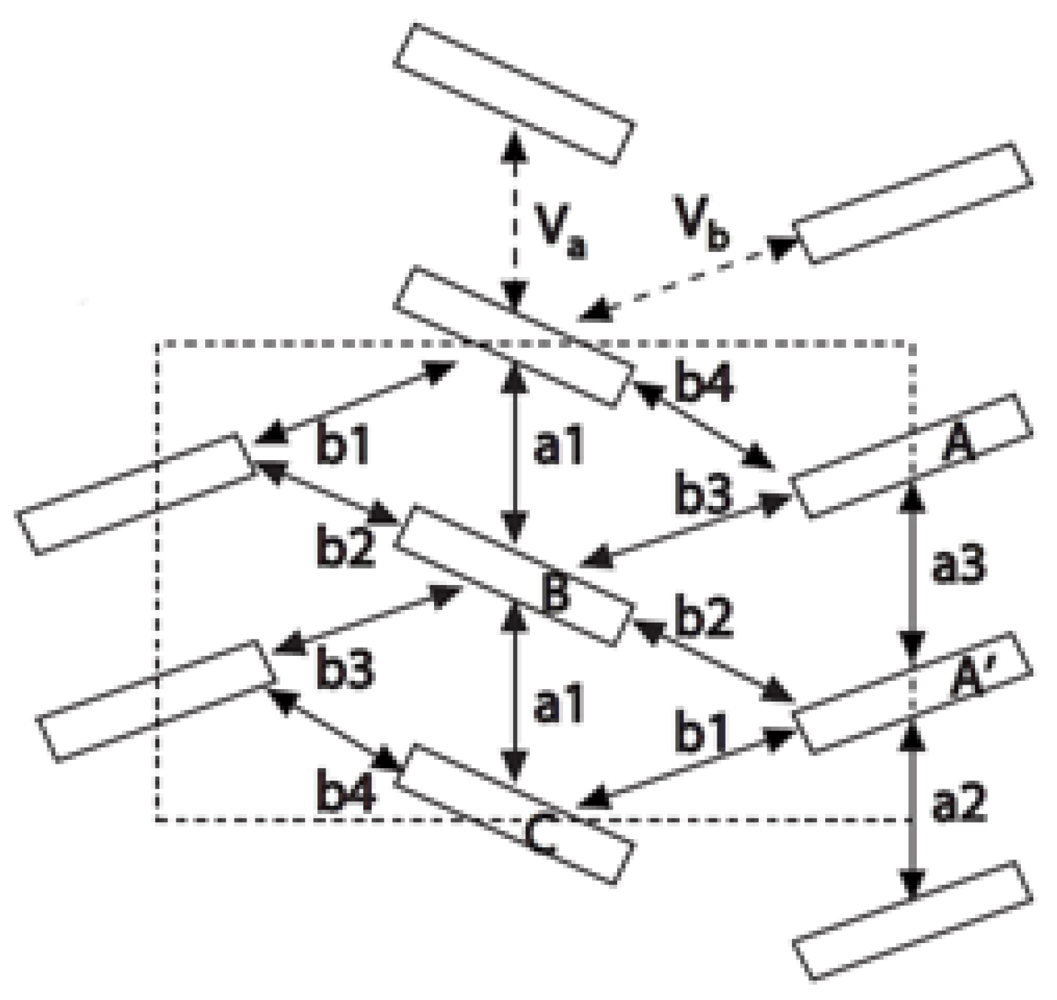
3 is shown in
Figure 12. The unit cell consists of four BEDT-TTF molecules on sites A, A’, B and C. The sites A, B and C are inequivalent, while A is equivalent to A’ so that inversion symmetry is preserved in the normal state. There are six electrons for the four molecules in a unit cell,
i.e., the band is 3
/4-filled. On the basis of the HOMO orbitals, the electronic system is described by the extended Hubbard model with several transfer energies, the on-site repulsive interaction
U and the anisotropic nearest-neighbor repulsive interaction
Vαβ,where i, j denote site indices of a given unit cell, and a,b = A, A’, B and C are indices of BEDT-TTF sites in the unit cell. In the first term, the transfer energies as a function of a uniaxial pressure (
Pa) along the
a-axis are estimated from an extrapolation using the data at P = 0 kbar [
2] and P
a = 2 kbar [
6]. We use the parameter
U = 0
.4 eV and the
Vab takes on two different values,
Va = 0.17~0
.18 eV along the stacking direction, and
Vb= 0
.05 eV along the perpendicular direction. With this choice of parameters, we obtain a pressure dependence of the electronic spectrum consistent with experimental results [
5]. Throughout the paper, the lattice constant is taken as unity. As in previous work [
32], we restrict ourselves to a Hartree mean field theory.
Figure 12.
The model describing the electronic system ofα-(BEDT-TTF)
2I
3. The unit cellconsists of four BEDT-TTF molecules A, A’, B and C with seven transfer energies. The nearestneighbor repulsive interactions are given by Vaand Vb [
27].
Figure 12.
The model describing the electronic system ofα-(BEDT-TTF)
2I
3. The unit cellconsists of four BEDT-TTF molecules A, A’, B and C with seven transfer energies. The nearestneighbor repulsive interactions are given by Vaand Vb [
27].
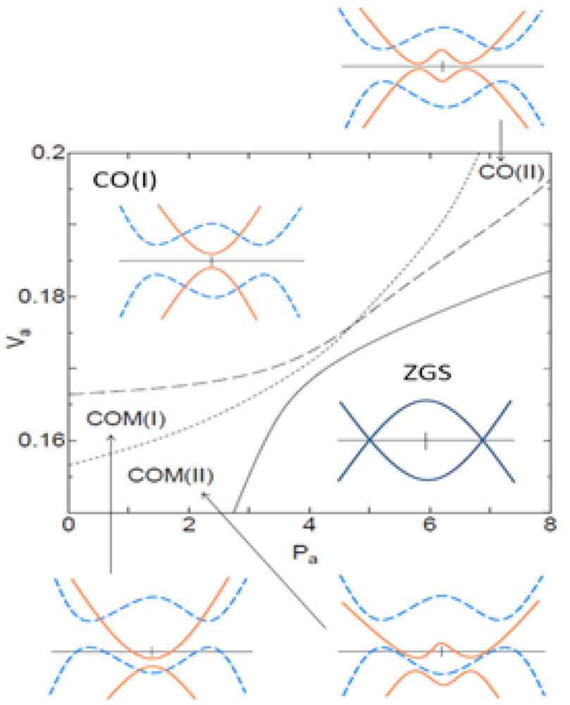
The
Pa-
Va phase diagram obtained from the self-consistent Hartree approximation is shown in
Figure 13 [
27]. This figure exhibits three transition lines. Two of them (the continuous and dashed lines) have already been found in previous work [
32] and the third one (dotted line) is a novel transition. The schematic band spectrum close to the Fermi surface is also shown in
Figure 13. The solid line marks a charge ordering transition resulting from the simultaneous breaking of time reversal and inversion symmetries. It separates the charge ordered metallic state (COM) from the Zero Gap state (ZGS). In the ZGS phase, energy bands are spin degenerate and inversion symmetry is preserved. Coming from this high-pressure ZGS phase and traversing the continuous line, the inversion symmetry is spontaneously broken by the electronic interactions. As a consequence, a gap opens leading to an insulating phase. However the time reversal symmetry is also spontaneously broken by the interactions so that the degeneracy between up and down bands is now lifted. Therefore the
simultaneous breaking of time reversal and inversion symmetries results in a semi-metallic phase (COM) with band overlap leading to small electrons and hole pockets of opposite spin orientations. In striking contrast with the continuous line, the dashed line marks a metal-insulator transition from a charge ordered metallic (COM) phase to a charge ordered insulator (CO) without breaking of any symmetry.
In traversing this transition line, the dispersion relations stay similar but their relative positions to the Fermi level vary. In this work, by a more detailed analysis of the COM and CO phases, we find a new
topological transition (dotted line in
Figure 13) that further splits each of the COM and CO phases into two phases: COM(I,II) and CO(I,II). This transition concerns a modification in the two energy bands close to the Fermi energy. They correspond to a given value of the spin that we choose to denote as “up”. The two other bands (down) are not concerned by this transition. As illustrated in
Figure 13, the transition from CO(I) to CO(II) is characterized by a change in the form of the dispersion relation of the valence and conduction bands. In the CO(I) phase, there is a single minimum of charge gap whose position in the k space stays at the M-point. In the CO(II) phase, the single charge gap separates into two points at symmetrical positions from the M-point. There is now a double-well structure in the dispersion relation. This transition corresponds to the emergence of a pair of Dirac points.
Figure 13.
The phase diagram on the
Pa-
Va plane, where
U = 0.4 eV, and
Vb = 0.05 eV [
27].The CO and COM denote insulating and metallic states with charge ordering ,respectively. Phase (I) shows a single minimum, while phase (II) is characterized by a doubleminimum in the up spin band. In the schematic energy spectrum close to the Fermi energy (horizontal line), thered and blue bands correspond to the up and down spin band, respectively.
This modification of the band structure is described by an effective low energy Luttinger-Kohn Hamiltonian with nine parameters that can be extracted from a numerical Hartree calculation. From a detailed study of this Hamiltonian and the corresponding energy spectrum, we show that the transition is driven by a single quantity det
SM whose sign changes at the transition.
SM is the stability matrix, which governs the stability of the M-point [
27]. A similar scenario occurs for the COM(I)-COM(II) transition.
The existence of a pair of Dirac points is characterized by a special structure of the Berry curvature. In the CO(II) and COM(II) states, the Berry curvature shows two sharp peaks with opposite signs. On the other hand, in CO(I) and COM(I) phases, the Berry curvature becomes very small owing to cancelation of the positive and negative contributions. The existence of the Dirac point is also verified by integrating the Berry curvature over a region limited by a closed energy contour around a single point [
27].
This topological transition could be probed in a magnetic field by the modification of the Landau level structure, therefore by e.g. magnetoresistance experiments.
6. Tilted-Cone-Induced Easy-Plane Pseudo-Spin Ferromagnet and Kosterlitz-Thouless Transition in Massless Dirac Fermions
We have considered the low-energy effective Hamiltonian for
N = 0 Landau states in a pair of tilted Dirac cones [
28] using the bases of the Wannier functions [
33] for the magnetic rectangular lattice, which is constructed by a linear combination of the wave functions of
N = 0 Landau states in the Landau gauge. This Wannier functions satisfy orthonormality and are localized around
R = (ma, nb) with integers
m and
n. A unit cell satisfies
ab = 2πl2 with the magnetic length
l = (hc/2π eH)1/2and has a magnetic flux quantum
hc/e. By taking the long-range Coulomb interaction and the Zeeman energy
EZ, the low-energy effective Hamiltonian is given by
where i, j, k, and l denote the unit cells of the magnetic rectangular lattice at Ri, Rj, Rk, and Rl, respectively, σ denote the spin, τ denote the valley-pseudo-spin which represents the degree of freedom on a pair of Dirac cones, and ciστ+ (ciστ) is the creation (annihilation) operator on the bases of the Wannier functions. The forward-scattering term of the long-range Coulomb interaction, Vijkl, comes from the long wave length part. This term does not depend on the spin and valley-pseudo-spin, and then it does not break the SU(4) symmetry, neither in the spin subspace nor in that of the pseudo-spin. It has been found that the forward-scattering term is not affected by the tilting. On the other hand, the backscattering term of the long-range Coulomb interaction, Wijkl, which is the inter-valley scattering term exchanging large momentum 2k0 and breaks the SU(2) symmetry in the subspace of the valley-pseudo-spin, comes from the short wave length part. In the absence of tilting, as e.g., in graphene, the backscattering term vanishes. We found that the tilting is essential to have a non-zero backscattering term. The ratio between the forward and backscattering terms is given by Wijkl/Vijkl~α2αL/l, where α is the tilting parameter, αL is the real lattice constant. The backscattering term is proportional to αL, since the large momentum |2k0|~π/αL is exchanged. We note that the lattice constant of α-(BEDT-TTF)2I3, αL~1 nm, is much larger than that of graphene. Thus it is expected that the backscattering term plays an important role for electron-correlation effects in α-(BEDT-TTF)2I3. The typical value of the ratio Wijkl/Vijkl is approximately 0.07 for α-(BEDT-TTF)2I3 at H = 10 T using the tilting parameter α = 0.8.
In the absence of an explicit symmetry breaking, such as the Zeeman effect or the above-mentioned backscattering term, no particular spin or valley-pseudo-spin channel is selected, and one may even find an entangled spin-pseudo-spin ferromagnetic state at low temperature. The symmetry-breaking terms may, thus, be viewed as ones that choose a particular channel (spin or valley-pseudo-spin) and direction of a pre-existing ferromagnetic state by explicitly breaking the original SU(4) symmetry.
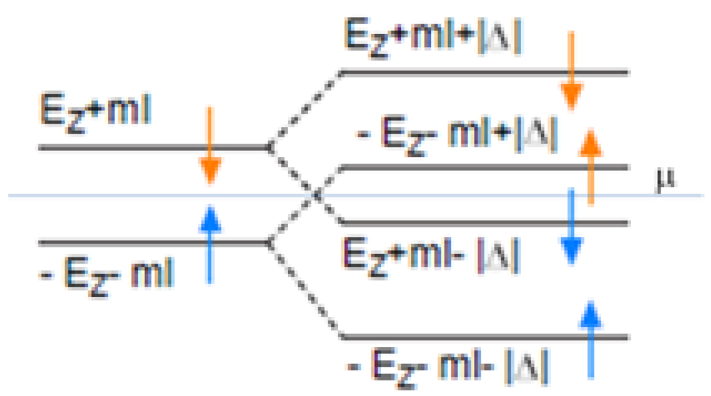
In the spin-polarized state without valley-pseudo-spin polarization (Δ = 0), electrons reside in the spin-up branches of the
N = 0 Landau levels as shown on the left hand side of
Figure 14, where
m is the spin polarization and
I is the on-site effective interaction in the magnetic rectangular lattice. In the valley-pseudo-spin ferromagnetic state, where the easy-plane (XY) pseudo-spin polarization lifts the valley-pseudo-spin degeneracy and then the spin polarization is suppressed as shown on the right hand side of
Figure 14. Although the mean field approximation gives the first order transition from the spin-polarized state to the valley-pseudo-spin-polarized state with decreasing temperature, the valley splitting of Landau levels owing to the partial valley-pseudo-spin polarization may occur continuously with decreasing temperature owing to the two-dimensional fluctuation. Actually, the valley-splitting has been observed in the interlayer magnetoresistance [
34].
Figure 14.
Schematic figure of the energy levels in the spin-polarized state (left hand side) and the valley-pseudo-spinferromagnetic state (right hand side). Blue and orange arrows denote the real spins, and μ is the chemical potential. From [
28]. Reproduced with permission from JPSJ.
Figure 14.
Schematic figure of the energy levels in the spin-polarized state (left hand side) and the valley-pseudo-spinferromagnetic state (right hand side). Blue and orange arrows denote the real spins, and μ is the chemical potential. From [
28]. Reproduced with permission from JPSJ.
In the presence of the order parameter with a finite amplitude, phase fluctuation exists with the characteristic length of spatial variation much longer than the fictitious lattice spacing. The effect of this phase fluctuation, which has so far been ignored in the mean-field approximation, is treated on the basis of the Wannier functions and the resulting model is similar to the XY model leading to the Kosterlitz-Thouless transition [
28].

