Abstract
In-cloud icing occurred on cables, wind turbines, and aircraft wings and may cause power transmission paralysis, energy dissipation, and unsafe flight. The study of atmospheric ice is crucial to facilitate the development of in-cloud icing prediction/detection and anti-/de-icing systems. Herein, atmospheric ice formed by high-wind-speed, in-cloud icing was obtained and reserved during icing tests in the 3 m × 2 m icing wind tunnel located at CARDC. Microstructures of atmospheric ice formed by high-wind-speed, in-cloud icing were observed and analysed using the microscopic observation method. A better description was established to explore the influence of the icing environment on ice microstructures, such as the size and shape of air bubbles and the boundaries of ice grains. Furthermore, an accurate density measurement was developed to allow a better practical density expression to consider the characteristics of the impacted surface and the effect of the flow field.
1. Introduction
Icing happens ubiquitously in nature or in industry. In most cases, especially when it occurs on lakes [1], sea lanes [2], coastal areas [3], aircraft wings [4], wind turbines [5], and transmission lines [6], icing is unexpected and might cause many inconveniences and even serious damage, such as structural failure, unsafe navigation, and deterioration of heat transfer in heat exchanger systems. Different from water-cooling icing, which is influenced by the heat conduction effect, in-cloud icing is a phenomenon where super-cooled water droplets impede, freeze, and accrete on the cold surface, which is a complex and unstable dynamic physical process. Ice formed by in-cloud icing is anisotropy due to the fluid-structure interaction in the accreting process and is closely related to the meteorological environment and characteristic parameters of the impacted surface, as shown in Figure 1.
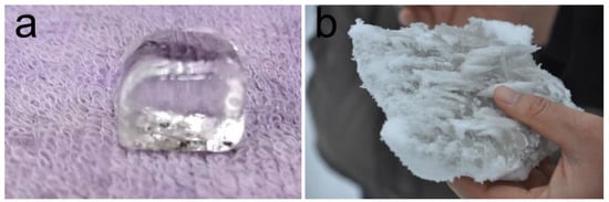
Figure 1.
Ices formed using different methods: (a) water-cooling icing; (b) in-cloud icing.
Similar to traditional crystal materials, such as metal, minerals, and ceramic, ice occurs as a polycrystalline polymer and the apparent performance is the sum of the individual grain’s behaviour [7,8,9]. As important as other crystalline materials, the macro-properties of ice are strongly dependent on its microstructures, which in return help to clarify the physical mechanism of the freezing process, establish the ice microstructure physical model under different conditions, and further the study the thermal, optical, electrical, and mechanical properties and behaviours of ice [10]. In recent years, researches focus on the microstructures of ice, and its physical properties have been rapidly developed due to their applications in many fields, for instance, cryo-sphere science, atmospheric science, geology and geophysics, ice engineering, aeronautical and astronautical science, technology, materials science, and so on [1,11,12,13]. With the constituent elements, the triggering, formation, development, and evolution of different ices were totally different and the basic structures of the interior ice were also varied, including texture (grain size, shape and orientation), crystalline, and impurities (such as air inclusions).
Currently, the research objects mainly focused on the ice formed by water cooling or originally from the precipitation of snow, for instance, seasonal lake (including reservoirs) ice [1], sea ice [14], and polar ice cores. Much progress has been made in exploring the microstructures, physical properties, and related engineering applications of the ice [15,16,17,18]. However, compared to ice which has abundant reserves and can be regularly sampled, atmospheric ice, usually assembled on aircraft wings, cables, and blades, is much more difficult to acquire and characterize. Moreover, there are still many difficulties in handling such a material which is easily broken and modified by a slight change in temperature [10]. Despite centuries of exploration, which has been focused on atmospheric ice, a detailed and in-depth understanding of ice microstructures is still lacking [19].
As a macroscopic representation of the microstructure of ice, density matters as same as the microstructure of aircraft icing. Analytical ice-accretion prediction codes, such as FENSAP-ICE and ICECREMO, used estimated ice density as an input parameter in performing the thickness of the accreted ice [20]. An improved description of microstructures with a better understanding of the effect of icing conditions on microstructures and densities would permit more accurate ice-accretion codes. In the past, an apparent density measurement of atmospheric ice was mainly performed by using a rotating multi-cylinder technique at low wind speeds. Ulteriorly, the density was evaluated and predicting the relationships for density was developed and modified by many researchers [21,22,23,24,25]. However, these practical expressions were established only considering a low-wind-speed (usually <40 m/s) icing environment with the limit of using a simple rotating cylinder as an impacted object, which is barely supported for an aircraft icing prediction/detection at high wind speeds.
Herein, based on a 3 m × 2 m ice wind tunnel located at the China Aerodynamics Research and Development Center (CARDC), this article presented and discussed the results of preliminary measurements of atmospheric ice obtained during high-wind-speed icing tests. Microstructures were observed and analysed at a given location inside a slice of ice. Apparent density measurements were performed using the drain away liquid method, which could extend the density measurement to non-rotating irregular bodies, such as airfoils at high wind speeds. Results for atmospheric ice were presented by taking into account the influence of high wind speeds. The improved understanding and characterisation of the microstructure and density of atmospheric ice would contribute to the aircraft icing prediction/detection system and anti-/de-icing system design.
2. Materials and Methods
2.1. Icing Wind Tunnel
The 3 m × 2 m icing wind tunnel is the biggest high-subsonic, close-loop refrigerated wind tunnel in the world with three changeable test sections located in CARDC, which contains a jet system, refrigeration system, height simulation system, and fan power system, as shown in Figure 2. In the most commonly used 3 m (width) × 2 m (height) × 6.5 m (length) test section, the total air temperature can be controlled from −40 °C to room temperature within ±0.5 °C. Velocities range from 21 m/s to 210 m/s and an estimated altitude of up to 20,000 m can be achieved. A spray system allows control of the liquid water content (LWC) ranging from 0.2 g/m3 to 3.0 g/m3. The spray nozzles provide a droplet median volume diameter (MVD) from 10 μm to 300 μm.
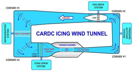
Figure 2.
3 m × 2 m icing wind tunnel.
2.2. Aircraft Atmospheric Ice Library
The aircraft atmospheric ice sample library was established when the 3 m × 2 m icing wind tunnel went into operation in 2013, and the icing conditions were chosen according to the FAA/FAR (Federal Aviation Administration Regulations) Appendix C, which summarized and provided the atmospheric icing conditions in real aeronautical meteorology. The ice samples, which were classified and stored in refrigeration maintained at −40 °C, originated from ice shapes accreted on airfoils from a variety of aircraft model icing tests, as shown in Figure 3. The ice samples were divided into two groups, one group was intensively sliced for microstructure observation, and the other group was measured for density measurement.
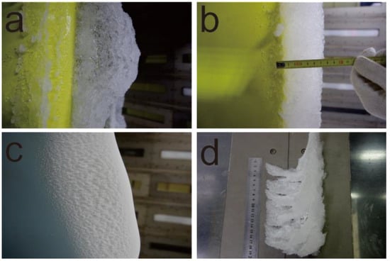
Figure 3.
Aircraft atmospheric ice library: (a–c) ices accreted on different airfoils; (d) processing and recording process before stored in the refrigerator.
2.3. Microstructure Measurement
The test specimens for the microstructure measurement and density measurement were prepared using the same ice sample, and the whole testing process was carried out in a cryogenic incubator, as shown in Figure 4. Firstly, the top and bottom surface of the ice sample was flatly sliced, and then the suitable-thickness ice sample was placed on a heated glass slide, of which the temperature was slightly higher than the ice’s freezing point. Thus, the bottom of the ice was slightly melted, and immediately refrozen and fixed to the surface of the glass slide in the cold environment for further observation. The microstructure of the ice slice was observed through an Olympus CX33 (Japan) optical microscope, with a 10× eyepiece and a 4× objective lens. The acquired image was 3072 × 2048 pixels, and each pixel was calibrated to 6.024 ×10⁻⁴ mm.
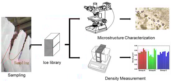
Figure 4.
Microstructure and density measurement of atmospheric ice.
2.4. Density Measurement
The density of the ice was carried out using an electronic liquid density instrument (MH-100E, Qunlong Tech, Shenzhen, China). The instrument was put in a cold environment for more than 8 h before the density measurement. The buoyancy of the ice was tested through drain-away liquid therapy, of which the liquid media was water-immiscible and had a low freezing point. The density of the irregular ice could be obtained using Equation (1):
where was the apparent density of the ice, and were the weight when the ice was in dry air and the weight when the ice was totally immersed into the liquid with the buoyancy created by the liquid, respectively, while was the known density of the liquid media.
3. Results and Discussion
3.1. Appearance
The ice samples far from the airfoil were selected to exclude the effect of the substrate influence on the ice microstructures. Figure 5 presented the microstructures of two typical atmospheric pieces of ice produced at different ambient tunnel temperatures at −5.8 °C and −25 °C, respectively. Beyond that, they were all produced at a moderate tunnel wind speed of 100 m/s, a similar MVD and LWC at about 20 μm and 0.5 g/m3. Differentially, their exterior appearances and internal structures were completed in an extreme variation. The two produced samples respectively had a transparent and a milky white appearance, which is called apparent ice and rime ice. The corresponding microstructures were discussed afterwards in detail, including grain size, bubble size, and bubble distribution.
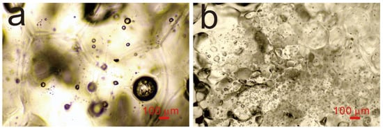
Figure 5.
Microstructures of different appearances of the atmospheric ices formed by the high-wind-speed in-cloud icing: (a) nearly transparent; (b) white appearance.
3.2. Grain Boundaries
The grain boundaries of the ice samples could be observed by the microscope images. The red dashed line highlighted the contours of the grain boundaries within the ice samples at the same LWC, speed, MVD, and altitude, but at different temperatures of −5.8 °C and −25 °C, as shown in Figure 6. The polycrystalline structure of the ice was clearly observed and stuck out by red dashed lines. The average sizes of the grains were approximately 500–800 μm and 100–200 μm for the nearly transparent ice and rime ice, respectively. It can be pointed out immediately that the grains were much larger in the apparent ice rather than the rime ice, which were coordinated well with the different freezing rates.
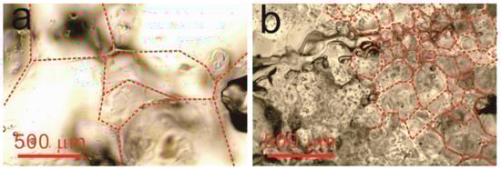
Figure 6.
Typical images and contours of the grain boundaries for atmospheric ice at different icing environments: (a) T= −5.8 °C, LWC = 0.5 g/m3, V = 100 m/s, MVD = 21.7 μm, Altitude = 3000 m; (b) T= −25 °C, LWC = 0.5 g/m3, V = 100 m/s, MVD = 21.2 μm, Altitude = 3000 m.
3.3. Air Bubbles
Different icing temperatures will directly lead to the difference in the grain size. Moreover, there were many bubbles that existed in the atmospheric ice. To further explore the effect of a single factor under different icing environments on the size and number of air bubbles or air inclusions, atmospheric ices formed by different icing environments were picked out. Figure 7 presented three different distributions of air bubbles at different temperatures as described. The ices were all produced at a relatively high tunnel wind speed of 100 m/s and a similar MVD and LWC. The detailed icing environment is listed below in Figure 7.
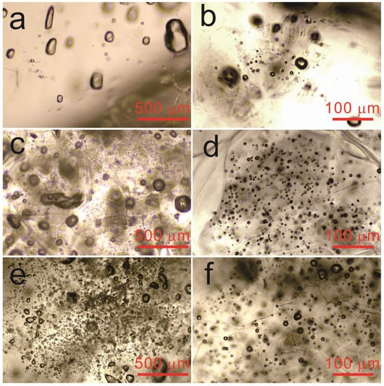
Figure 7.
Distribution of air bubbles of the high-wind-speed atmospheric ices obtained at different icing environments: (a,b) T= −5.8 °C, LWC = 0.5 g/m3, V = 100 m/s, MVD = 21.7 μm, Altitude = 3000 m; (c,d) T= −22 °C, LWC = 0.512 g/m3, V = 100 m/s, MVD = 20 μm, Altitude = 3000 m; (e,f) T= −25 °C, LWC = 0.5 g/m3, V = 100 m/s, MVD = 21.2 μm, Altitude = 3000 m.
In general, we distinguished the microscope-displayed bubble diameters into three categories: mini bubbles (diameters < MVD), microbubbles (MVD < diameters < 100 μm), and macro bubbles (diameters > 100 μm). The mini bubbles were common in every ice type and mainly distributed within the ice grain boundaries. When a super-cooled droplet impinged at the surface, due to the air dissolved in the water, the mini tiny weeny bubbles were precipitated and had no time to escape during the rapid ice crystal growth [12]. It was implied that the air solubility and rapid freezing rates were responsible for the formation of mini bubbles in the atmospheric ice. In addition, the microbubbles were responsible for the appearance and types of ice due to the light scatted and refracted in the bubbles with suited diameters [10]. As illustrated in Figure 7, the microbubbles conspicuously dominated the opaque appearance of the rime ice. Some researchers believed that the medium volume diameter (MVD) of the droplet was closely related to this kind of bubble, yet it still needs to be verified for the moment. It was not difficult to find out that as the temperature decreased, the number of mini and microbubbles increased. As displayed in Figure 7e,f, the circularity of the bubble, which was defined as the ratio of the long axis to the short axis, changed along with the decreased temperature.
More interestingly, the macro bubbles, more accurately referred to as air inclusions, usually exhibited irregular shapes and, especially, presented along the grain boundaries, which was in sharp contrast to the circular bubbles. This kind of bubble is strongly affected by the icing environment and dominated the porosity and density of the ice. While microbubbles were abundant in the ice, most of the air porosity resulted from the presence of macro bubbles. With the icing environment varied, the different types, quantities, and distribution of air bubbles would result in different porosity.
3.4. Porosity
The porosity of the atmospheric ice was calculated using two methods: microstructure characterisation and density comparison. Figure 8 illustrated the microstructure image processing results of the atmospheric ice under certain icing environments (T= −25 °C, LWC = 0.5 g/m3, V = 100 m/s, MVD = 21.2 μm, Altitude = 3000 m). Due to the gradient grey level, the observed air inclusion edges could be extracted with the aid of image analysis software (Imageview version 2018), in which the original picture was binarized. Afterwards, the statistical bubble size distribution was carried out under the assumption that the bubbles were perfect spheres. The software was programmed to automatically calculate and analyse parameters, such as the equivalent circular diameter, the area, and the distribution of the roughly circular air inclusions.
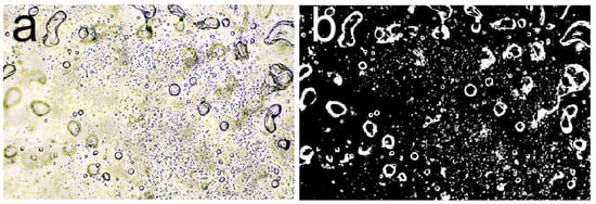
Figure 8.
Typical image and contours of the air inclusions for atmospheric ice produced at T= −25 °C, LWC = 0.5 g/m3, V = 100 m/s, MVD = 21.2 μm, Altitude = 3000 m. The porosity was calculated to be 7.88 % after image binarization, edge extraction, and the distribution statistical process: (a) image observed form microscope; (b) image after ImageView processing.
Since the air inclusions appeared only as two-dimensional projections in the images, the air volume fraction was approximated by the surface area fraction, which was originally acquired in 2D images as defined in Equation (2):
where N was the quantity of the bubbles and presented the area of a single bubble in the selected 2D image. was the sum of the area of each bubble and was the total area of the selected image.
Coincidentally, the porosity could also be predicted by comparing the true density and apparent density illustrated in Equation (3). The apparent density was obtained through the drain-away liquid therapy as described above, and the true density of pure ice was defined by Equation (4) [26].
For this ice sample, the porosity was calculated to be 7.88 % using microstructure characterisation, coordinated well with 7.61% obtained by density comparison.
3.5. Apparent Density
As a macroscopic representation of the microstructure of atmospheric ice, the density () information was required to have a better understanding of the ice microstructure. Since Macklin first calculated the atmospheric ice density by measuring the weight and volume of the ice accreted on the rotating cylinder, many researchers have developed and modified the practical expressions to construct the curves relating to (, as shown in Figure 9 [21,23,24,25], where was the impacting speed, was the effective median volume droplet diameter for each cylinder, and represented the surface temperature. However, unlike the ice accreted on the simple rotating cylinder, the volume of atmospheric ice obtained at the airfoil in our work could not be easily estimated due to the irregular shape, neither spanwise nor chordwise.
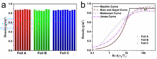
Figure 9.
(a) Measured density values of the atmospheric ice formed by high-wind-speed, in-cloud icing; (b) measured densities in this work fitted with previous density functions of R (Macklin Curve [21], Bain and Gayet Curve [23], Makkonen Curve [24], and Jones Curve [25]).
In our work, a density measurement of the atmospheric ice was carried out to eliminate the error caused by inaccurate volume, which was calculated by using a hand-painted icing area at the circular cross-section times the height of the cylinder. As listed in Table 1, three groups were classified as shown in Figure 9a. The density values of atmospheric ice we tested were related to R and ended up with a bunch of data points, likewise, as illustrated in Figure 9b. It was revealed that R was strongly affected by the wind speed, thus, the samples in our atmospheric ice library were all in the high value of R. The density functions of R, which were developed by data points from previous work, were in the range of low wind speeds (less than 40 m/s). Obviously, the lack of rigour is taking into account with the influence of the flow field and the characteristics of the impacted surface. Namely, the established relationship, which tended to be fixed as R, increased higher and could not be used to effectively explain the densities of atmospheric ice formed by high-wind-speed, in-cloud icing. Furthermore, the effect of the flow field and the characteristics of the impacted object should be taken into consideration. These suggested and required that we continue to investigate and carried out the accurate measurement of atmospheric ice densities to establish a better practical density predicting model.

Table 1.
Information on the high wind speed impacting ice at different icing environments.
Herein, referring to the transformation theory of the ice wind tunnel tests [27], has been proposed and defined in Equation (5), which is considered a reasonable combination of the parameters to define the effect of the characteristics of the impacted surface, the conserved momentum, and energy in the flow field and icing environment. In the equation, presented the freezing factor of impacting water on the surface, which was deduced from the energy conservation equation of the Messinger model [28]. was the droplet collection coefficient, which could be influenced by the droplet trajectories related to the flow field. LWC and were the liquid water content in and the flow velocity in , respectively.
Among them, was the latent heat of freezing and was the specific heat capacity of water on the model surface. In addition, three parameters were introduced to describe the process of heat balance: relative heat coefficient (), droplet energy transfer potential (), and air energy transfer potential ().
where was the surface temperature, was the static temperature, was the water film temperature, was the vapour pressure of water in the atmosphere, was the vapour pressure of water over liquid water, was the convective heat transfer coefficient, was the gas-phase mass transfer coefficient, and was the latent heat of evaporation.
was the droplet inertia coefficient and defined as follows [29]:
where was the average resistance ratio in connection with MVD, , and altitude, while was the uncorrected droplet inertia coefficient [30].
A curve relating to practice for impacting ice was estimated to better describe the relationship between the apparent densities and icing conditions as shown in Equation (12) and Figure 10.
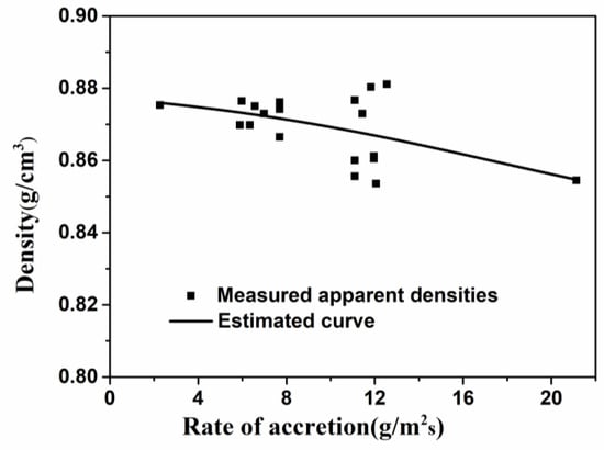
Figure 10.
Measured apparent densities and the estimated curve relating densities and ice accretion rates obtained by high-wind-speeds impacting ice.
The predictable densities obtained from this equation could effectively explain the effect of icing conditions on microstructures and densities of ice formed at high wind speeds, which were matched with the speed of an aircraft takeoff/landing, although the relationship needs to be further optimised due to the small amount of the acquisition data.
4. Conclusions
Herein, the low-temperature microscopy method that we developed allowed the observation of many features as the boundaries of ice grains, the size and shape of air bubbles, and promoted a better understanding of the formation and evolution of the microstructures for atmospheric ice formed by high-wind-speed, in-cloud icing. Furthermore, the accurate density measurement we developed could be used to measure the ice density formed on irregular bodies, such as airfoils. It has been demonstrated that the porosity calculated by microstructure characterisation coordinated well with the results estimated by the density measuring method, which verified the reliability of the measurement. Based on the selected ice samples from the aircraft atmospheric ice sample library, the densities were systematically investigated and demonstrated in the range of 0.85–0.89, which could not be accurately predicted by the existing empirical formulas, such as the Macklin Curve [21], the Bain and Gayet Curve [23], the Makkonen Curve [24], and Jones’ Curve [25]. Thus, the density prediction formula for atmospheric ice formed at high wind speeds was conducted using the icing rate (), which combined the characteristics of the impacted object and the effect of the flow field. The improved description and characterisation of microstructures and densities will facilitate a better understanding of atmospheric ice of the physical properties and pave the road to an in-cloud icing prediction/detection system and anti-/de-icing system design.
Author Contributions
Conceptualization, X.Y. and Q.W.; methodology, R.L.; investigation, R.L.; resources, X.Y.; data curation, Y.L.; writing—original draft preparation, R.L.; writing—review and editing, X.Y.; supervision, X.Y.; funding acquisition, X.Y. All authors have read and agreed to the published version of the manuscript.
Funding
This research was funded by KEY PROGRAMME OF NATIONAL NATURAL SCIENCE FOUNDATION OF CHINA, grant number 12132019.
Data Availability Statement
Data sharing is not applicable to this article.
Conflicts of Interest
The authors declare no conflict of interest.
References
- Huang, W.; Li, Z.; Han, H.; Niu, F.; Lin, Z.; Leppäranta, M. Structural analysis of thermokarst lake ice in Beiluhe Basin, Qinghai–Tibet Plateau. Cold Reg. Sci. Technol. 2012, 72, 33–42. [Google Scholar] [CrossRef]
- Lieb-Lappen, R.M.; Golden, E.J.; Obbard, R.W. Metrics for interpreting the microstructure of sea ice using X-ray micro-computed tomography. Cold Reg. Sci. Technol. 2017, 138, 24–35. [Google Scholar] [CrossRef]
- Timco, G.W.; Weeks, W.F. A review of the engineering properties of sea ice. Cold Reg. Sci. Technol. 2010, 60, 107–129. [Google Scholar] [CrossRef]
- Yamazaki, M.; Jemcov, A.; Sakaue, H. A Review on the Current Status of Icing Physics and Mitigation in Aviation. Aerospace 2021, 8, 188. [Google Scholar] [CrossRef]
- Wang, Q.; Yi, X.; Liu, Y.; Ren, J.; Li, W.; Wang, Q.; Lai, Q. Simulation and analysis of wind turbine ice accretion under yaw condition via an Improved Multi-Shot Icing Computational Model. Renew. Energy 2020, 162, 1854–1873. [Google Scholar] [CrossRef]
- Fan, C.; Jiang, X. Analysis of the Icing Accretion Performance of Conductors and Its Normalized Characterization Method of Icing Degree for Various Ice Types in Natural Environments. Energies 2018, 11, 2678. [Google Scholar] [CrossRef]
- Sammonds, P.; Montagnat, M.; Bons, P.; Schneebeli, M. Ice Microstructures and Microdynamics. Philos. Trans. A Math Phys. Eng. Sci. 2017, 375, 2086. [Google Scholar] [CrossRef]
- Parida, K.; Dehury, S.K.; Choudhary, R.N.P. Structural, Electrical and Magneto-Electric Characteristics of BiMgFeCeO6 Ceramics. Phys. Lett. A 2016, 380, 4083–4091. [Google Scholar] [CrossRef]
- Liu, L.; Chen, Y.; Feng, Z.; Wu, H.; Zhang, X. Crystal Structure, Infrared Spectra, and Microwave Dielectric Properties of the EuNbO4 Ceramic. Ceram. Int. 2021, 47, 4321–4326. [Google Scholar] [CrossRef]
- Pervier, M.A.; Pervier, H.; Hammond, D.W. Observation of microstructures of atmospheric ice using a new replica technique. Cold Reg. Sci. Technol. 2017, 140, 54–57. [Google Scholar] [CrossRef]
- Weeks, W.F.; Ackley, S.F. The Growth, Structure, and Properties of Sea Ice; Plenum Press: New York, NY, USA, 1986. [Google Scholar]
- Chu, F.; Zhang, X.; Li, S.; Jin, H.; Zhang, J.; Wu, X.; Wen, D. Bubble formation in freezing droplets. Phys. Rev. Fluids 2019, 4, 71601. [Google Scholar] [CrossRef]
- Blackford, J.R. Sintering and microstructure of ice: A review. J. Phys. D: Appl. Phys. 2007, 40, R355–R385. [Google Scholar] [CrossRef]
- Crabeck, O.; Galley, R.; Delille, B.; Else, B.; Geilfus, N.-X.; Lemes, M.; Des Roches, M.; Francus, P.; Tison, J.-L.; Rysgaard, S. Imaging air volume fraction in sea ice using non-destructive X-ray tomography. Cryosphere 2016, 10, 1125–1145. [Google Scholar] [CrossRef]
- Michel, B.; Ramseier, R.O. Classification of River and Lake Ice Based on Its Genesis, Structure and Texture; Laval University Press: Quebec City, QC, Canada, 1969. [Google Scholar]
- Gow, A.J.; Govoni, J.W. Ice Growth on Post Pond, 1973–1982; Cold Regions Research and Engineering Laboratory: Hanover, NH, USA, 1983. [Google Scholar]
- Michel, B.; Ramseier, R.O. Classification of river and lake ice. Can. Geotech. J. 1971, 8, 36–45. [Google Scholar] [CrossRef]
- Cherepanov, N. Classification of ice of natural water bodies. In Proceedings of the Ocean 74-IEEE International Conference on Engineering in the Ocean Environment, Halifax, NS, Canada, 21–23 August 1974; pp. 97–101. [Google Scholar]
- Farid, H.; Farzaneh, M.; Saeidi, A. A contribution to the study of the compressive behavior of atmospheric ice. Cold Reg. Sci. Technol. 2016, 121, 60–65. [Google Scholar] [CrossRef]
- Myers, T.G.; Charpin, J.P.F. A mathematical model for atmospheric ice accretion and water flow on a cold surface. Int. J. Heat Mass Transf. 2004, 47, 5483–5500. [Google Scholar] [CrossRef]
- Macklin, W.C. The density and structure of ice formed by accretion. Q. J. R. Meteorol. Soc. 1962, 88, 30–50. [Google Scholar] [CrossRef]
- List, R. The accretion of ice on rotating cylinders. Q. J. R. Meteorol. Soc. 1963, 89, 551–555. [Google Scholar] [CrossRef]
- Bain, M.; Gayet, J.F. Contribution to the modelling of the ice accretion process: Ice density variation with the impacted surface angle. Ann. Glaciol. 1983, 4, 19–23. [Google Scholar] [CrossRef]
- Makkonen, L.J.; Stallabrass, J.R. Ice Accretion on Cylinders and Wires; National Research Council Canada: Ottawa, ON, Canada, 1984. [Google Scholar]
- Jones, K.F. The density of natural ice accretions related to nondimensional icing parameters. Q. J. R. Meteorol. Soc. 1990, 116, 477–496. [Google Scholar] [CrossRef]
- Pounder, E.R. The Physics of Ice; Pergamon Press: Oxford, UK, 1965. [Google Scholar]
- Anderson, D.N. Manual of Scaling Methods; Ohio Aerospace Institute: Cleveland, OH, USA, 2004. [Google Scholar]
- Langmuir, I.; Blodgett, K. A Mathematical Investigation of Water Droplet Trajectories; Army Air Forces TR, USA No. 5418; 1946. [Google Scholar]
- Yi, X.; Zhu, G.; Wang, K.; Li, S. Numerically simulating of ice accretion on airfoil. Acta Aerodyn. Sin. 2002, 20, 428–433. [Google Scholar] [CrossRef]
- Bragg, M.B. A similarity analysis of the droplet trajectory equation. AIAA J. 1982, 20, 1681–1686. [Google Scholar] [CrossRef]
Disclaimer/Publisher’s Note: The statements, opinions and data contained in all publications are solely those of the individual author(s) and contributor(s) and not of MDPI and/or the editor(s). MDPI and/or the editor(s) disclaim responsibility for any injury to people or property resulting from any ideas, methods, instructions or products referred to in the content. |
© 2023 by the authors. Licensee MDPI, Basel, Switzerland. This article is an open access article distributed under the terms and conditions of the Creative Commons Attribution (CC BY) license (https://creativecommons.org/licenses/by/4.0/).