Interplay of Particle Suspension and Residence Time Distribution in a Taylor–Couette Crystallizer

Abstract

In small-scale continuous crystallization, particle suspension and residence time distribution are critical factors determining operability and product quality. Here, the Taylor–Couette crystallizer stands out for its high flexibility. Its characteristic vortex structure intensifies local mixing, thus improving the suspension and simultaneously narrowing the residence time distribution, whereby these effects can be adjusted by operating and design parameters. However, the operating window is limited by the prerequisite of sufficient particle suspension. In this study, we investigated the suspension behavior and its impact on the attainable liquid phase residence time distribution and the flow regimes observed. For this purpose, the just-suspended rotation rate was visually determined for different design and operating parameters. A correlation was regressed from experimental data, showing that this rotation rate was mainly affected by the radius ratio of the rotor and stator. In addition, the liquid phase residence time distribution was measured by tracer experiments in regions of sufficient suspension, validating a correlation from the literature. With a combination of both correlations, the design parameters of the apparatus can thus be optimized according to the goal of, for example, a narrow residence time distribution in the suspended state.

1. Introduction

Cooling crystallization is a key unit operation in pharmaceutical and fine chemical industries. Tight control of product quality characteristics, such as median particle size and particle size distribution (PSD), is crucial in this product segment [1]. At present, these small-scale crystallization processes with production rates below one ton per year are predominantly conducted batchwise due to challenging solid handling at small volume flow rates [2,3]. Nevertheless, continuous processes offer improved product consistency and the use of smaller equipment than conventional batch processes [4].

Different crystallizer characteristics affect the feasibility of a continuous process and the product quality: An essential requirement for stable operation is sufficient suspension and transport of the particles avoiding sedimentation, agglomeration, and blockages. Ideally, the energy input is without high shear forces in order to minimize crystal attrition and breakage. The residence time distribution of the liquid phase (RTD_L) also influences the operation. It determines the concentration profile and hence the supersaturation profile and thus affects the kinetics and the attainable PSD. Moreover, the traceability of out-of-spec material depends in particular on knowledge of the RTD_L [3,5].

The two main concepts of continuous crystallizers are the mixed-suspension mixed-product removal (MSMPR) and tubular concepts [6]. A significant benefit of the MSMPR concept is the decoupling of suspension degree and volume flow rate and, thus, residence time [6]. On the other hand, high local shear intensities near the stirrer are disadvantageous, facilitating crystal attrition and breakage [1]. The RTD_L is broad, whöich can be compensated by cascading multiple vessels, but the number is limited and usually ranges from two to four [6]. Moreover, material transfer from one vessel to the other turns out to be challenging [7]. For tubular configurations, a narrower RTD_L up to ideal plug flow can be achieved by different flow adaptions, e.g., segmentation of the mother liquor into slug flow [4,8]. Nevertheless, in most cases, the degree of suspension depends on volume flow rate and residence time [6]. Additionally, due to the high surface-to-volume ratio, encrustations are more likely to cause blockages [5].

The Taylor–Couette Crystallizer (TCC) is a promising alternative as it merges advantages of both configurations. It features homogeneous and gentle mixing without local shear peaks, decoupled from the net flow [9,10]. Moreover, the RTD_L is adjustable in a wide range by varying the operating and design parameters [11]. However, it should be mentioned that the local mixing intensity and, thus, particle suspension and the RTD_L in a TCC cannot be adjusted independently [12]. Concerning these characteristics, the TCC shows remarkable similarities to the continuous oscillatory flow baffled crystallizer [13,14].

A TCC, as shown in Figure 2, consists of two concentric cylinders placed inside each other, of which the inner one rotates (rotor) while the outer one is commonly held stationary (stator) for technical applications. By surpassing a critical rotation rate, a flow instability leads to a transition from pure azimuthal laminar Couette flow (LCF) to laminar Taylor vortex flow (LTVF) characterized by toroidal counter-rotating Taylor vortices (see Figure 3 and the related Videos S1–S4 in the Supplementary Materials) [10,15].

An essential characteristic of the vortex structure is low intervortex mass transfer across vortex boundaries accompanied by improved local mixing described by the intravortex mass transfer. This behavior leads to the model representation that each vortex resembles a stirred tank. However, it could be shown that the mixing intensity in LTVF shows local differences, leading to a well-mixed outer “shell” and a weakly mixed vortex core [16].

By increasing the rotation rate, local mixing and, thus, the degree of suspension improves. At the same time, another flow transition occurs, and azimuthal waves superimpose the vortex structure leading to the so-called wavy Taylor vortex flow (WTVF). Due to the vortex deformation, their boundaries decompose locally, increasing intervortex mass transfer [17]. At even higher rotation rates, turbulent structures appear until, eventually, the wavy motion diminishes. The flow becomes purely turbulent while preserving its cellular character in the turbulent Taylor vortex flow (TTVF) [10,15].

When an axial flow is added, the vortices move and carry the liquid trapped inside from the inlet to the outlet (see Video S1 in the Supplementary Materials) [18]. Depending on the operating point, the axial displacement velocity of the vortices may decrease up to complete stagnation [18]. In this case, an additional bypass stream accounts for the superimposed net flow. While the displacement velocity depends on the rotation and volume flow rates, no clear trend is discernible in the literature, as the observed velocities show significant variation [12,19].

Across the different flow regimes, RTD_Ls range from nearly ideal plug flow in LTVF with low rotation rates to almost complete backmixing in TTVF with high rotation rates [11]. Several studies used different modeling approaches to address the RTD_L. A broad review can be found, e.g., in [20]. For example, Moore and Cooney [11] developed an empirical correlation based on the classical 1D dispersion model, incorporating various flow regimes for different design parameters. Richter et al. [21] developed a phenomenological model based on the cellular nature of Taylor–Couette flow. They discretized the apparatus volume into the individual vortices and solved a mass balance for each vortex. The further models address, with increasing complexity, additional phenomena such as bypass flow and inhomogeneous mixing inside the vortices [16,22].

Solid–liquid flows have also been the subject of several investigations. It is noticeable in the literature is that most of the studies of Taylor–Couette applications have a vertical set-up with a flow from bottom to top: Ma and Cooney [23] investigated a Taylor–Couette system for adsorption using chitin resin particles ($x_P$ = 40–100 µm; ${\rho }_P$ = 1500 kg$\cdot$m⁻³) in disrupted cell suspensions with water-like properties. They showed that the particles concentrated at the bottom of the apparatus despite complete particle suspension.

Similar behavior was described by Resende et al. [24]. They investigated the suspension of porous agarose gel particles (volume fraction: 10%; $x_P$ = 214 µm; ${\rho }_P$ = 1080–1230 kg$\cdot$m⁻³ depending on the liquid used) and the RTD_L, as well as the residence time distribution of the solid phase (RTD_S) in a Taylor–Couette reactor. By using water with different proportions of glycerol, they were able to determine the effect of viscosity on solids suspension. They found that at high viscosity ($\mu$ = 10.7 mPas), complete suspension was already possible in the LTVF regime, whereas with pure water, the particles were fluidized only in the turbulent regime. In the LTVF regime, the mean residence time of the liquid phase was significantly reduced by the presence of the particles, while the mean residence time of the particles was significantly larger than that of the liquid. This also showed a concentration of the particles in the apparatus despite complete suspension. With another study using similar particles, Resende et al. [25] found that particles (volume fraction: 2%) in the TTVF did not affect the RTD_L and, moreover, that there was no measurable difference between RTD_S and RTD_L.

Ibáñez-González et al. [26] used a Taylor–Couette apparatus as an expanded bed adsorber. Agarose gel particles with quartz core (volume fraction: 21–31%; $x_P$ = 100–300 µm; ${\rho }_P$ = 1200 kg$\cdot$m⁻³) were used as the adsorbent. Complete suspension of the particles was already able to be achieved in the LTVF regime. They were also able to show that the particles accumulated in the lower part of the apparatus when the volume flow rate was appropriately adjusted. Thus, a stable expanded bed was able to be generated and a mesh for retention at the outlet was able to be omitted. In addition, they showed that—compared to the correlation established by Moore and Cooney [11]—no deviations of the RTD_L to pure liquid transport were able to be detected up to bed heights of 20 cm (apparatus length $L$ = 95 cm), but the results scattered up to 25%.

Contradictory results were obtained by Rida et al. [27] and Dherbécourt et al. [20]. In their studies, they investigated the influence of neutrally buoyant particles (volume fraction: 0–8%; $x_P$ = 800–1500 µm) on local micromixing and axial dispersion in LTVF and WTVF regimes without axial flow. The particles led to a significant intensification of local mixing inside the vortices as well as macroscopically between the vortices for both regimes, with a more pronounced effect in the LTVF regime. They attributed this behavior, among other things, to the perturbation of the flow and the drag between particles and fluid. Furthermore, it was visually confirmed that particles did not optimally follow streamlines and broke vortex boundaries, increasing material transport between adjacent vortices.

These studies have in common the fact that vertical bottom-up operation involves the risk of particles accumulating in the apparatus, which increases the risk of blockage during a crystallization process with accompanying particle growth. Although this effect can be counteracted by a suitable rotation rate or volumetric flow rate selection, the possible operating window is restricted in this way. In contrast, vertical top-down operation circumvents this challenge. However, the effect of gravity can reduce the particle residence time since the particles can “fall through” the vortices, as shown in [28]. Accordingly, the horizontal operation mode shows potential for a crystallization process, although no investigations are yet available regarding the rotation rate required for the suspension of particles.

It becomes clear that the lowest possible rotation rate must be used to achieve a narrow RTD_L. At the same time, complete suspension of the particles must always be ensured, which accordingly limits the operating window as a fundamental prerequisite for stable operation in crystallization applications.

Therefore, this paper aimed to understand the interplay between suspension and RTD_L in the TCC to be able to choose the optimal design parameters for defined requirements or predict optimal operating parameters for a given TCC configuration. For this purpose, the necessary rotation rate and flow regime for complete particle suspension was first determined for different rotor and stator radius ratios, particle sizes, and mass fractions. On this basis, a correlation was established, which calculated this just-suspended rotation rate. Furthermore, the effect of particles on the RTD_L in an operating window relevant for cooling crystallization was investigated on the basis of tracer experiments and was compared to the correlation established by Moore and Cooney [11]. Finally, the results were combined so that a prediction was possible.

2. Materials and Methods

2.1. Materials and Seed Particle Preparation

Saturated l-alanine/water solution (Evonik Industries AG, 99.7% purity, ${\rho }_L$ = 1042 kg∙m⁻³, ${\nu }_L$ = 1.366∙10⁻⁶ m²∙s⁻¹) was employed at room temperature (approximately 25 °C) for the liquid phase using ultrapure water (Merck KGaA Milli-Q^® Integral System, 0.05 µS∙cm⁻¹). The saturation concentration $c_{ala}^{*}$ as a function of temperature $\vartheta$ was calculated by Equation (1) [29].

$$c_{ala}^{*}\left(\vartheta \right) \left[g_{ala}\cdot g_{sol}^{-1}\right]=0.11238\cdot \exp \left(9.0849\cdot {10}^{-3}\cdot \vartheta \left[°C\right]\right)$$

(1)

Mica Powder (Pale silver, Finnabair), suspended in water with a mass fraction of $w_{solid,Mica}$ = 0.05 wt.%, was used as a rheoscopic fluid to visualize the flow. Mica Powder consists of small platelets that follow the streamlines of the surrounding fluid and, due to their anisotropy, reflect the light depending on their orientation [30].

Sodium chloride (VWR Chemicals, 98% purity) was used as tracer substance to determine the RTD_L via current intensity measurement. The current is proportional to the conductivity and, thus, to the concentration of a dilute ionic solution [31,32].

For the investigation of the solid suspension, l-alanine particles (${\rho }_P$ = 1420 kg∙m⁻³) were taken from stock and separated into the desired size fractions of 100–200 µm, 200–315 µm, and 315–400 µm in a wet sieving procedure (Retsch, Vibratory Sieve Shaker AS 200 basic). Wet sieving was necessary since the particles from stock exhibited a high number of fines adhering to the particles, which impaired the visual observability of the state of suspension. Ethanol (99.9% purity, VWR Chemicals) was used for wet sieving due to the low solubility of l-alanine ($c_{ala/EtOH}^{*}$ = 1.8∙10⁻³${\mathrm{g}}_{\mathrm{ala}}\cdot {\mathrm{g}}_{\mathrm{EtOH}}^{-1}$ [33]).

The sieving procedure was as follows: In the first step, the particles were separated in the dry state into the respective size fractions with all sieves stacked on top of each other and a sieving time of 30 min. According to DIN 66165-1 [34], the batch volume corresponded to $V$ = 75 cm³ for the uppermost mesh size of 400 µm. The fractions obtained were then dry-sieved again for 30 min to reduce the fines content. The respective sieving batch volumes for the fractions 200–315 µm and 100–200 µm equaled 64 cm³ and 48 cm³, respectively. After dry sieving, the crystals were suspended in ethanol with a solid content of 20 wt.%. The suspension was applied to the sieves and sieved for 10 min. This process of resuspending and sieving was conducted thrice for every sieve fraction. Finally, the crystals were filtered with a suction filter and dried in a vacuum oven (Thermo Scientific, VT 6025) for 48 h at 50 °C. Representative samples for the suspension experiments were then prepared using a rotary cone sample divider (Fritsch, Laborette 27). In the process, the opposing samples were combined.

The particles were investigated qualitatively via microscope (Leica, DM2700 M) and quantitatively by analyzing the PSD to evaluate the fines removal. A comparison of the particles after (a) dry sieving two times and (b) the complete wet sieving procedure is shown in Figure S1 in the Supplementary Materials, demonstrating the effectiveness of wet sieving.

The volume-based PSD was determined using dynamic image analysis with a QICPIC sensor (CMOS camera resolution 1024 $\times$ 1024 pixels, optical measurement module M6, Sympatec GmbH, Clausthal-Zellerfeld, Germany) and wet dispersion module LIXELL (Sympatec GmbH, Clausthal-Zellerfeld, Germany). The image analysis method based on artificial neural networks implemented in MATLAB can be found in [35,36]. The averaged median particle sizes of the three fractions are listed in

Table 1. Averaged median diameters of the investigated particle size fractions.

Sieve Fraction [µm]	100–200	200–315	315–400
Median particle size $x_{50,3}$ [µm]	199.53 ± 7.41	348.82 ± 5.50	479.64 ± 5.86

, and exemplary cumulative size distributions are presented in Figure 1, showing that they were approximately equidistant. Moreover, it can be seen from the small standard deviations in Table 1 that a representative sample division was successful.

Median particle size $x_{50,3}$

2.2. Experimental Set-Up

The experimental set-up, depicted in Figure 2a, consisted of a stirred feed vessel ($V$ = 5 L) from which either solution or suspension was pumped to the TCC with a peristaltic pump (Ismatec Reglo Digital MS-2/8). The TCC was operated horizontally to prevent gravitational effects on the particles in the axial direction. The inlet and outlet of the TCC were placed tangentially to the stator (cf. Figure 2b), minimizing the inflow’s effect on the vortex structure.

To determine the effect of design parameters, differently sized stainless steel rotors and transparent glass and perspex stators, with a length of $L$ = 594 mm, were employed. All dimensions investigated, characterized by the radius ratio $\eta$ (Equation (2)), with $r_i$ equaling the rotor radius and $r_o$ the inner stator radius, can be found in

Table 2. Employed geometries, defined by the radius ratio $\eta$. The length of the apparatus was held constant at $L$ = 594 mm.

	Stator Radius ro (mm)	24.2 (Glass)	25 (Perspex)	26.8 (Glass)
Rotor Radius ri (mm)
13.5		0.56	/	0.50
18.8		0.78	0.75	0.70
22.5		/	/	0.84

.

$$\eta =\frac{r_i}{r_o}$$

(2)

The stator was sealed on both ends with an O-ring (EPDM rubber, hardness 70 Shore A) in a groove in aluminum endplates (cf. Figure 2b), and the rotor was supported using ball bearings and sealed with a shaft sealing ring (Paulstra Hutchinson, NBR). The rotation rate was set with a stepper motor (TRINAMIC, QSH5718-76-28-189) via LabVIEW.

Videos were recorded (Canon, EOS M6, 15–45 mm lens) in ambient light in the TCC’s center position, from the side, and the underside to evaluate the flow regime and the suspension behavior, respectively. For better contrast, black cardboard was placed behind the TCC.

Following the set-up described by Lührmann et al. [31], self-constructed measuring electrodes consisting of two stainless steel wires with a diameter of 1 mm were used for RTD_L measurement. They were installed in T-pieces made by the glassblowing workshop of TU Dortmund University and placed at positions 1 and 2 shown in Figure 2a just in front of the TCC’s inlet and right behind its outlet. The current was measured by multimeters (Voltcraft, VC880) connected to the PC. The voltage supply with a sinusoidal peak-to-peak voltage of 20 V and a frequency of 20 kHz was provided by function generators (Toellner, Herdecke, Germany, TCE 7404).

2.3. Experimental Procedures

2.3.1. Flow Regime Transitions and Particle Suspension

The flow transitions and the suspension behavior were investigated using a closed loop to keep the amount of solid necessary to a minimum. The flow regime transitions were investigated for the radius ratios $\eta$ = 0.5, 0.7, and 0.84 with varying rotor radii and one constant stator radius. In contrast, all radius ratios listed in Table 2 were employed for the suspension experiments. First, the apparatus was filled with saturated solution, and after degassing, the rotor was started, and Mica or l-alanine particles were added to the feed vessel. For the flow visualization, a solid content of $w_{solid,Mica}$ = 5∙10⁻² wt.%, and for the suspension experiments, the three solid contents $w_{solid,ala}$ = 1, 5.5, and 10 wt.% were adjusted. After four residence times of the entire system consisting of TCC and feed vessel, a steady state was assumed, the flow regime or the suspension behavior was recorded, and the rotation rate was increased step by step. To investigate the flow regimes, the experiments were started in the LCF regime to cover the entire flow spectrum. For the suspension trials, the initial rotation rate was set in such a way that no stagnant sediment formed in the apparatus, and all particles could leave the apparatus. The present flow condition was then determined by visual assessment both during the experiment and with the videos recorded.

Following Zwietering’s [37] 1s criterion, which is used in conventional stirred tanks to describe the just-suspended state, the rotation rate $n_{js}$ at which the particles settle for a maximum of one second was determined. To create comparable results between the different crystallizer geometries, the rotational Reynolds number $R{e}_{\theta }$ was determined with the respective rotation rates $n$ according to Equation (3), where $r_i$ is the rotor radius, $d$ the gap width between rotor and stator, and ${\nu }_L$ the solution’s kinematic viscosity.

$$R{e}_{\theta }=\frac{2\cdot \pi \cdot n\cdot r_i\cdot d}{{\nu }_L}$$

(3)

In order to create uniform conditions, the experimental runs were carried out at the same axial Reynolds number $R{e}_{ax}$, calculated via Equation (4). Thereby, $r_o$ equals the stator radius and $u_{ax}$ the axial fluid velocity superimposed by the volume flow rate $\dot{V}$. The axial Reynolds number investigated was $R{e}_{ax}$ = 15.67, resulting in volumetric flow rates of $\dot{V}$ = 76–99 mL∙min⁻¹.

$$R{e}_{ax}=\frac{2\cdot d}{{\nu }_L}\cdot u_{ax}=\frac{2\cdot d}{{\nu }_L}\cdot \frac{\dot{V}}{\pi \left(r_o^2-r_i^2\right)}$$

(4)

For a statistically validated evaluation of the effects and to obtain a calculation equation for the complete suspension, multiple linear regression was performed following the steps described in [38]. Thereby, the effects of particle size, particle mass fraction, and the apparatus geometry in terms of the radius ratio on the just-suspended rotational Reynolds number $R{e}_{\theta ,js}$ were evaluated. Regarding the particle size, the measured median values $x_{50,3}$ of the cumulative PSD were used and converted into the dimensionless Archimedes number according to Equation (5) [39], where $g$ is the gravitational acceleration ($g$ = 9.81 m∙s⁻¹). Likewise, the measured values recorded for each experiment were used for the mass fractions. All experiments are listed in Table S2, provided in the Supplementary Materials.

$$Ar=x_{50,3}^3\cdot g\cdot \frac{{\rho }_P-{\rho }_L}{{\rho }_L\cdot {\nu }_L^2}$$

(5)

The model was first formulated for the regression analysis (Equation (6)). Subsequently, the regression function was estimated using the fitlm function accessible in MATLAB^® (MathWorks, version R2018b), which also provides the necessary characteristic values for evaluating the goodness of regression.

$${\widehat{Re}}_{\theta ,js}=b_0+b_1\cdot \eta +b_2\cdot Ar+b_3\cdot w_{solid}$$

(6)

Since the experiments were carried out with suspensions, the suspension viscosity should be correctly used in the calculations. Compared to the solution viscosity, the suspension viscosity increases with increasing mass fraction [40]. This dependence can be calculated with Equations (S1)–(S4) provided in the Supporting Materials and using a maximum solid volume loading of ${\varphi }_{solid,max}$ = 0.549 [41] for the l-alanine particles.

For the highest adjusted mass fraction of $w_{solid,ala}$ = 10 wt.%, this calculation results in an increase in kinematic viscosity of about 20%. However, it was the intention to explicitly determine the influences of the parameters given by the crystallization process—particle mass fraction and particle size, and the respective Archimedes number—on the rotational Reynolds number. If the suspension viscosity was used in the calculations, the Archimedes number would no longer be independent of the particle mass fraction; thus, a basic requirement for the multiple linear regression would no longer be given. In addition, the goal was to use the regression to eventually predict the residence time distribution in the just-suspended state in as simple a way as possible. Since the later introduced correlation regarding the RTD_L taken from literature is based on pure liquid flow (see Section 3.3, Equation (19)), it does not reflect the effects of particles and the increased suspension viscosity on the RTD_L. Therefore, the use of suspension viscosity could have biased the prediction, which was investigated on the basis of the results.

The mass fractions were determined gravimetrically in the state of complete suspension. For this purpose, 40 mL sample vessels with screw caps were pre-dried in a drying oven at 50 °C to minimize adhering moisture, and the empty mass $m_{empty}$ was weighed.

First, three concentration samples of the saturated solution were taken from the feed vessel. For this purpose, the solution was transferred particle-free into the sample vessels via a syringe filter (Macherey-Nagel, Chromafil Xtra PTFE, pore size 0.45 µm) and then weighed ($m_{sol}$). Finally, the samples were dried for 24 h at 50 °C in a drying oven and at least 48 h in a vacuum drying oven, also at 50 °C, until the dry mass $m_{dry}$ remained constant. Equation (7) was then used to determine the concentration of the mother liquor $c_{ala}$.

$$c_{ala}\left[g_{ala}\cdot g_{sol}^{-1}\right]=\frac{m_{dry}-m_{empty}}{m_{sol}-m_{empty}}$$

(7)

Regarding the particle mass fraction, the suspension from the TCC’s outlet was collected directly in the sample vessel and weighed ($m_{susp}$). Then, the procedure of the concentration measurement was repeated. The mass fraction $w_{solid,ala}$ was then calculable via Equation (8).

$$w_{solid,ala} \left[g_{solid}\cdot g_{susp}^{-1}\right]=\frac{m_{dry}-m_{empty}-\left(m_{susp}-m_{dry}\right)\cdot \frac{c_{ala}}{1-c_{ala}}}{m_{susp}-m_{empty}}$$

(8)

2.3.2. Liquid Phase Residence Time Distribution

At the beginning of a measurement, the TCC was first operated in a closed loop. Both particle-free l-alanine solution and a suspension with l-alanine particles of the sieve fraction 200–315 µm with a mass fraction of 5.5 wt.% were used to determine the influence of the particles on the RTD_L. The configurations with radius ratios $\eta$ = 0.5, 0.7, and 0.84 were employed. The two axial Reynolds numbers investigated were $R{e}_{ax}$ = 3.92 and $R{e}_{ax}$ = 15.67, resulting in volumetric flow rates of $\dot{V}$ = 20–25 mL∙min⁻¹ and $\dot{V}$ = 76–99 mL∙min⁻¹, respectively. The hydrodynamic residence times $\tau$ (Equation (9)) thus investigated ranged between $\tau$ = 3.96 and 29.29 min.

$$\tau =\frac{V}{\dot{V}}$$

(9)

After reaching a steady state, the three-way valve behind the TCC was switched over, and the discharged medium was collected in another vessel. This way, the circulation of the tracer and the associated distortion of the input and output signals of the amperage measurement were avoided. A steady state was assumed after four residence times of the complete system consisting of feed vessel and TCC and checked by amperage measurement and visually with regard to particle distribution.

For the pulse, 10 mL of a sodium chloride solution with a concentration of $c_{NaCl}$ = 0.6 mg∙g_sol⁻¹ was added via a syringe with a cannula into a T-piece with a septum in front of the first amperage measurement point. The measurement was then performed for three to four hydrodynamic residence times. For each of the operating points investigated, the measurements were conducted twice.

The density distribution function $E\left(t\right)$ obtained by impulse experiments describes the probability that a proportion of tracer that entered the apparatus at time $t$ = 0 will leave the apparatus again after the period $t$. After an infinitely long observation period, all tracer elements have left the apparatus again. This is described by the normalization condition in Equation (10) [42].

$${{\displaystyle \int }}_0^{\infty }E\left(t\right)dt=1$$

(10)

An essential characteristic of the RTD_L is its arithmetic mean residence time (Equation (11)) [42].

$$\overline{t}={{\displaystyle \int }}_0^{\infty }t\cdot E\left(t\right)dt$$

(11)

To evaluate the hydrodynamics, $\overline{t}$ is divided by the hydrodynamic residence time $\tau$, forming the normalized mean residence time $\overline{\mathrm{\Theta }}$ according to Equation (12). For ideal systems, $\overline{\mathrm{\Theta }}$ equals unity. In real systems, however, deviations may occur due to, for example, dead zone formation.

$$\overline{\mathrm{\Theta }}=\frac{\overline{t}}{\tau }$$

(12)

The degree of backmixing is described by the Bodenstein number $Bo$. It is a dimensionless quantity derived from the dispersion model of the plug flow reactor and relates the axial dispersion coefficient $D_{ax}$ to the convective mass transfer (Equation (13)) [42].

$$Bo=\frac{u_{ax}\cdot L}{D_{ax}}$$

(13)

If the limiting ranges of the Bodenstein number are considered, a Bodenstein number $Bo \to$ 0 corresponds to the flow of an ideal continuous stirred vessel with total backmixing. For a Bodenstein number $Bo \to$ ∞, the flow corresponds to that of an ideal plug flow. However, plug flow behavior can already be assumed with sufficient accuracy from a Bodenstein number $Bo$ > 100 [42,43].

Since the residence time behavior inside a TCC can deviate strongly from common behavior due to the vortex structure, the Bodenstein number was calculated via Richter’s [21] phenomenological one-zone cell model. The model divides the annular gap according to Equation (14) into $N$ perfectly mixed cells, which thus correspond to one vortex each. These cells migrate through the apparatus with the axial vortex displacement velocity $u_D$, which is normalized by the superficial velocity $u_{ax}$, resulting in the vortex drift velocity ratio $v_D^{*}$.

$$N=\frac{L}{d}$$

(14)

For each of the vortex cells, a mass balance is set up in the form of an ordinary differential equation, which describes the mass transfer of the tracer between the vortices via a mass transfer coefficient ${\beta }_V$. Separate consideration of the bypass flow is omitted in this model, such that it is lumped in both $v_D^{*}$ and ${\beta }_V$ [21].

The tracer concentration in the entire apparatus is set to zero as the initial condition. Deviating from Richter et al. [21], the normalized amperage measurement signal at position 1 (Figure 2a) is set equal to the concentration of the first vortex as a boundary condition for the entire duration of the measurement. Thus, the model can consider the effect of non-idealities in impulse addition on the outlet signal. The model now simulates the downstream movement of the vortices by having all vortex cells move one position further. Accordingly, the last vortex leaves the apparatus and forms the exit concentration. The time between two movements $\mathsf{\Delta }t$ corresponds to the ratio of the gap width $d$ and the vortex displacement velocity $u_D$.

$$\mathsf{\Delta }t=\frac{d}{u_D}$$

(15)

The resulting concentration profile at the outlet was fitted to the experimental data by adjusting the parameters vortex drift velocity ratio $v_D^{*}$ and mass transfer coefficient ${\beta }_V$. For this purpose, the least squares method was applied using the genetic algorithm ga integrated into MATLAB^® while solving the differential equation system with the solver ode45. The Bodenstein number could then be determined via Equations (16) and (17) from the parameters obtained, where $k_c$ is the overall mass transfer coefficient. Moreover, to calculate the mean residence time, Equation (11) was applied to the fitted density distribution function.

$$Bo=\frac{u_D\cdot L}{D_{ax}}=\frac{v_D\cdot u_{ax}\cdot L}{k_c\cdot d}$$

(16)

$$\text{with}\to k_c=\frac{{\beta }_V}{2}$$

(17)

3. Results and Discussion

In this section, the flow transitions are first presented. Subsequently, the suspension experiments’ results are presented to discuss the RTD_L for operating regions with complete suspension. Subsequently, a combination of the correlation of the just-suspended rotational Reynolds number developed here with a correlation of the RTD_L known from literature is presented. The aim was to find a design that allows suspension at the lowest possible rotational Reynolds number in order to obtain the largest possible operating window and to be able to set the RTD_L most flexibly.

3.1. Flow Regime Transitions

The flow regime transitions were considered for the radius ratios $\eta$ = 0.5, 0.7, and 0.84 (cf. Table 2) with varying rotor radii and one constant stator radius to obtain an overview of the range investigated in the suspension experiments. Qualitative observations are first described; then, the respective flow transitions are discussed.

Due to the superimposed inlet flow, a region of undirected flow occured at the inlet. The width of this area corresponded approximately to the width of a vortex pair. It was minimized by the fact that the inlet was attached tangentially to the stator and pointed in the rotor’s rotation direction. Accordingly, the inlet flow should correspond to the direction of the Taylor–Couette flow to generate as many vortices as possible and maximize their benefits on suspension and RTD_L. Consistent with literature [18], new vortices periodically formed from the inlet region, migrated through the apparatus, and collapsed at the outlet. If the change in rotation rate resulted in a change in the flow regime, this did not directly affect the entire apparatus but only the newly formed vortices. These moved through the apparatus and thus displaced the prevailing flow regime. This behavior can be seen in Figure 3a for the radius ratio $\eta$ = 0.7, where the different flow regimes were separated at the vertical line: The newly forming wavy vortices showed turbulences, while the present vortices retained their laminar wavy nature. Accordingly, the complete formation of a new flow regime took at least one residence time.

Exemplary images of the three observed flow regimes are shown in Figure 3b, and the flow regime transitions are presented in Figure 4, while the respective data are listed in Table S1 in the Supplementary Materials. The onset of LTVF shifted towards higher rotational Reynolds numbers as the radius ratio increased. This relationship is given by the linear stability theory of the Taylor–Couette flow and was also validated experimentally [44]. The LTVF region became larger for smaller radius ratios, which also agrees with the findings of Nemri et al. [45] and DiPrima et al. [46].

The wavy flow was not present for the radius ratio $\eta$ = 0.5. Here, the laminar flow transitioned directly into the turbulent flow. This absence of the WTVF was described by Coles [15] for radius ratios smaller than around $\eta$ = 0.714. Nevertheless, in our investigations, WTVF also occurred for the radius ratio $\eta$ = 0.7. This could have been due to the slight difference between the values and manufacturing tolerances of the glass stator used, which was also observed by Nemri et al. [45] for $\eta$ = 0.687.

Increasing rotational Reynolds numbers within the WTVF showed an increasing occurrence of local turbulence (cf. Figure 2a). While further subdivisions of this regime into complementary subcategories can be found in the literature (e.g., [47,48]), the entire rotational Reynolds number range in which wavy flows occur is referred to here as WTVF for simplicity.

It can be seen that the WTVF region was more pronounced for the radius ratio $\eta$ = 0.84, and the TTVF started at much higher rotational Reynolds numbers than for the radius ratio $\eta$ = 0.7. Accordingly, the operating window for achieving minimum dispersion became larger for larger radius ratios.

3.2. Particle Suspension

At first, the general flow behavior of the particles in the TCC is discussed exemplarily for the geometry $\eta$ = 0.7. Since the volumetric flow did not influence the suspension in the range we investigated, all experiments were carried out at the constant axial Reynolds number $R{e}_{ax}$ = 15.67. Different states of suspension were observable in the TCC, exemplarily depicted in Figure 5. If the rotor’s energy input was insufficient to suspend all particles, sediment would periodically form between the vortex pairs (a). This phenomenon occurred due to the velocity distribution in the annular gap: Caused by the Taylor vortices, the azimuthal direction of motion generated by the rotor is superimposed by velocity components in radial and axial directions [49]. At the boundaries between two vortices, the axial component becomes zero. The flow is either directed towards the rotor—also called inflow boundary—or towards the stator—also called outflow boundary [49,50].

It is known from the literature that the azimuthal velocity component is minimal at the inflow boundary [51]. Accordingly, particles forced against the stator by centrifugal force settled as soon as they reached the inflow boundary (see Figure 5a and the corresponding Video S5 in the Supplementary Materials).

Although the particles in the center of the sediment did not move, macroscopically, the sediment migrated with the vortices through the apparatus. This was because the particles at the edge of the sediment reached areas of higher azimuthal and axial velocities as a result of the movement of the vortices and could eventually be resuspended.

When the rotation rate was increased, the velocities in the area of the inflow boundary also increased. As a result, the sediment became narrower until a point was reached at which the particles no longer remained settled but were pushed along with the flow in the azimuthal direction (see Figure 5b).

Regarding the statistical evaluation of the acquired experimental data listed in Table S2 in the Supplementary Materials, the regression coefficients $b_i$ of Equation (6) were calculated. The result was obtained according to Equation (18).

$${\widehat{Re}}_{\theta ,js}=17716-\underset{Design}{\underbrace{19516\cdot \eta }}+\underset{\begin{array}{c}Target values resulting from \\ the crystallization process\end{array}}{\underbrace{1.7118\cdot Ar+52.23\cdot w_{solid}}}$$

(18)

With a degree of freedom of 29, the coefficient of determination was $R^2$ = 0.991, which—like the parity plot in Figure 6—showed that the model describes the suspension criterion well. Since the coefficient of determination can only improve by adding independent variables, the adjusted coefficient of determination $R_{adj}^2$ was also considered [38]. It avoids distortion due to examining several independent variables [38]. With $R_{adj}^2$ = 0.99, the good fit was still validated.

The statistical significance of the regression was examined by observing the regression as a whole and the individual regression coefficients. For the overall function, the $p$-value of the $F$-statistic was considered. This parameter describes the probability with which the tabulated F-value of the random variable is greater than the empirical F-value; thus, the probability that the relationship is not statistically significant. In other words, if $p$ is smaller than the required significance level $\alpha$—here: $\alpha$ = 0.05—the correlation is statistically significant. In deviation, the $p$-value of Student’s $t$-statistic was used for the individual regression coefficients. However, the evaluation scheme remained the same here [38].

The $p$-values in

Table 3. $p$ -Values of the regression according to the model Equation (6).

	p-Value
Overall function	1.82∙10−29
Intercept ($b_0$)	8.38∙10−34
Radius ratio $\eta$(-) ($b_1$)	6.16∙10−31
Archimedes number $Ar$(-) ($b_2$)	8.86∙10−3
Mass fraction $w_{solid,ala}$(wt.%) ($b_3$)	1.27∙10−4

show that the model correlation and all influencing variables are to be considered statistically significant since they are substantially smaller than the required significance level $\alpha$ = 0.05.

For assessing the impacts on the just-suspended rotational Reynolds number, the effect of each influencing parameter was calculated using Equation (18). This was done by determining the change in ${\widehat{Re}}_{\theta ,js}$ when each influencing factor is changed from its smallest to its largest value, with the other factors averaged. The radius ratio’s effect with a change of $\mathsf{\Delta }{\widehat{Re}}_{\theta ,js}$ = −6635 thereby exceeds that of the Archimedes number and the particle mass fraction with $\mathsf{\Delta }{\widehat{Re}}_{\theta ,js}$ = 352 and 571, respectively. This finding is underlined in Figure 7, showing the dependence of $R{e}_{\theta ,js}$ on the radius ratio, particle size, and mass fraction. Regarding the crystallization process, this result is favorable since the Archimedes number and the particle mass fraction are target values predetermined by the material system and process conditions. In the following, these influences are discussed individually.

The rotational Reynolds number to achieve the just-suspended state decreased following a linear trend for the increasing radius ratio. Accordingly, the degree of turbulence also decreased with the increasing radius ratio, which could have reduced axial dispersion. It is noteworthy that the geometry $\eta$ = 0.84 enabled complete suspension already in the WTVF regime, while for all other geometries investigated, TTVF was necessary.

As the mass fraction of particles increased, $R{e}_{\theta ,js}$ also increased. This behavior is to be expected and is explained by the fact that an increased number of particles represents an additional force input into the fluid, which must be compensated by an increased momentum [52]. Moreover, the higher number of particles also increases the friction between the fluid and the particles, resulting in an raised apparent suspension viscosity (cf. Section 2.3.1), and thus the dissipated power increased [40]. Accordingly, the energy input needed to be increased by increasing the rotation rate and hence the rotational Reynolds number. The dependence appeared to be approximately linear, which can be seen in more detail in Figures S2–S7 in the Supplementary Materials. In conventional stirred tanks, on the other side, a dependence $n_{js} ~ w^{\mathrm{0.070.6}}$ is assumed [40]. However, this cannot be directly applied to the Taylor–Couette system. If the apparent suspension viscosity was used in the calculation of $R{e}_{\theta ,js}$, the increase in the just-suspended rotation rate would be counteracted by the increase in the viscosity (cf. Equation (3)), resulting in lower just-suspended rotational Reynolds numbers.

For increasing particle sizes, $R{e}_{\theta ,js}$ also increases. Since the particle mass increases faster than the surface, the force for particle fluidization must increase [40]. The influence of the particle size, however, was found to be less pronounced than the mass fraction’s influence (cf. Figures S2–S7 in the Supplementary Materials).

In summary, both particle size and mass fraction had a minor influence on the just-suspended rotational Reynolds number only. This fact is advantageous because these parameters are non-adjustable quantities in a crystallization process but are predetermined by the specifications and the material system. Thus, the increase in $Ar$ and $w_{solid,ala}$ in the TCC’s axial direction during a crystallization process does not pose the risk of excessive sedimentation, encrustation, and eventually blockage. Nevertheless, the rotation rate should be chosen high enough for complete suspension of the final particle size and mass fraction, which might broaden the RTD_L. On the other hand, minor changes to the rotor and stator radii can significantly affect the suspended state. Thus, the intensity of the local and the axial mixing can be precisely adjusted since these depend particularly on the rotational Reynolds number [47]. In the following, we examine how the impacts of the influencing parameters on the just-suspended rotational Reynolds number affected the RTD_L and whether the achievable residence time distribution in the completely suspended state can be predicted using the regression Equation (18) established here.

3.3. Liquid Phase Residence Time Distribution

First, we checked whether the presence of particles influenced the mean residence time of the liquid phase. For this purpose, the mean values and standard deviations of the normalized arithmetic mean residence times $\overline{\mathrm{\Theta }}$(Equation (12)) were calculated for both the experiments performed with particle-free solution and suspension. The comparison of the values with ${\overline{\mathrm{\Theta }}}_{sol}$ = 1.04 ± 0.05 and ${\overline{\mathrm{\Theta }}}_{susp}$ = 1.07 ± 0.07 made it clear that the particles had no influence on the mean residence time of the fluid within the scope of the measurement accuracy achieved here. All results of the RTD_L experiments can be found in Table S3 in the Supplementary Materials.

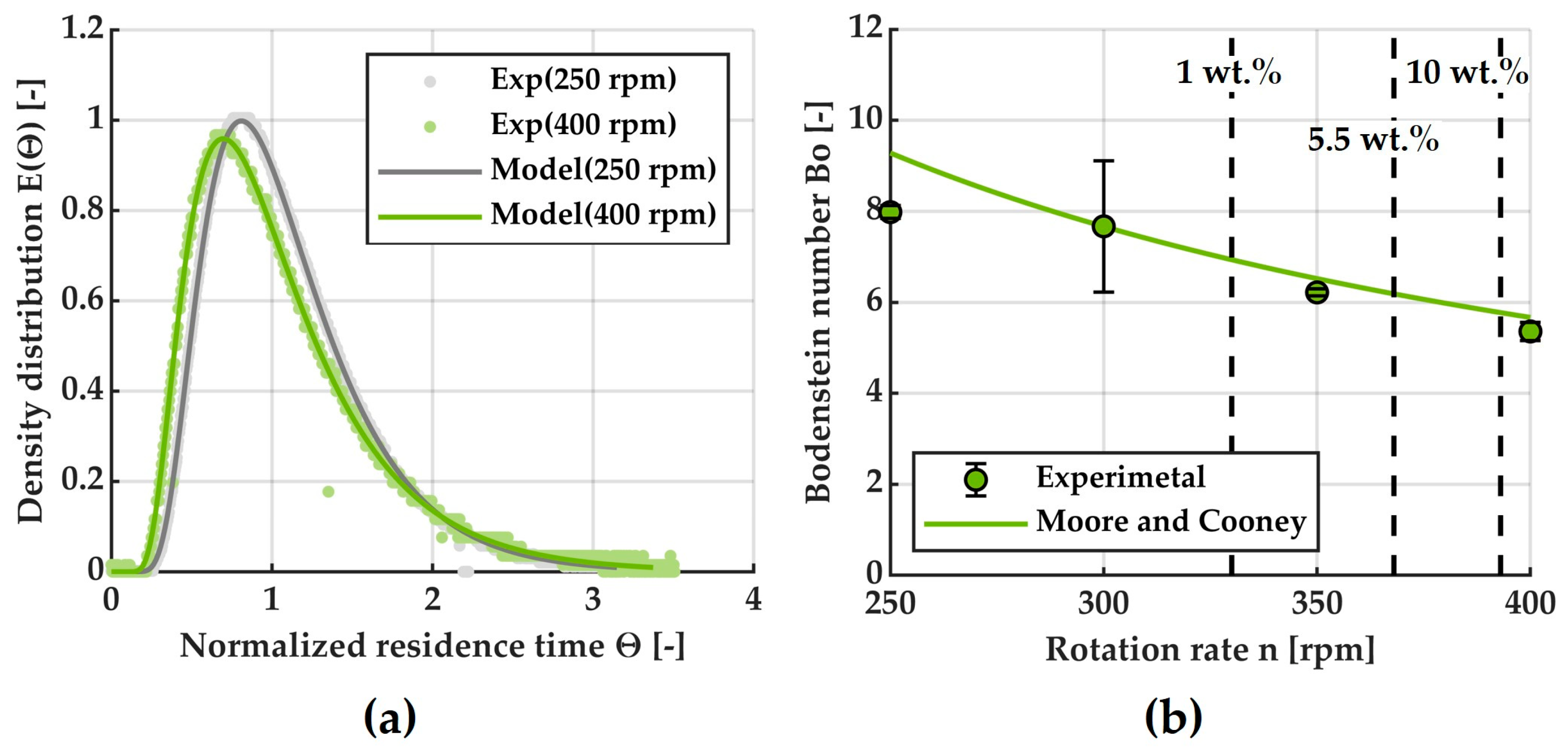
The suitability of the one-zone cell model (cf. Section 2.3.2) to reproduce the measured RTD_Ls is exemplarily depicted for the radius ratio $\eta$ = 0.7 and particle-free solution in Figure 8a. It shows the impulse responses for two operating points that covered the just-suspended rotation rates in a broad range. As can be seen, the model reproduced the experimental data very well. Accordingly, the assumption of perfect mixing of the liquid phase inside the vortices was valid. Furthermore, the rotation rate increase showed a slight increase in the axial dispersion only. Figure 8b shows this effect in more detail on the basis of the Bodenstein numbers within this range of rotation rates. In addition, the results were compared with an empirical correlation for the Bodenstein number in the Taylor–Couette system of Moore and Cooney [11] described by Equation (19).

$$B{o}^{-1}=7.2\cdot {10}^{-3}{\left(\frac{d}{r_i}\right)}^{-0.28}\cdot \left(\frac{2d}{L}\right)\cdot R{e}_{ax}{}^{-0.83}\cdot R{e}_{\theta }^{1.05}$$

(19)

The correlation can describe the Bodenstein numbers with sufficient accuracy. The RTD_L is quite broad and far from plug flow conditions for these operating points. With the Bodenstein numbers achieved, the residence time behavior is comparable to an MSMPR cascade of two to four vessels, which matches the amount commonly employed in crystallization processes [4]. In this respect, the TCC is convincing because the particles are suspended more gently than with conventional stirrers [12], and only one apparatus is required. Accordingly, the effort required for operation is reduced, and the challenging transfer of the suspension from vessel to vessel is omitted [7].

Considering the just-suspended rotation rates for the different mass fractions (dashed lines in Figure 8b) confirmed the assumption that the RTD_L changes only slightly due to the change in the required rotation rate caused by the expected increase in the mass fraction in a crystallization process. Therefore, at a fixed radius ratio, it is possible to operate the apparatus “on the safe side” with respect to the suspension without significant broadening in the RTD_L.

3.4. Prediction of Liquid Phase Residence Time Distribution in a Just-Suspended State

The results so far show that the requirement of complete particle suspension decisively determines the achievable RTD_L in the TCC. Depending on the apparatus geometry, operation in TTVF or WTVF is required, characterized by high axial dispersion. For design purposes, it is, therefore, useful to be able to predict the attainable RTD_L in the just-suspended state. For this purpose, the calculation procedure depicted in Figure 9, which links the just-suspended correlation established in this study (Equation (18)) to the correlation of Moore and Cooney [11] (Equation (19)), is proposed.

The procedure is as follows: As a first step, the target variables resulting from the crystallization process, i.e., volume flow rate $\dot{V}$, mass fraction $w_{solid}$, and median particle size $x_{50,3}$, are defined as inputs. Depending on the material system and its crystallization kinetics, the residence time $\tau$, necessary to achieve the defined particle properties, can be estimated. In combination with the volume flow rate, the required volume of the TCC is then calculable. The degrees of freedom that can be varied for this purpose are, e.g., the apparatus’s length $L$ and the radius ratio $\eta$ as inputs—making the radii of stator and rotor dependent variables. With this, the just-suspended rotational Reynolds number $R{e}_{\theta ,js}$ and, eventually, the Bodenstein number $Bo$ can be calculated. Then, as the final step, it is to be decided whether the TCC is a proper choice regarding its RTD_L. to achieve the targeted PSD. For this, the effect of $Bo$ on the PSD has to be quantified in another study.

To verify this method, we applied it in a slightly modified way along the apparatus at hand in this study. The available parameter space was limited by the constant apparatus length so that the residence time was not fixed. The particle size and mass fraction were set constant to $x_{50,3}$ = 348.82 µm ($Ar$ = 80.75) and $w_{solid,ala}$ = 5.5 wt.%, respectively. This seemed to be reasonable since the influences on $R{e}_{\theta ,js}$ were minor. The radius ratio was varied in the range $\eta$ = 0.5–0.84 by changing the rotor radius while keeping the stator radius set constant at $r_o$ = 26.8 mm. The volume flow rates were calculated from the two axial Reynolds numbers $R{e}_{ax}$ = 3.92 and $R{e}_{ax}$ = 15.67. The results of the prediction are shown in Figure 10. The experiments with the radius ratios and rotation rates listed in

Table 4. Radius ratios, rotation rates, and respective rotational Reynolds numbers for validating the prediction of the Bodenstein number in the just-suspended state. The particle size fraction 200–315 µm was used at a mass fraction of $w$ = 5.5 wt.%.

Radius Ratio η (-)	Rotation Rate $\mathit{n}$ (rpm)	Rotational Reynolds Number $\mathit{R}{\mathit{e}}_{\mathsf{\theta }}$ (-)	Volume Flow Rate $\dot{\mathit{V}}$ ($\mathit{R}{\mathit{e}}_{\mathit{a}\mathit{x}}$ = 3.92/15.67) (mL·min−1)
0.5	600	8256	-/82
0.7	400	4610	23/92
0.84	250	1854	25/99.5

were used for validation.

As expected, the Bodenstein number in the just-suspended state increased for increasing radius ratios since, as described in the previous section, the rotational Reynolds number decreased, displayed by the additional x-axis on top. While at a radius ratio of $\eta$ = 0.5, the residence time behavior of a continuous stirred tank was almost achieved, the backmixing could be significantly reduced when $\eta$ was increased.

Furthermore, the RTD_L also became narrower by increasing the volume flow $\dot{V}$ or the axial Reynolds number $R{e}_{ax}$ since the convective mass transport increased significantly more than the dispersive component, which was already evident from the model of Moore and Cooney [11]. However, it must be taken into account that the increase in the axial Reynolds number also reduced the residence time $\tau$; in the case of quadrupling of $R{e}_{ax}$ investigated here, $\tau$ was reduced to a quarter. To meet this challenge, the crystallizer length and the radii of both the rotor and stator could be increased while maintaining a high radius ratio.

Comparing the prediction with the experimental data showed that both correlations used for this purpose had sufficient accuracy and described the system well. Therefore, the simplification of using the solution viscosity rather than the apparent suspension viscosity in the calculations seemed to be valid from a viewpoint of design optimization.

At the radius ratios $\eta$ = 0.5 and 0.7, no effect of the particles on the RTD_L was discernible. This can be explained by the fact that the vortex boundaries were already locally strongly disrupted by the turbulence in the TTVF present here, which agrees with the results of Resende et al. [25]. However, the significant difference between the Bodenstein numbers for the radius ratio $\eta$ = 0.84 is remarkable, showing an increase in axial dispersion due to the presence of particles. The WTVF regime was present at this operating point, and the vortex boundaries allowed significantly less mass transport between two adjacent vortices. In this condition, particles that do not follow the streamlines and break the vortex boundaries can consequently increase the intervortex mass transfer [20].

In an actual continuous crystallization, an axial gradient will occur in the particle mass fraction and size. This might reduce the broadening of the RTD_L by the particles since smaller particles can follow the streamlines better and the vortex breakthrough would be less pronounced [20]. Interestingly, for $\eta$ = 0.84, the experimentally determined Bodenstein number for the particle-free flow significantly exceeded the predicted value, while $Bo$ of the particle-laden flow agreed with the prediction. Giordano et al. [18] reported similar results. They concluded that for decreasing turbulence outside the TTVF, the bypass flow increasingly affects the RTD_L since the intensity of local mixing decreases. Thereby, the bypass current depends on the drift velocity ratio (see Section 2.3.2), which can show significant differences between different Taylor–Couette apparatuses [12,19]. Therefore, it is possible that in the experiments of Moore and Cooney [11], a more intense bypass current increased dispersion compared to the data presented here. However, since the drift velocity ratio was not part of these two studies, this hypothesis cannot be verified.

4. Conclusions and Outlook

In this study, we investigated the relationship between particle suspension and achievable liquid phase residence time distribution (RTD_L) in a Taylor–Couette crystallizer (TCC). The system was characterized by flexibility in terms of local and global mixing, which were, however, coupled for a given geometry. An improvement of the local mixing or the suspension by the rotational Reynolds number is always accompanied by a broadening of the RTD_L. Accordingly, the effects on the just-suspended rotational Reynolds number were determined as the lower limit of the operating window.

It was demonstrated that this Reynolds number was mainly influenced by the radius ratio between the rotor and stator and therewith design of the TCC. This resulted in just-suspended states achieved in the flow regimes of turbulent Taylor vortex flow up to wavy Taylor vortex flow. With this, it was shown that a TCC for cooling crystallization allowed a flexible application. Depending on the geometry selected, the axial dispersion is adjustable from almost complete back-mixing to a narrow RTD_L by adjusting the process parameter rotation rate and volume flow rate. Furthermore, it was demonstrated that the achievable RTD_L in the just-suspended state in terms of the Bodenstein number was predictable. For this, a correlation for the just-suspended rotational Reynolds number was established and connected with another correlation for the Bodenstein number already known from the literature. A calculation sequence was then proposed for a design optimization towards a maximized Bodenstein number in a just-suspended state.

In future work, the applicability to a different material system should be determined. Therefore, the effect of the substance-specific parameter viscosity and density difference between solution and particles, postulated in the correlation by the Archimedes number, should be validated. Furthermore, a correction factor could be integrated for varying particle shapes, whereby it can be expected that with increasing deviation from spherical shape, the degree of suspension will be enhanced [40].

The solid phase residence time distribution should be investigated since it describes the variability in the growth times of the crystals. In addition, a cooling concept has to be developed that takes into account the variability of the RTD_L, allowing an optimal setting of the supersaturation for the cooling crystallization. With the help of this knowledge, the influencing variables for crystallization can then be precisely adjusted.

The study presented here demonstrated that a TCC shows potential for use in cooling crystallization. While the achievable RTD_L cannot match the plug flow conditions of other crystallizers, the TCC stands out for its combination of intense and uniform suspension and adjustable RTD_L.

References

1. Cote, A.; Erdemir, D.; Girard, K.P.; Green, D.A.; Lovette, M.A.; Sirota, E.; Nere, N.K. Perspectives on the Current State, Challenges, and Opportunities in Pharmaceutical Crystallization Process Development. Cryst. Growth Des. 2020, 20, 7568–7581. [Google Scholar] [CrossRef]
2. Orehek, J.; Teslić, D.; Likozar, B. Continuous Crystallization Processes in Pharmaceutical Manufacturing: A Review. Org. Process Res. Dev. 2021, 25, 16–42. [Google Scholar] [CrossRef]
3. Kleinebudde, P.; Khinast, J.; Rantanen, J. Continuous Manufacturing of Pharmaceuticals; John Wiley & Sons Ltd.: Hoboken, NJ, USA, 2017; ISBN 1119001331. [Google Scholar]
4. Wood, B.; Girard, K.P.; Polster, C.S.; Croker, D.M. Progress to Date in the Design and Operation of Continuous Crystallization Processes for Pharmaceutical Applications. Org. Process Res. Dev. 2019, 23, 122–144. [Google Scholar] [CrossRef]
5. Acevedo, D.; Yang, X.; Liu, Y.C.; O’Connor, T.F.; Koswara, A.; Nagy, Z.K.; Madurawe, R.; Cruz, C.N. Encrustation in Continuous Pharmaceutical Crystallization Processes—A Review. Org. Process Res. Dev. 2019, 23, 1134–1142. [Google Scholar] [CrossRef]
6. Zhang, D.; Xu, S.; Du, S.; Wang, J.; Gong, J. Progress of Pharmaceutical Continuous Crystallization. Engineering 2017, 3, 354–364. [Google Scholar] [CrossRef]
7. Cui, Y.; O’Mahony, M.; Jaramillo, J.J.; Stelzer, T.; Myerson, A.S. Custom-Built Miniature Continuous Crystallization System with Pressure-Driven Suspension Transfer. Org. Process Res. Dev. 2016, 20, 1276–1282. [Google Scholar] [CrossRef]
8. Termühlen, M.; Etmanski, M.M.; Kryschewski, I.; Kufner, A.C.; Schembecker, G.; Wohlgemuth, K. Continuous slug flow crystallization: Impact of design and operating parameters on product quality. Chem. Eng. Res. Des. 2021, 170, 290–303. [Google Scholar] [CrossRef]
9. Ibáñez-González, M.J.; Cooney, C.L. Studies on protein adsorption in a vortex flow reactor. Process Biochem. 2007, 42, 1592–1601. [Google Scholar] [CrossRef]
10. Schrimpf, M.; Esteban, J.; Warmeling, H.; Färber, T.; Behr, A.; Vorholt, A.J. Taylor-Couette reactor: Principles, design, and applications. AIChE J. 2021, 67, e17228. [Google Scholar] [CrossRef]
11. Moore, C.M.V.; Cooney, C.L. Axial dispersion in Taylor-Couette flow. AIChE J. 1995, 41, 723–727. [Google Scholar] [CrossRef]
12. Giordano, R.C.; Giordano, R.L.C.; Prazeres, D.; Cooney, C. Analysis of a Taylor–Poiseuille vortex flow reactor—I: Flow patterns and mass transfer characteristics. Chem. Eng. Sci. 1998, 53, 3635–3652. [Google Scholar] [CrossRef]
13. Kacker, R.; Regensburg, S.I.; Kramer, H.J. Residence time distribution of dispersed liquid and solid phase in a continuous oscillatory flow baffled crystallizer. Chem. Eng. J. 2017, 317, 413–423. [Google Scholar] [CrossRef]
14. Lawton, S.; Steele, G.; Shering, P.; Zhao, L.; Laird, I.; Ni, X.-W. Continuous Crystallization of Pharmaceuticals Using a Continuous Oscillatory Baffled Crystallizer. Org. Process Res. Dev. 2009, 13, 1357–1363. [Google Scholar] [CrossRef]
15. Coles, D. Transition in circular Couette flow. J. Fluid Mech. 1965, 21, 385–425. [Google Scholar] [CrossRef] [Green Version]
16. Desmet, G.; Verelst, H.; Baron, G.V. Local and global dispersion effects in Couette-Taylor flow—I. Description and modeling of the dispersion effects. Chem. Eng. Sci. 1996, 51, 1287–1298. [Google Scholar] [CrossRef]
17. Nemri, M.; Cazin, S.; Charton, S.; Climent, E. Experimental investigation of mixing and axial dispersion in Taylor–Couette flow patterns. Exp. Fluids 2014, 55, 1769. [Google Scholar] [CrossRef] [Green Version]
18. Giordano, R.; Giordano, R.; Prazeres, D.; Cooney, C. Analysis of a Taylor–Poiseuille vortex flow reactor—II: Reactor modeling and performance assessment using glucose-fructose isomerization as test reaction. Chem. Eng. Sci. 2000, 55, 3611–3626. [Google Scholar] [CrossRef]
19. Wereley, S.T.; Lueptow, R.M. Velocity field for Taylor–Couette flow with an axial flow. Phys. Fluids 1999, 11, 3637–3649. [Google Scholar] [CrossRef] [Green Version]
20. Dherbécourt, D.; Charton, S.; Lamadie, F.; Cazin, S.; Climent, E. Experimental study of enhanced mixing induced by particles in Taylor–Couette flows. Chem. Eng. Res. Des. 2016, 108, 109–117. [Google Scholar] [CrossRef] [Green Version]
21. Richter, O.; Hoffmann, H.; Kraushaar-Czarnetzki, B. Effect of the rotor shape on the mixing characteristics of a continuous flow Taylor-vortex reactor. Chem. Eng. Sci. 2008, 63, 3504–3513. [Google Scholar] [CrossRef]
22. Syed, A.; Früh, W.-G. Modelling of mixing in a Taylor-Couette reactor with axial flow. J. Chem. Technol. Biotechnol. 2003, 78, 227–235. [Google Scholar] [CrossRef]
23. Ma, J.; Cooney, C.L. Application of vortex flow adsorption technology to intein-mediated recovery of recombinant human alpha1-antitrypsin. Biotechnol. Prog. 2004, 20, 269–276. [Google Scholar] [CrossRef] [PubMed]
24. Resende, M.M.; Tardioli, P.W.; Fernandez, V.M.; Ferreira, A.; Giordano, R.; Giordano, R.C. Distribution of suspended particles in a Taylor–Poiseuille vortex flow reactor. Chem. Eng. Sci. 2001, 56, 755–761. [Google Scholar] [CrossRef]
25. Resende, M.M.; Vieira, P.G.; Sousa, R., Jr.; Giordano, R.L.C.; Giordano, R.C. Estimation of mass transfer parameters in a Taylor-Couette-Poiseuille heterogeneous reactor. Braz. J. Chem. Eng. 2004, 21, 175–184. [Google Scholar] [CrossRef]
26. Ibáñez-González, M.J.; Mazzuca-Sobczuk, T.; Redondo-Miranda, R.M.; Molina-Grima, E.; Cooney, C.L. A novel vortex flow reactor for the purification of B-phycoerythrin from Porphyridium cruentum. Chem. Eng. Res. Des. 2016, 111, 24–33. [Google Scholar] [CrossRef]
27. Rida, Z.; Cazin, S.; Lamadie, F.; Dherbécourt, D.; Charton, S.; Climent, E. Experimental investigation of mixing efficiency in particle-laden Taylor–Couette flows. Exp. Fluids 2019, 60, 61. [Google Scholar] [CrossRef] [Green Version]
28. Wereley, S.T.; Lueptow, R.M. Inertial particle motion in a Taylor Couette rotating filter. Phys. Fluids 1999, 11, 325–333. [Google Scholar] [CrossRef]
29. Wohlgemuth, K.; Schembecker, G. Modeling induced nucleation processes during batch cooling crystallization: A sequential parameter determination procedure. Comput. Chem. Eng. 2013, 52, 216–229. [Google Scholar] [CrossRef]
30. Borrero-Echeverry, D.; Crowley, C.J.; Riddick, T.P. Rheoscopic fluids in a post-Kalliroscope world. Phys. Fluids 2018, 30, 87103. [Google Scholar] [CrossRef]
31. Lührmann, M.-C.; Termühlen, M.; Timmermann, J.; Schembecker, G.; Wohlgemuth, K. Induced nucleation by gassing and its monitoring for the design and operation of an MSMPR cascade. Chem. Eng. Sci. 2018, 192, 840–849. [Google Scholar] [CrossRef]
32. Hergeth, W.-D. On-Line Monitoring of Chemical Reactions. In Ullmann’s Encyclopedia of Industrial Chemistry; Wiley-VCH Verlag GmbH & Co., KGaA: Weinheim, Germany, 2000; ISBN 3527306730. [Google Scholar]
33. Ferreira, L.A.; Macedo, E.A.; Pinho, S.P. Solubility of amino acids and diglycine in aqueous–alkanol solutions. Chem. Eng. Sci. 2004, 59, 3117–3124. [Google Scholar] [CrossRef]
34. Deutsches Institut für Normung e.V. DIN 66165-1, Partikelgrößenanalyse—Siebanalyse—Teil 1: Grundlagen; Beuth Verlag GmbH: Berlin, Germany, 2022. [Google Scholar]
35. Heisel, S.; Kovačević, T.; Briesen, H.; Schembecker, G.; Wohlgemuth, K. Variable selection and training set design for particle classification using a linear and a non-linear classifier. Chem. Eng. Sci. 2017, 173, 131–144. [Google Scholar] [CrossRef]
36. Heisel, S.; Rolfes, M.; Wohlgemuth, K. Discrimination between Single Crystals and Agglomerates during the Crystallization Process. Chem. Eng. Technol. 2018, 41, 1218–1225. [Google Scholar] [CrossRef]
37. Zwietering, T. Suspending of solid particles in liquid by agitators. Chem. Eng. Sci. 1958, 8, 244–253. [Google Scholar] [CrossRef]
38. Backhaus, K.; Erichson, B.; Plinke, W.; Weiber, R. Multivariate Analysemethoden; Springer: Berlin/Heidelberg, Germany, 2016; ISBN 978-3-662-46075-7. [Google Scholar]
39. Ruzicka, M.C. On dimensionless numbers. Chem. Eng. Res. Des. 2008, 86, 835–868. [Google Scholar] [CrossRef]
40. Schubert, H. Handbuch der Mechanischen Verfahrenstechnik; John Wiley & Sons: Hoboken, NJ, USA, 2012; ISBN 3527305777. [Google Scholar]
41. Steenweg, C.; Seifert, A.I.; Schembecker, G.; Wohlgemuth, K. Characterization of a Modular Continuous Vacuum Screw Filter for Small-Scale Solid–Liquid Separation of Suspensions. Org. Process Res. Dev. 2021, 25, 926–940. [Google Scholar] [CrossRef]
42. Baerns, M.; Behr, A.; Brehm, A.; Gmehling, J.; Hinrichsen, K.-O.; Hofmann, H.; Palkovits, R.; Onken, U.; Renken, A. Technische Chemie; Zweite, Erweiterte Auflage; Wiley-VCH: Weinheim, Germany, 2013; ISBN 3527330720. [Google Scholar]
43. Kraume, M. Transportvorgänge in der Verfahrenstechnik; Springer: Berlin/Heidelberg, Germany, 2012; ISBN 978-3-642-25148-1. [Google Scholar]
44. Esser, A.; Grossmann, S. Analytic expression for Taylor–Couette stability boundary. Phys. Fluids 1996, 8, 1814–1819. [Google Scholar] [CrossRef] [Green Version]
45. Nemri, M.; Charton, S.; Climent, E. Mixing and axial dispersion in Taylor–Couette flows: The effect of the flow regime. Chem. Eng. Sci. 2016, 139, 109–124. [Google Scholar] [CrossRef] [Green Version]
46. DiPrima, R.C.; Eagles, P.M.; Ng, B.S. The effect of radius ratio on the stability of Couette flow and Taylor vortex flow. Phys. Fluids 1984, 27, 2403. [Google Scholar] [CrossRef]
47. Nemri, M.; Climent, E.; Charton, S.; Lanoë, J.-Y.; Ode, D. Experimental and numerical investigation on mixing and axial dispersion in Taylor–Couette flow patterns. Chem. Eng. Res. Des. 2013, 91, 2346–2354. [Google Scholar] [CrossRef]
48. Lueptow, R.M.; Docter, A.; Min, K. Stability of axial flow in an annulus with a rotating inner cylinder. Phys. Fluids A Fluid. Dyn. 1992, 4, 2446–2455. [Google Scholar] [CrossRef] [Green Version]
49. Wereley, S.T.; Akonur, A.; Lueptow, R.M. Particle–fluid velocities and fouling in rotating filtration of a suspension. J. Membr. Sci. 2002, 209, 469–484. [Google Scholar] [CrossRef]
50. Sobolík, V.; Jirout, T.; Havlica, J.; Kristiawan, M. Wall Shear Rates in Taylor Vortex Flow. JAFM 2011, 4, 25–31. [Google Scholar] [CrossRef]
51. Ostilla-Mónico, R.; van der Poel, E.P.; Verzicco, R.; Grossmann, S.; Lohse, D. Boundary layer dynamics at the transition between the classical and the ultimate regime of Taylor-Couette flow. Phys. Fluids 2014, 26, 15114. [Google Scholar] [CrossRef]
52. Liepe, F. Stoffvereinigen in fluiden Phasen—Ausrüstungen und ihre Berechnung. In Verfahrenstechnische Berechnungsmethoden, 1st ed.; Weiß, S., Ed.; VCH Verl.-Ges: Weinheim, Germany, 1988; ISBN 3527262059. [Google Scholar]
Figure 1. Exemplary cumulative PSDs of the employed l-alanine particle fractions after wet sieving.
Crystals 12 01845 g001
Figure 2. Illustration of the employed set-up. (a) Schematic depiction. Current measurement probes were integrated at positions 1 and 2 to measure the RTDL. A three-way valve behind the TCC’s outlet could be used to convey either a circuit back into the feed vessel or a waste container. Operating and design parameters are shown in blue and orange, respectively. (b) Photograph of the TCC. The end plates were held in place by four steel rods. The motor was fixated on one end plate and connected to the rotor by a spring clutch.
Crystals 12 01845 g002
Figure 3. Photographs of the flow visualization experiments for w s o l i d , M i c a = 0.05 wt.%, η = 0.7, V ˙ = 92 mL∙min−1 and R e a x = 15.67. (a) Adjustment of the flow regime after a change in rotation rate from n = 25 rpm to n = 80 rpm. Existing wavy vortices retained their pattern and were displaced by newly forming turbulent wavy vortices. (b) Observed flow regimes; LCF is not shown. The corresponding videos are supplied in the Supplementary Materials as (a) S1 and (b) S2–S4.
Crystals 12 01845 g003
Figure 4. Rotational Reynolds numbers of the flow regime transitions for the different geometries. The axial Reynolds number was set constant at R e a x = 15.67, resulting in the volume flow rates V ˙ = 99.5, 92, and 82 mL∙min−1 for the ratios η = 0.84, 0.7, and 0.5, respectively.
Crystals 12 01845 g004
Figure 5. Photographs taken from below the apparatus showing different suspension states for the geometry η = 0.7, sieve fraction 315–400 µm, and solid content w s o l i d , a l a = 5.5 wt.%: (a) sediment formation between vortex pairs at n = 275 rpm, (b) complete suspension at n = 400 rpm. Moreover, for complete suspension, a settling area between the vortex pairs existed, where particles moved along the stator but remained for less than a second. The related videos are supplied in the Supplementary Materials as (a) Video S5 and (b) Video S6.
Crystals 12 01845 g005
Figure 6. Parity plot displaying the goodness of fit of the regression of the just-suspended rotational Reynolds number. The error bars indicate the 95% confidence intervals of the regressed data.
Crystals 12 01845 g006
Figure 7. Just-suspended rotational Reynolds numbers for different radius ratios, particle sizes, and mass fractions. The different colors depict the different mass fractions, while the symbols differentiate between the particle sizes. The dotted lines represent the predictions of R e ^ θ , j s (Equation (18)) for the smallest (small dots), medium (big dots), and largest (small dots) investigated particle sizes and mass fractions. The axial Reynolds number was set constant to R e a x = 15.67.
Crystals 12 01845 g007
Figure 8. Liquid phase residence time distributions for the radius ratio η = 0.7 and axial Reynolds number R e a x = 15.67 equaling a volume flow rate of V ˙ = 92 mL∙min−1 and hydrodynamic residence time of τ = 7.45 min. (a) Density distributions depicting the one-zone cell model fit of the experimental data. (b) Bodenstein numbers as a function of rotation rate. The error bars represent the standard deviation of two experiments. The solid curve results from the empirical correlation from Moore and Cooney [11]. The dashed lines display the just-suspended rotation rates for x 50 , 3 = 348.82 ± 5.50 µm and different particle mass fractions.
Crystals 12 01845 g008
Figure 9. Calculation procedure for optimizing the TCC’s design parameters regarding the achievable Bodenstein number B o in a just-suspended state. The input parameter volume flow rate V ˙ , particle mass fraction w s o l i d , and median particle size x 50 , 3 were predefined by the crystallization process. By varying the design parameter length L and radius ratio η , B o can be maximized. To decide whether the achievable Bo is sufficient to achieve the required PSD, the effect of B o on the PSD needs to be investigated in another study.
Crystals 12 01845 g009
Figure 10. The Bodenstein number B o of the liquid phase as a function of the radius ratio η for the two axial Reynolds numbers R e a x (distinguishable by color) for particle-free solution flow as well as for suspension flow ( x 50 , 3 = 348.82 µm; w s o l i d , a l a = 5.5 wt.%). The solid lines display the prediction calculated according to the procedure described in Figure 9.
Crystals 12 01845 g010