Prediction of Lattice Volumes of Crystal Samples by Computer Image Recognition on the X-ray Diffraction Patterns

Abstract

Computer image recognition (CIR) on the diffraction patterns of X-ray single crystal diffractometer was used to assist the analysis of the unit cell parameters in terms of lattice volume. This method can improve the prediction accuracy of unit cell parameters in the pre-experiment step since erroneous prediction by the software may occur for 5% tested crystal samples, which may critically affect the complete crystal data quality and cause unnecessary testing time. In the imaging processing, the diffraction pattern images saved as .img format files were firstly batch transferred into .jpg format with high quality for further treatment. Specific features of the crystal diffraction points or zones in the images were extracted for the recognition processing by color mode. The Findcontour algorithm and the Canny algorithm based on Gaussian filtering were used for the diffraction peak points and area detection. The relationship between the distribution of crystal diffraction points (DCDP) and the lattice volumes based on reciprocal lattice theory was established for the users to judge the reasonable location range of the lattice volumes. A Density model was proposed to correlate the dependence of the DCDP and the experimental data. Special crystal samples were chosen to test the CIR performance, and its accuracy for the lattice volume prediction was evaluated. The CIR method can be used for the assistance in the analysis of the lattice volume location range and for crystal structure solving.

1. Introduction

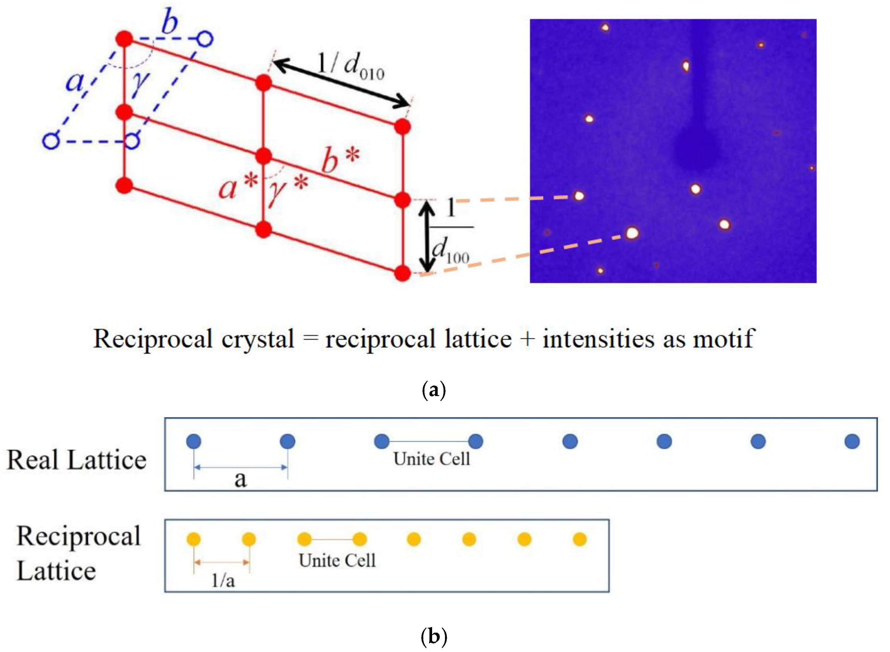
1.1. Reciprocal Lattice and Cell Parameters

Single crystal structures are key proofs for the characterization of crystalline materials. X-ray diffraction is widely used for analysis of crystal structures [1]. In order to easily understand the relationship between the diffraction information and the crystal structure by mathematic treatment, reciprocal lattice is introduced which is transferred from the real lattice by Fourier transformation. The X-ray diffraction pattern of a real lattice is illustrated by its reciprocal lattice for easily handling by mathematic tool, as shown in Figure 1. The product of the real lattice volume and the reciprocal lattice equals to 1 (V·V * = 1, V: real lattice, V = a × b × c ų; V *: reciprocal lattice, V * = a * × b * × c * ų). An experienced user can evaluate the location range of the real lattice volume from the diffraction pattern composed of many diffraction peaks by eyes. In this study, the computer image recognition (CIR) is employed to evaluate the real lattice volume base on the reciprocal theory of crystals.

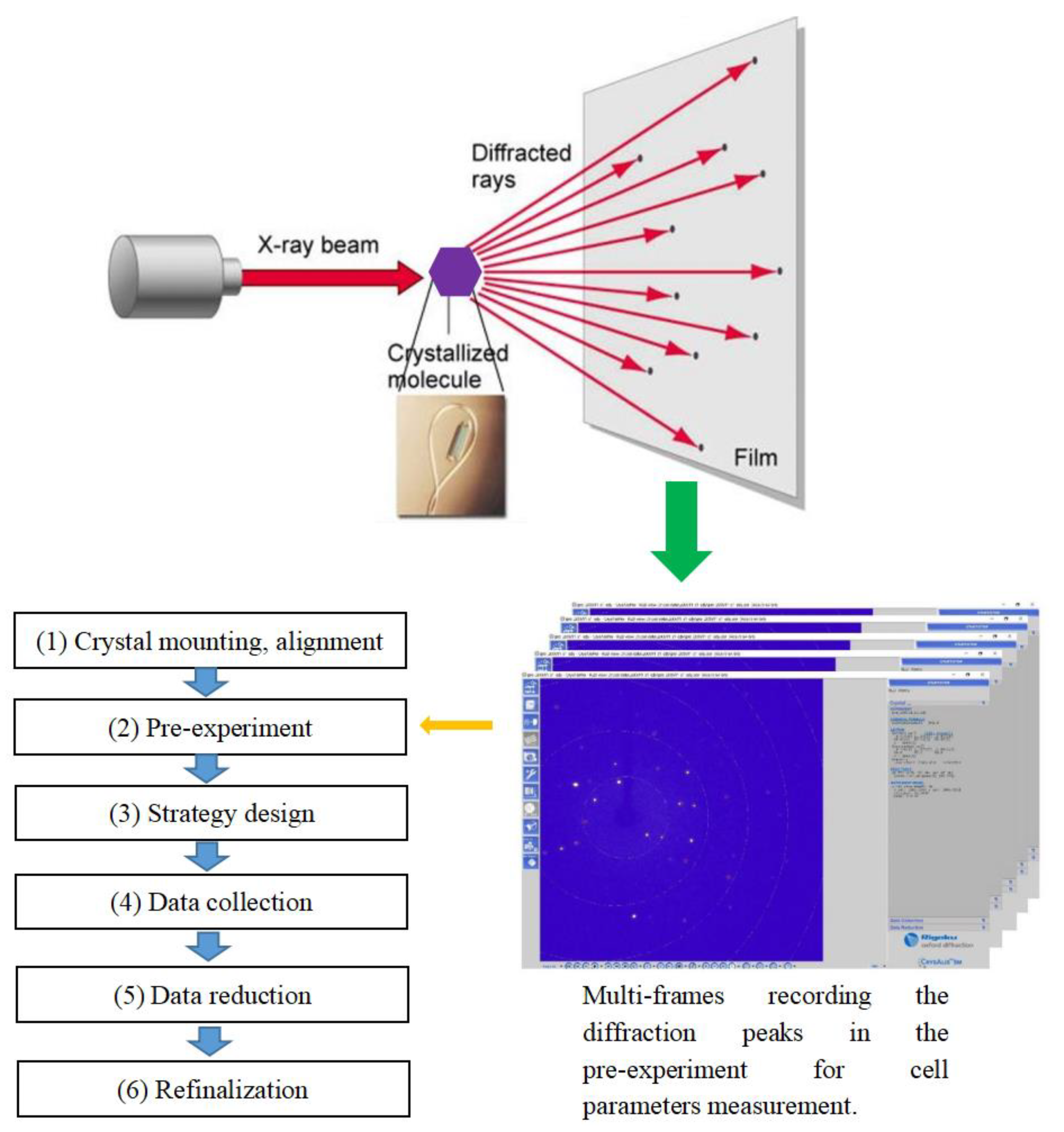
1.2. X-ray Diffraction

X-ray diffraction is a powerful tool to determine the crystalline structures of single crystal samples. The complete procedure of the crystalline data collection on the single crystal X-ray diffractometer (SCXRD) in our lab includes six sequential steps: (1) sample mounting, (2) pre-experiment, (3) strategy choice, (4) complete data collection, (5) data reduction, and (6) re-finalization. The data collected in the pre-experiment step play an important role to determine the consumed time and quality of the completely collected data, as shown in Figure 2. The pre-experiment window in the GUI provides direct feedback of the unit cell parameters, which normally costs 10 min of operation for each crystal sample. The collection strategy is based on the unit cell parameters and lattice asymmetry with a limited number of images recording diffraction peaks in the pre-experiment stage. The pre-experiment window provides direct feedback of the unit cell, intensity statistics, and the set-up for the automatic data collection as reference. However, the software sometimes gives incorrect unit cell parameters if the crystal sample has a low quality, or large lattice volume, or a twin lattice, which will mislead the users to choose an uncorrected strategy to collect the complete data costing much more unnecessary time. In this case, we cannot solve the correct crystalline structures, or will obtain data with incomplete degree in the (4) step (Figure 2). This SCXRD works with a four-circle sample holder, which named as θ, χ, ω, φ circle, respectively. On the diffraction image, each diffraction peak has a unique [θ, χ, ω, φ] value to identify its position in the reciprocal space [2].

1.3. Computer Image Recognition on the Diffraction Pattern

The indexation of the diffraction pattern will be performed in the pre-experiment to calculate the cell parameters such as a, b, c, and V. Among them, the lattice volume V is suitable for predication by computer image recognition (CIR) method since it has close relationship with the dispersion of the diffraction pattern [3,4,5]. According to the empirical prediction of the users for thousands of crystal samples, the workstation program will output confused information even wrong unit cell parameters for about 5% crystal samples from the data. Especially for a low-quality crystal sample (or large-cell-volume, or twin sample), a default unit cell as the output may be incorrect. To address this problem, we propose the CIR method in order to assist the users for the judgement on the diffraction pattern, which can help increasing the prediction precision of the unit cell parameters [6]. It is known that the cell parameters, especially the cell volume, are in close correlation to the distribution concentration of the diffraction pattern, which are shown as circle dots on the diffraction window in the program GUI (Figure 3). The diffraction pattern profile allows the user to establish a correlation between the distribution concentration (or density) and the unit cell volume. It can be seen that a smaller lattice volume has a widely scattered dispersion of the diffraction peaks (Figure 3a), while a larger lattice volume has a dense pattern of the centralized diffraction peaks (Figure 3b). This difference of the diffraction peak dispersion can be used as the predication experience of the CIR method. If the samples to be measured are of low quality, the software may give varieties of lattice volume values (Figure 3c) that mislead the users to choose correct strategies for the further data collection. Under this circumstance, CIR may play as an important tool for the users to locate the right range of the lattice volume (Insert table of Figure 3c).

2. Materials and Methods

2.1. Diffraction Data Collection

Single crystals of 30 samples were selected and detected on the X-ray diffractometer (Excalibur EOS, Rigaku). These samples, including organic molecules and metal-organic frameworks, had a mean index rate of 95% and about 330 diffraction images for each. The crystals were kept at 293.15 K during the data collection by the workstation program.

The program GUI is comprised of a few different areas, which include the tool area, diffraction/image display window, and button area, as shown in Figure 2. As soon as the one frame has been collected the automatic software will attempt to find the unit cell. Once a unit cell has been successfully found it will be displayed in the pre-experiment window, along with the information relating to the quality of the cell that shown in a percentage of the indexed reflections. As additional frames are recorded, the unit cell is re-determined and the pre-experiment is updated with the new (or improved) unit cell. The proposed data collection strategy is also displayed on the right section. Meanwhile, intensity statistics and a proposed exposure time for the data collection, which are dependent on the initially specified resolution and I/sig values, will be provided for the users. These can be altered during the pre-experiment, thereby updating the proposed strategy. The pre-experiment itself can be re-opened at any time by locating it in the load experiment dialogue window or locating the pre-experiment name.par file in the experiment folder.

The image list allows the users to open and save diffraction images. Ideal diffraction peaks should have a narrow sharp profile with no obvious humps on the side. In order to obtain the relationship between the crystal diffraction density and its volume, the crystal diffraction image for computer recognition must be batch obtained. The raw crystal diffraction data obtained from the diffractometer are in IMG format, and we cannot batch handle and obtain the data in this format. Therefore, we firstly converted them into a computer-recognizable JPG format implemented through python code. Next, we performed a series of image preprocessing, including grayscale conversion, filtering, edge processing, and dilation processing. Following this, a region of interest (ROI) is extracted, and the image of the region is segmented to extract the contour of the diffraction spot, and the area of each diffraction spot is calculated; finally, the diffraction density is calculated according to a certain algorithm. The image processing algorithm is based on OpenCV software [7].

2.2. The Distribution of Diffraction Points in Different Mode

CIR is a powerful tool to process and analyze images. In this work, traditional CIR technology was proposed to study the relationship between the distribution of crystal diffraction points (DCDP) and their lattice volumes. It should be noted that, since each crystal sample has different diffraction ability, the intensity of the diffraction peaks of one sample may be greatly different from other ones. Hence, we cannot treat all the samples’ patterns by one standard. In this processing, we used the ratio of the peak contribution in lightness and area at different zones in each diffraction image, which reflected the Density (relative DCDP ratio) of each sample. Typical diffraction images of a crystal sample are shown in Figure 4. The white circles in each image represent the 2θ contour lines, which are regarded as the indication of the diffraction resolution in the experiment. In the software different displaying mode with 3, 5, 7 concentric circles, respectively, can be selected to indicate the 2θ contour lines (Figure 4a–c). The CIR processing will be performed on different zones such as these concentric circles since they clearly mark the diffraction resolution as a fixed calibration. In fact, in the CIR processing the contour-line-like circles were used as the boundary lines to divide the diffraction zones of the DCDP for comparison. The diffraction peaks are illustrated as the bright spots on the blue background, and the DCDP circled in the ring area is different from the circle center, which is in accordance with the principle of diffraction spots distributed in the reciprocal space. The higher the diffraction intensity, the brighter the diffraction spots. In this paper, the term ‘Density’ is used herein to refer to the ratio of the total sum of the areas of the diffraction points in the ring to the total area of the diffraction spots of the whole image, which is equivalent to the ratio of the sum of the respective pixel points of these two parts in the CIR processing.

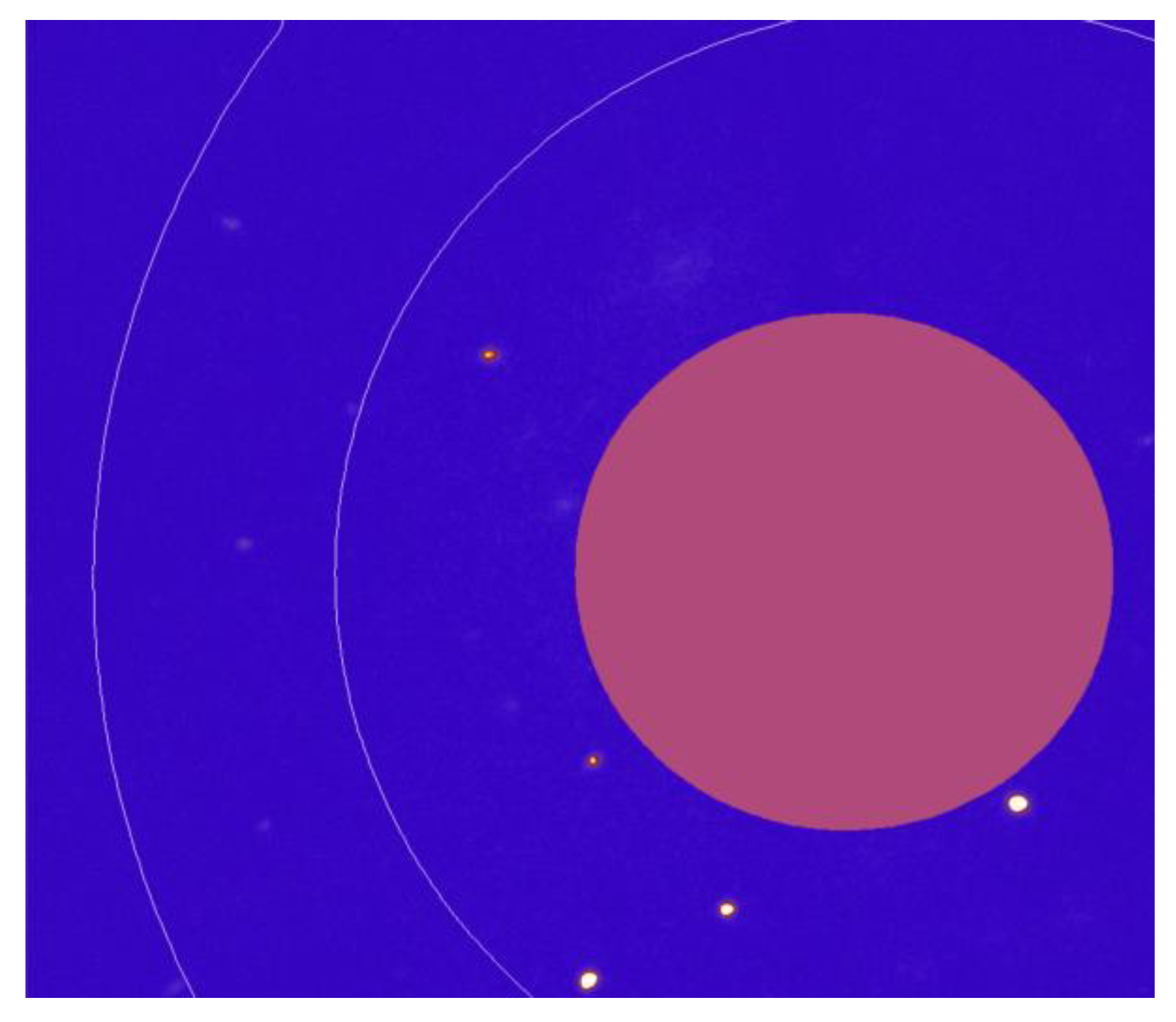
2.3. Image Preprocessing

The crystal diffraction image collected in this work is a colorful image in blue and white [8]. In the image, each pixel is composed of three basic components, namely R, G, and B, respectively. They are the three primary color components at the gray level, and each primary color component has 255 gray values forming the color combination. A grayscale image has the same gray values of the three primary color components. All the key information of a diffraction image can be expressed based on the color mode in gray values for the data extraction.

Based on this, we converted the colored images into grayscale image for the recognition processing. A typical colorful diffraction image converted to a grayscale image is shown in Figure 5a. Filtering processing is necessary to remove the noise from the background and to smooth the image. The simple average denoising principle is simple, but easy to fuzzy border after the noise reduction, and so it cannot be widely applied in image pre-processing [9]. In this work, Gaussian filtering was used for image pre-processing. The value of each pixel in the image was obtained by comparison between their weighted averaging value and the neighborhood pixel values. After the Gaussian filtering, the diffraction area was successfully extracted from the background, as shown in Figure 5b. The Canny algorithm is one of the most commonly-used methods for edge detection based on Gaussian filtering [10]. The Canny algorithm traverses the pixel points in the image, removes all non-edge points according to the gradient, and applies double thresholds to determine the edge points [11]. Canny algorithm was employed for the diffraction area edge detection, and the result is shown in Figure 5c. Next, the edge features of the pixels were dilated to highlight them for the subsequent extraction of diffraction area profiles [12]. The convolution kernel used in the dilation processing was based on a 3 × 3 matrix with the iteration number of 1. The diffraction image after the edge dilated treatment is shown in Figure 5d.

2.4. ROI of Image

After the preprocessing step, the annular region in the figure, namely the ROI [13], is identified by detecting the contour, as shown in Figure 6. The coordinate of the circle center was calculated and recorded as (X₀, Y₀). The detection method is to only detect the outer contour, which can exclude the contour detection of the diffraction area in the ring, and set the contour area threshold at the same time, which can exclude the interference of other contours. In this case, the detection rate is greatly improved.

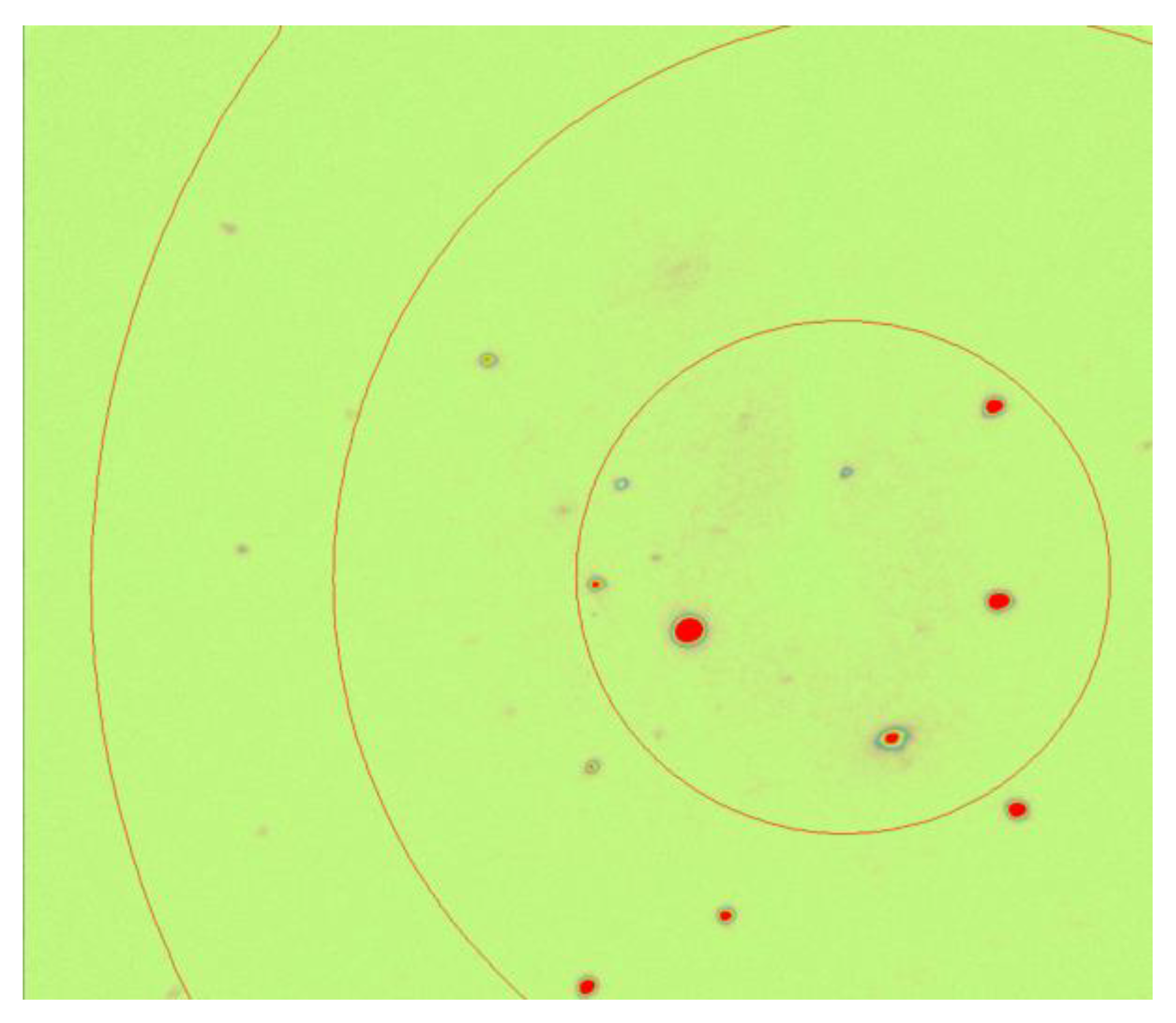
2.5. Image Segmentation

Currently, various methods are used for image segmentation, such as threshold segmentation, region segmentation, and color segmentation. In this work, color segmentation was used for the image process in [14]. An advantage of this method is that the parameters can be adjusted in real-time to find the optimal parameter values. In order to achieve this effect, the images are required to be converted from RGB space to HSV space in color mode [15]. The effect of the proposed color space is mainly to increase difference among the three tunnels; thus, the color information of images can be fully used [16]. Compared with RGB space, HSV space has saturated hue with independent values, which can accurately express the brightness, saturation, and chroma of pixels. The image in HSV space is shown in Figure 7.

Color segmentation decomposes an image according to the three parameters of hue, saturation, and lightness. Different segmentation effects can be achieved by setting the maximum and minimum thresholds by adjusting the three parameters [17]. In the GUI panel, six parameters to regulate the hue, saturation and lightness (each with min and max options) can be adjusted to display the segmentation effects. After comparison, the optimal thresholds of these parameters were found; thus, providing the best segmentation. A typical color segmentation image to prominently indicate the diffraction area is shown in Figure 8.

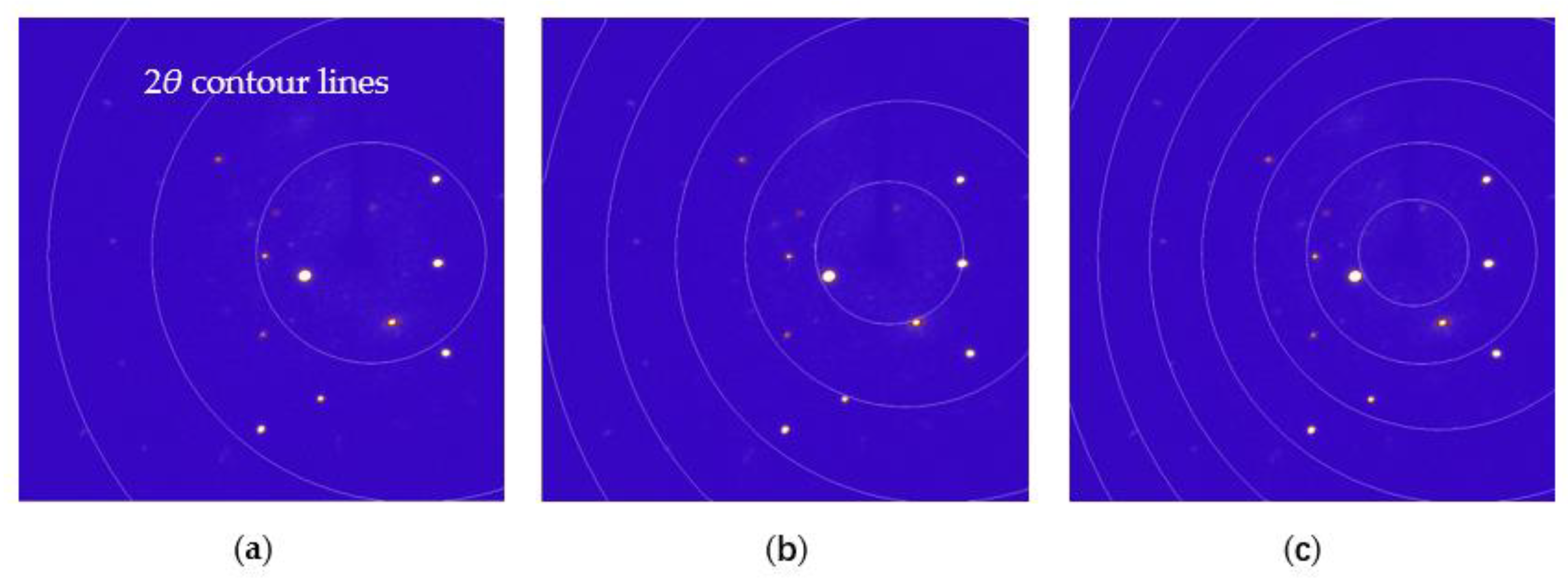
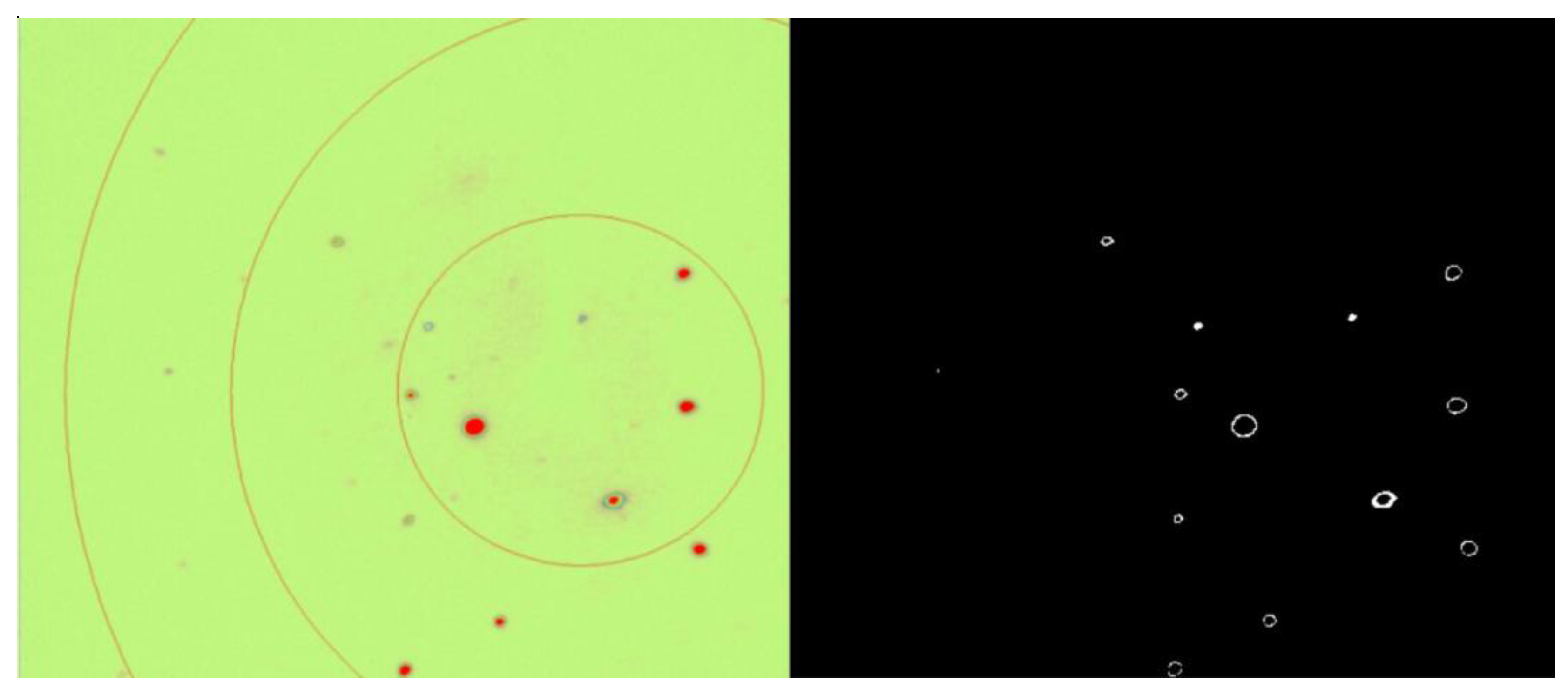
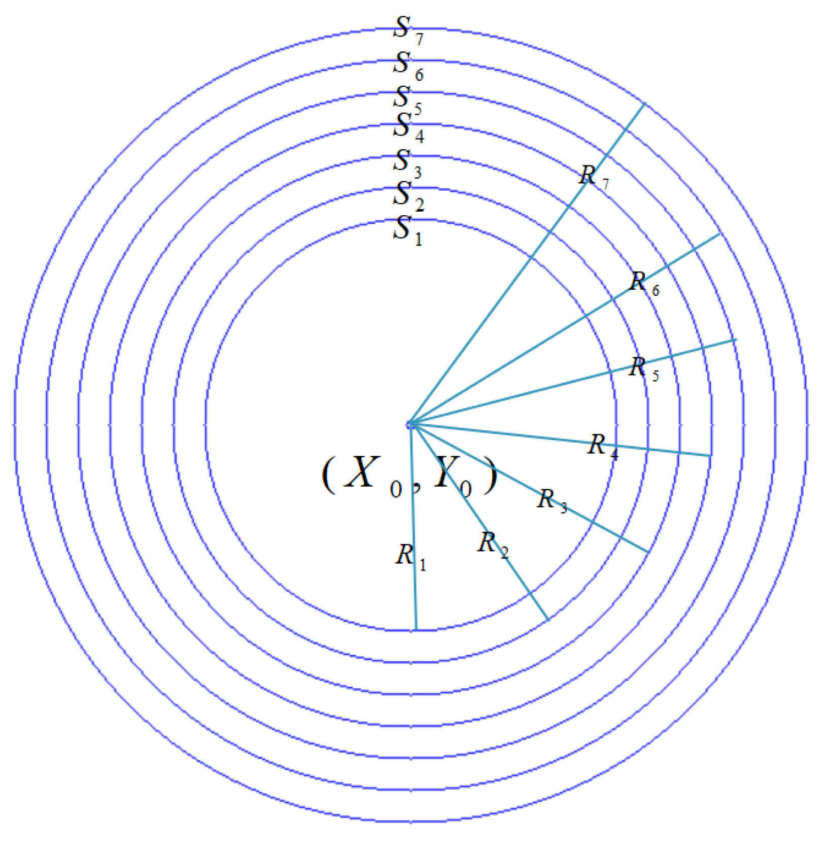
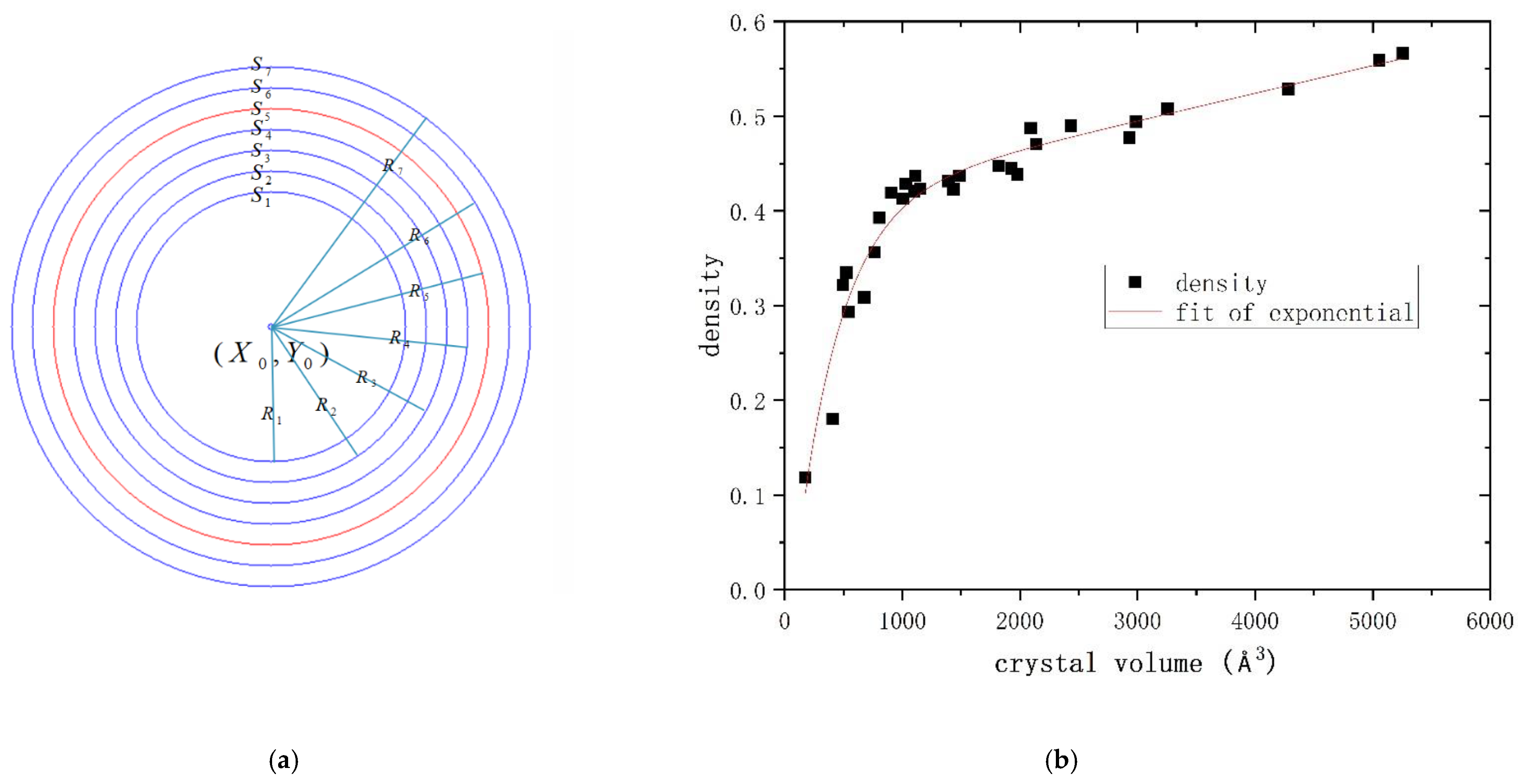
2.6. Contours Segmentation

After the image was segmented by the color segmentation method, only the information of the diffraction points was left in the image, as shown in Figure 8. In addition, the image preprocessing operations such as filtering, edge processing, and expansion processing were performed on the image. After that, the diffraction part of the image was extracted by the Findcontours function. After the contour was found, the Drawcontours function was used to draw the contour and to fill the interior. The green color was selected to be drawn and displayed in the source image. All the image processing related functions are referred to the OpenCV library (https://opencv.org/) (accessed on 1 January 2022). The contoured result of a diffraction image is shown in Figure 9. In the Findcontours method, the input image is usually a binary image processed by an edge detection algorithm, and the detected contour is represented as a point vector [18]. A contour is composed of a set of continuous point vectors. There are four retrieval modes to find the contours. The mode adopted in this work was to detect only the outermost contours, ignoring the inner contours contained in the outer contours. Based on this vision effect, the center coordinates of each diffraction zone were calculated and recorded as (X_i, Y_i) (i = 1, 2, 3, …). Meanwhile, the area of each diffraction point was calculated, and the results were recorded as S_j (j = 1, 2, 3, …). After that, all the diffraction zones on the image were precisely located by coordination.

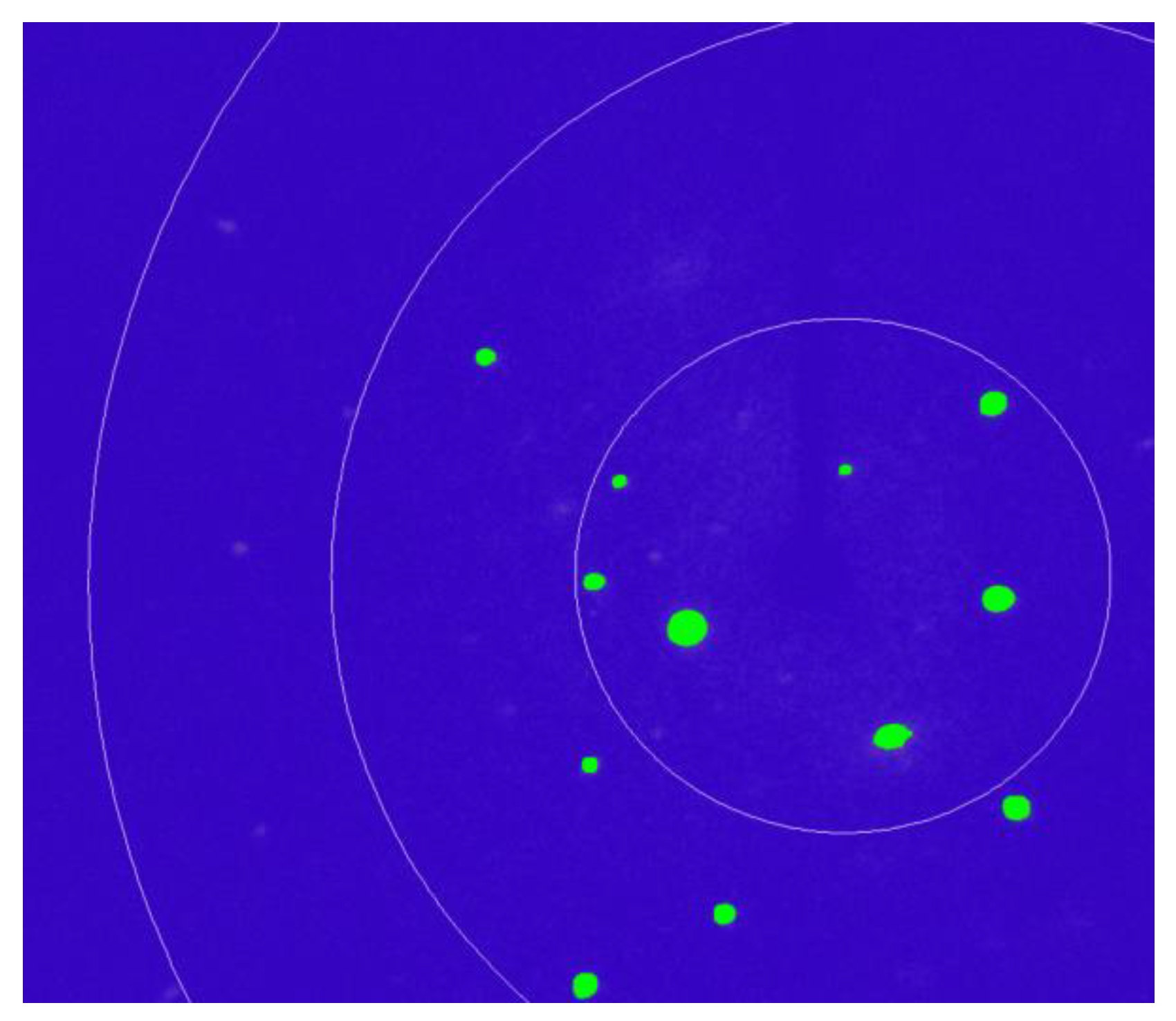
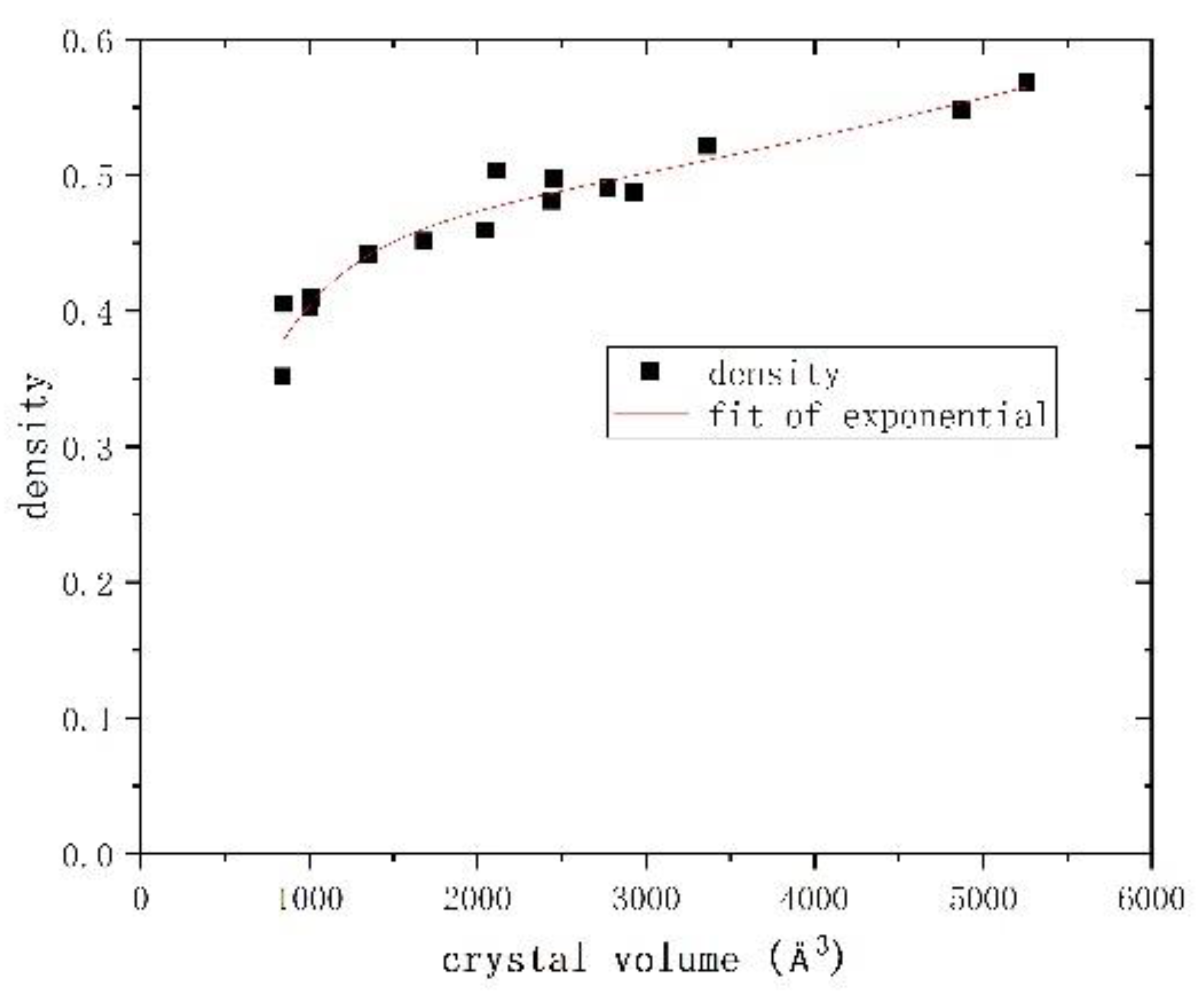
2.7. Density Calculation

In crystal diffraction experiments, hundreds of diffraction images are obtained for each crystal sample with different lattice volumes. The seven densities of these hundreds of diffraction images are averaged to obtain the seven final densities in this volume. In order to obtain the DCDP, the number of all pixels in the detected contour is calculated as the area of the contour.

Based on the series of ROI treatment, the Density model was required to divide the diffraction image into different circle zones to compare the Density difference and to calculate the DCDP. Firstly, the coordinate of the center of the ROI image was determined as the center of the model. Next, seven concentric circles with the center were drawn to find the best Density result, as shown in Figure 10. The size of the diffraction image selected in this work was fixed at 1024 pixels × 1024 pixels, which was desired to handle and was convenient to observe and store. Each circle line was tested to find the optional result for Density calculation, since the discrimination effect could not be well shown using the circled area if too large or too small. If the area of the ring is too small, the diffraction image of the crystal in some volumes will have no diffraction spots within the ring, while the area of the ring is too large, the ring will exceed the image range. After the many-time test, the smallest circle with 130 pixels in radius, while the largest circle with 250 pixels in radius was chosen with the ring spacing was 20 pixels because this was the best reasonable choice for the zone dividing. The distance between each diffraction point and the diffraction center was calculated by Equation (1):

$$d_i=\sqrt{{(x_i-x_0)}^2+{(y_i-y_0)}^2}$$

(1)

The difference of the DCDP in each circle (R_i) was compared by the relationship between R_i and d_i. On this basis, the total sum of the diffraction areas in the seven circles could be calculated. The total sum of all the diffraction areas in the diffraction image was represented by S, which were manually divided into concentric-circles such as the division effect in Figure 4c. Accordingly, the sum of the diffraction areas in the first ring in the Density model was S₁, the sum of the diffraction areas in the second ring is S₂, and so on S₃, S₄, S₅, S₆, S₇. Furthermore, the D_i value for the DCDP ratio by the seven intensities was introduced and given by Equation (2).

$$D_i=\frac{S_i}{S},i=1,2,3,\dots 7.$$

(2)

3. Results

In this work, CIR on about 10,000 diffraction images from 30 crystal samples was performed. Based on the CIR results, there is a functional correlation between the seven densities and the lattice volumes. The Origin software was used to perform the linear fitting on their relationships, and the R-squared was compared to judge the fitting effect. In the fitting results, D₅ had the best correlation for fitting the selected lattice volumes since its R-squared value is the closest to 1, and its Density model is shown in Figure 11a. In order to optimize the fitting effect, various function models in the Origin software were used to fit D₅, and the R-squared value were compared to evaluate the fitting effect. The results show that the R-squared value obtained by exponential fitting using the ExpDec2 function is the largest, which means the fitting effect is the best. Therefore, this function was selected as the final fitting function. The relationship between the lattice volume and the DCDP by D₅ correlation was drawn in Figure 11b. As can be seen, the experimental lattice data and the Density values for the crystal samples showed a nonlinear relationship from 174 to 5256 ų. After careful calculation and simulation, the relationship between the Density and lattice volume was established by exponential fitting treatment as follows:

$$D=-0.4969\times \exp (-\frac{V}{373.16})-6061.13\times \exp (-\frac{V}{2.07569E8})+6061.54$$

(3)

where D is the diffraction density of the crystal and V is the volume of the crystal. In the practical experiment, crystal samples are dominated with little lattice volumes (less than 5000 ų), hence there were plenty samples for CIR treatment in this lattice volume range.

This is because the D₅ value is corresponding to the 8.33° of the θ angle (2θ = 16.66°) as the resolution indicator line (also contour lines) on the diffraction pattern. Enough data could be collected below the θ angle at 10° on a Mo diffractometer for many kinds of crystal samples. When the θ angle is larger than 10°, the diffraction data play little roles to determine the data quality. The ROI result from the D₅ agreed well with the crystal diffraction mechanism.

4. Discussion

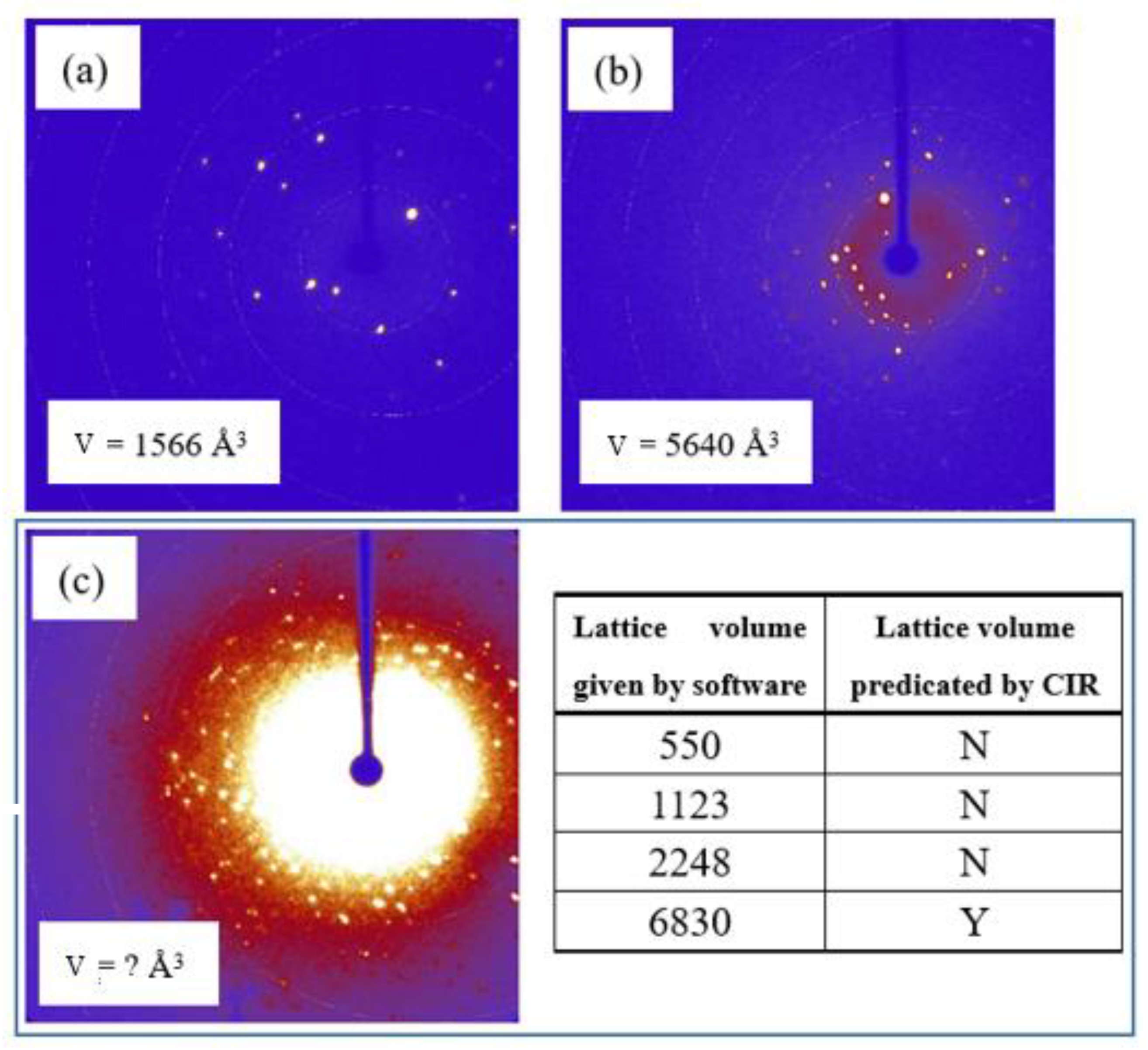
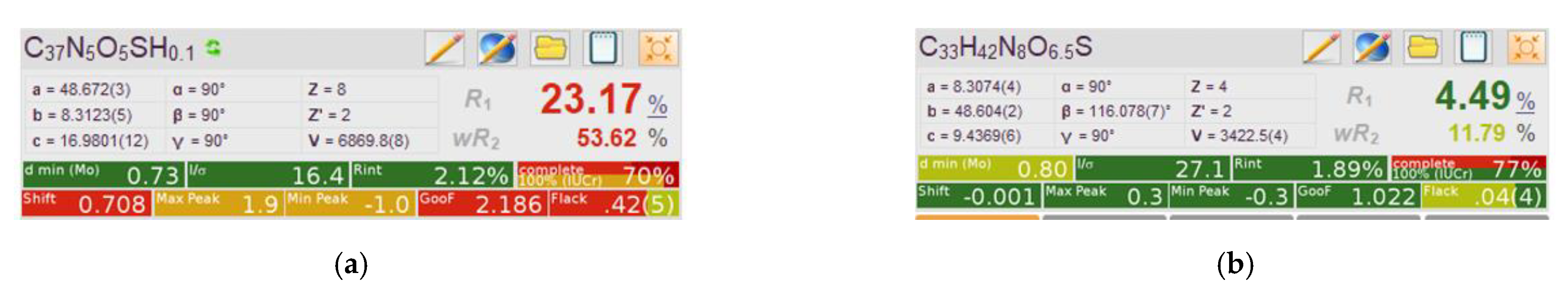
4.1. Assistance for Strategy Design in the Pre-Experiments

We took out 15 crystal samples with unknown volumes for evaluation the CIR performance. Their diffraction images were firstly transformed to obtain the DCDP ratio. Based on the exponential relationship between the lattice volume and the DCDP ratio, the unit cell volume value can be predicted in a reasonable range. The CIR predicted volumes for the 15 selected crystal samples were compared with the real cell parameters obtained by the data collection software and the result is listed in

Table 1. Selected crystal samples for CIR testing.

Sample Number	Density	Predicted Volume	Real Volume	Prediction Bias (%)
1	0.351564	699.35	842.48	16.9
2	0.405231	1022.88	852.38	20.0
3	0.402627	1000.75	1006.71	0.59
4	0.459351	1887.04	2047.8	7.85
5	0.441348	1482.47	1349.47	9.86
6	0.409692	1063.21	1013.7	4.88
7	0.503331	3287.41	2116.7	55.3
8	0.497459	3088.11	2450.6	26.0
9	0.487212	2743.76	2930.3	6.37
10	0.568281	5525.61	5259.1	5.07
11	0.481121	2542.93	2434.6	4.45
12	0.490568	2855.86	2772.7	2.99
13	0.521694	3914.21	3365.6	16.3
14	0.547753	4806.22	4872	1.35
15	0.451295	1687.65	1682.4	0.31

. The purpose of this paper is to predict reasonable lattice volumes of crystal samples through the CIR method, which provides a proper range of the lattice volumes in the pre-experiment step. This CIR assistance can effectively reduce the unnecessary experimental time in the data collection step for crystal samples with low quality, large lattice volumes, or twin crystals; herein, 10 crystal samples (before diffraction experiment) with unknown lattice volumes were selected to test the prediction accuracy of the CIR method (Figure 12). The experimental data of these crystal samples were then obtained for comparison. It was found that the prediction deviation is within about 20% from the true values for 87% samples. The predicted value deviation (0.8~1.2 Vp, Vp is predicted volume) indicated the feasibility of the CIR method in the application of lattice volume prediction.

4.2. Assistance for Solving Crystal Structures

As mentioned in the introduction section, the CIR method can help the users for solving the crystal structures. Herein, we introduced a typical example of a crystal sample W1 (C₃₃H₄₂N₈O₆S₁) with a higher quality. The software provided a lattice volume of 6831 ų with an orthorhombic system (a ≠ b ≠ c, a = 48.672, b = 8.3123, c = 16.9801, α = β = γ =90°) after the complete data collection. All the measurement parameters seemed good, as they were located in reasonable ranges with an indexation value of 76%. An axis of the lattice was 48.64 ų that was a longer axis for a smaller molecular. The whole data collection time was 2 h. After the experiment, the original data were manually reduced with Laue group as Ammm, completeness of 99.7%, Signal/noise of 21.53, Rint of 0.038, and Rsigma of 0.034. All the key parameters were ideal. However, the crystal structure of this sample was solved by ShelXT but could not be completely refined by ShelXL using Least Squares minimization to convergence since several key parameters such as R₁ and wR₂ were too high in this default lattice (Figure 13a). It was worthwhile to reconsider the original data of the lattice parameters were correct or not. After multiple attempts for solving this problem, it was still difficult to be addressed. The users then introduced the CIR method to rejudge the lattice parameters based on the linear relationship mentioned above. A new lattice volume location range (3000~4000 ų) was provided by the CIR suggestion. The platon software confirmed the presence of a lattice volume of V = 3435 ų. Next, the users recollected the diffraction data and, in this time, we manually set new lattice parameters with a = 8.3, b = 48.6, c = 9.4, α = γ =90°, β = 116°, since the program could not provide the option for this lattice parameter. In this case, a new crystal system of monoclinic (space group of P2₁) and a new cell volume of 3422 ų were obtained. After 7 h of collection time, a new set of diffraction data was collected. This time, the crystal structure was successfully solved and refined based on the new data with excellent key parameters thanks to the CIR assistance (Figure 13b).

5. Conclusions

Computer image recognition (CIR) method was used in order to assist the users for predication of lattice volumes from X-ray diffraction experiments. This study aimed to solve the recognition problem caused by the confused information on the lattice volumes obtained from about 5% single crystal samples. We took 30 single crystal samples for the CIR processing based on their total 10,000 diffraction images. The distribution of crystal diffraction points (DCDP), in terms of Density model in this work, was proposed for the CIR processing for evaluation location range of the lattice volumes based on reciprocal theory. The batch transformation of format, specific features extraction, pre-made region of interest mask, image segmentation, contours finding were sequentially performed on the diffraction images to establish the relationship between the Density and the lattice volumes. The prediction error range for lattice volumes was about 20% for 87% for 15 selected crystal samples by the CIR method. Its applications as a method of assistance in the pre-experiments and for crystal structure solving were discussed. The CIR method shows high feasibility and may play an important role in the X-ray diffraction analysis for crystal structures.

References

1. Dolomanov, O.V.; Bourhis, L.J.; Gildea, R.J.; Howard, J.A.K.; Puschmann, H. OLEX2: A complete structure solution, refinement and analysis program. J. Appl. Cryst. 2009, 42, 339–341. [Google Scholar] [CrossRef]
2. Zeuschner, S.P.; Mattern, M.; Pudell, J.-E.; von Reppert, A.; Rössle, M.; Leitenberger, W.; Schwarzkopf, J.; Boschker, J.E.; Herzog, M.; Bargheer, M. Reciprocal space slicing: A time-efficient approach to femtosecond x-ray diffraction. Struct. Dyn. 2021, 8, 014302. [Google Scholar] [CrossRef] [PubMed]
3. Nam, K.H. Processing of Multicrystal Diffraction Patterns in Macromolecular Crystallography Using Serial Crystallography Programs. Crystals 2022, 12, 103. [Google Scholar] [CrossRef]
4. Alarfaj, A.A.; Mahmoud, H.A.H. Feature Fusion Deep Learning Model for Defects Prediction in Crystal Structures. Crystals 2022, 12, 1324. [Google Scholar] [CrossRef]
5. Cao, Z.; Dan, Y.; Xiong, Z.; Niu, C.; Li, X.; Qian, S.; Hu, J. Convolutional Neural Networks for Crystal Material Property Prediction Using Hybrid Orbital-Field Matrix and Magpie Descriptors. Crystals 2019, 9, 191. [Google Scholar] [CrossRef] [Green Version]
6. Lu, Z.M.; Zhang, L.; Fan, D.M.; Yao, N.M.; Zhang, C.X. Crystal texture recognition system based on image analysis for the analysis of agglomerates. Chemom. Intell. Lab. Syst. 2020, 200, 103985. [Google Scholar] [CrossRef]
7. Fang, M.; Yu, Q.-c.; Li, H.-q. Digital image processing based on OpenCV in C++Builder. Comput. Eng. Des. 2008, 29, 882–884. [Google Scholar]
8. Lauraux, F.; Labat, S.; Yehya, S.; Richard, M.-I.; Leake, S.; Zhou, T.; Micha, J.-S.; Robach, O.; Kovalenko, O.; Rabkin, E.; et al. Simultaneous Multi-Bragg Peak Coherent X-ray Diffraction Imaging. Crystals 2021, 11, 312. [Google Scholar] [CrossRef]
9. Ao, Y.L. Introduction to Digital Image Pre-Processing and Segmentation. In Proceedings of the Seventh International Conference on Measuring Technology and Mechatronics Automation (ICMTMA 2015), Nanchang, China, 13–14 June 2015; pp. 588–593. [Google Scholar]
10. Liu, J.S.; Yin, L.J.; Pan, J.F.; Cui, Y.M.; Tang, X.Y. Edge Detection Algorithm for Unevenly Illuminated Images Based on Parameterized Logarithmic Image Processing Model. Laser Optoelectron. Prog. 2021, 58, 10. [Google Scholar] [CrossRef]
11. Ren, K.Q.; Zhang, R. Edge detection based on logarithmic domain gradient and improved Sobel operator. Chin. J. Liq. Cryst. Disp. 2019, 34, 283–290. [Google Scholar] [CrossRef]
12. Li, Q.; Zhang, Z.; Shi, W.; Jiang, Z.; Zhao, J.; Shi, W. Brain Tumor Images Retrieval Method Based on Spatial Pixel Intensity. J. Jilin Univ., Sci. Ed. China 2018, 56, 676–680. [Google Scholar] [CrossRef]
13. Zhu, L.; Zhang, J.; Fu, Y.K.; Shen, H.; Zhang, S.F.; Hong, X.G. Infrared thermal image ROI extraction algorithm based on fusion of multi-modal feature maps. J. Infrared Millim. Waves 2019, 38, 125–132. [Google Scholar] [CrossRef]
14. Wang, P.; You, Y.; Yang, X. Color Image Segmentation Based on Color Quantization and Density Peak Clustering. Comput. Eng. Appl. 2020, 56, 211–215. [Google Scholar] [CrossRef]
15. Cao, H.Y.; Liu, C.M.; Shen, X.L.; Li, D.W.; Chen, Y. Low Illumination Image Processing Based on Adaptive Threshold and Local Tone Mapping. Laser Optoelectron. Prog. 2021, 58, 8. [Google Scholar] [CrossRef]
16. Li, W.; Ma, H.; Yi, X.; Zhao, F.; Li, W. Segmentation method for color image based on transformed color space. Comput. Eng. Appl. 2019, 55, 162–167. [Google Scholar] [CrossRef]
17. Luo, J.; Yang, Y.S.; Shi, B.Y. Multi-threshold Image Segmentation of 2D Otsu Based on Improved Adaptive Differential Evolution Algorithm. J. Electron. Inf. Technol. 2019, 41, 2017–2024. [Google Scholar] [CrossRef]
18. Su, D.; Zhang, Y.; Qu, C.-Z.; Zhang, X. Depth image restoration method based oncolor image contour. Chin. J. Liq. Cryst. Displays 2021, 36, 456–464. [Google Scholar] [CrossRef]
Figure 1. (a) A typical sample for real lattice and reciprocal lattice from c axis review, where a and b (blue dotted line) are the two lengths of real lattice while a * and b * (red line) are the two lengths of reciprocal lattice. The distance of two diffraction peaks (1/d, where d is the distance between two lattice planes) represents one length in the reciprocal space. (b) Schematic illustration of the relationship between real lattice and its reciprocal lattice of single crystals.
Crystals 12 01676 g001
Figure 2. Schematic illustration of the crystal data collection process including 6 steps on the spectrometer device. About 20 frames of the diffraction peaks are recorded in the pre-experiment step, which strictly affects the strategy design of the complete data collection. The cell parameters, especially the lattice volumes of the sample, are crucial to determine the strategy selection.
Crystals 12 01676 g002
Figure 3. The correlation between the diffraction pattern and the real lattice volume (V) according to (a) a smaller and (b) a larger lattice volume, (c) varieties of lattice volume values will be provided (insert table) on a low-quality sample with blurred diffraction pattern. CIR method may be employed to assist the users for the predication of the lattice volume range.
Crystals 12 01676 g003
Figure 4. Three typical crystal diffraction images taken from the data collection software, which can be shown in different mode with (a) 3, (b) 5, (c) 7 concentric circles for convenient CIR processing. The white circle lines are the indicators of 2θ contour lines.
Crystals 12 01676 g004
Figure 5. Preprocessing a colorful image consequentially by (a) conversion to grayscale image, (b) Gaussian filtering treatment, (c) canny edge detection, and (d) edge dilated treatment.
Crystals 12 01676 g005
Figure 6. ROI of the diffraction image to digitalize the diffraction area border lined by the primary circle.
Crystals 12 01676 g006
Figure 7. Diffraction image segmentation in HSV space to illustrate the brightness, saturation and chroma of pixels.
Crystals 12 01676 g007
Figure 8. Color segmentation on diffraction image to achieve the best segmentation effect.
Crystals 12 01676 g008
Figure 9. Contouring of the diffraction zone to digitalize their location by coordination on the image.
Crystals 12 01676 g009
Figure 10. Density model illustrated by dividing concentric circles for the ratio of diffraction zone calculation (7-circle mode, as shown in Figure 4c).
Crystals 12 01676 g010
Figure 11. (a) Selection of correlation model D5 for DCDP ratio calculation, and (b) relationship between lattice volume and Density by exponential fitting treatment.
Crystals 12 01676 g011
Figure 12. Volume-density plot for 15 testing crystal samples.
Crystals 12 01676 g012
Figure 13. A comparison of the effect between (a) the original data and (b) the renew data after CIR assistance for a hard-solving crystal example.
Crystals 12 01676 g013