A Novel Model of Semiconductor Porosity Medium According to Photo-Thermoelasticity Excitation with Initial Stress

Abstract

Investigated is a novel model in the photo-thermoelasticity theory that takes into account the impact of porosity and initial stress. A generalized photo-thermoelastic that is initially stressed and has voids is taken into consideration for the general plane strain problem. The solutions for the fundamental variables in two dimensions are obtained using the Laplace–Fourier transforms method in two dimensions (2D). Physical fields such as temperature, carrier concentration, normal displacement, and change in volume fraction field can all be solved analytically. The plasma of electrons, thermal load, and mechanical boundary conditions at the porosity medium’s free surface are used to show certain illustrations. The context of the Laplace–Fourier transformation inversion operations yields complete solutions. To complete the numerical simulation and compare several thermal memories under the influence of the porosity parameters, silicon (Si), a semiconductor porosity material, is used. The main physical variables are described and graphically displayed with the new parameters.

1. Introduction

Temperature variations cause physical changes in some materials. These materials include semiconductors because of the significant temperature-related changes in their properties, particularly when light beams impact their surface. The heating process directly causes the inner and outer atoms to lose some electrons, and these excited electrons swiftly move toward the semiconductor surface. As a result, the material’s resistance changes since semiconductors change in resistance as temperature rises, enabling the flow of the electric current. The thermal effect, which is carried on by internal medium particle vibrations and collisions, causes the material to deform. Thermal (thermoelastic) deformation (TED) is the term for this deformation. The second is the electronic deformation (ED) generated by electron transport processes brought on by the surface’s absorption of light (photo) energy and the associated diffusion and transfer of electrons. In this case, the photothermal (PT) theory is applied and the thermoelasticity theory is taken into account. In this case, as a result of the internal movements of electrons and collisions between particles, the material becomes porous. The double porosity model depicts a double porous structure with macro and microporosity, which are associated with pores and fissures, respectively.

Lord–Shulman [1] put out the extended theory of thermoelasticity, which assumes that a thermoelastic process has one relaxation time. One of the most significant materials whose physical characteristics are examined is semiconductor material. Unlike copper, which is a good electrical conductor, these materials are not effective. Additionally, unlike glass, they do not act as insulators. With rising temperatures, these materials’ resistance steadily declines. As a result, they improve as an electrical conductor. Modern industries with its applications, especially those that rely on electrical circuits such as transistors, place a high value on semiconductor materials.

Internal physical characteristics and internal structure deformations of semiconductor materials change at high temperatures. When white light or laser beams touch semiconductor material, photothermal phenomena develop [2]. Thermal, elastic, and plasma waves are examined using a sensitive study according to the spectroscopy of photoacoustic processes of solid semiconductor material [3]. During thermal and electronic deformation, the photothermal theory was investigated in two dimensions (2D) [4]. Physical constants are examined using optical excitation, thermoselasticity theories, and photoacoustic analysis spectroscopy for a solid semiconductor medium [5,6]. With the aid of photothermal excitation techniques, according to the thermoelasticity models, with dual phase-lags, thermal memories are applied to the semiconductor medium [7,8]. Hosseini et al. [9,10] studied Moore–Gibson–Thompson and Green–Naghdi theories subjected to plasma shock loading when the plasma waves in the photo-thermoelastic semiconductor medium are considered.

The simplest generalization of the conventional theory of elasticity is the theory of the elastic solid with voids. The void volume is one of the kinematic variables in this theory, which deals with elastic materials made up of a distribution of tiny porous (voids). Numerous engineering disciplines, including the petroleum industry, material science, and biology, use porous materials. An elastic material with vacancies has a nonlinear theory developed by Nunziato and Cowin [11]. The elastic linear materials with vacancies are the subject of a hypothesis proposed by Cowin and Nunziato [12]. Dhaliwal and Wang [13] investigated the sphere of effect theorem in the linear theory of elastic materials with vacancies. The double porosity model has been extensively studied by several authors, who then gave a more thorough and cohesive presentation of the flow and deformation theory in double porous media [14,15]. Ainouz [16] investigated the homogenized double porosity models for poroelastic media with an interfacial flow barrier. Plane waves and boundary value concerns in the theory of elasticity for solids with double porosity were examined by Svanadze [17]. The stability and distinctiveness of double porosity elasticity were researched by Straughan [18].

Initial stresses are created in the medium for a variety of reasons, including temperature differences, the quenching process, variances in gravity, and more. The planet should experience significant initial stresses. Isotropic linear thermoelasticity with hydrostatic starting load was studied by Montanaro [19]. In a generalized thermoelastic media with hydrostatic initial stress that was undergoing ramp-type heating and loading, Ailawalia and Singh [20] investigated the influence of rotation. A generalized thermoelastic half-space with voids that was initially strained was the subject of an investigation by Abbas and Kumar [21]. A generalized thermoelastic infinite media with voids subjected to an instantaneous heat source with fractional derivative heat transfer was explored by Bachher et al. [22,23] in their investigation of the fractional-order thermoelastic interactions in an infinite void material generated by distributed time-dependent heat sources.

The generalized photo-thermoelastic initially stressed semiconductor medium with voids, according to applied mechanical force, is the focus of the current investigation. According to the exciting semiconductor material, the effect of holes is neglected. For a homogeneous, isotropic, photo-thermoelastic media with voids, the distributions of carrier concentration, normal displacement, temperature, and the change in volume fraction field have been calculated using the Laplace–Fourier transform method. Two-dimensional analysis in the $xz$-plane is used to study the problem. Graphical representations are used for the physical quantities.

2. Mathematical Model and Basic Equations

Many generalized thermoelasticity models are built by Eringen [24], Green and Lindsay [25], and Lord and Şhulman [26]. In this problem, the effects of double porosity with initial stress on a linear isotropic generalized photo-thermoelastic solid semiconductor medium are investigated. The semiconductor medium is represented in Cartesian coordinates $(x,\hspace{0.17em}y,\hspace{0.17em}z)$, when $z$-axis is pointing vertically down into the medium and their origin is on the surface at $y=0$. The photothermal mechanism, which results in the production of free carriers (plasma wave propagation), is caused by thermal waves on the medium’s outer surface [27]. The plasma-thermal-elastic wave overlap process in this instance arises in the setting of a photothermal excitation [1]. In the framework of photothermal theory, under the influence of double porosity with starting stress in two dimensions $(x,z)$, the constitutive equations and field equations in the absence of body forces are given according to the following consideration:

(i)

According to [25,28], during the photo-excited process of semiconductor elastic medium, there is a link between thermal waves and plasma waves:

$$\frac{\partial N}{\partial t}=D_E{\nabla }^{2}N-\hspace{0.17em}\frac{N}{\tau }+\kappa \hspace{0.17em}T.$$

(1)

The quantity $\hspace{0.17em}\kappa =\frac{\partial n_0}{\partial T}$ symbolizes the general case of the thermal activation coupling parameter.

(ii)

According to the photo-thermoelastic theory, the equations of motion for semiconductor materials under the influence of double porosity and initial stress can be expressed as follows [29]:

$$\begin{array}{c}(\lambda +\mu +\frac{p}{2})\nabla (\nabla \cdot \overrightarrow{u})+(k+\mu -\frac{p}{2}){\nabla }^2\overrightarrow{u}+{\lambda }_o\nabla \varphi -\\ \hspace{0.17em}\hspace{0.17em}\hspace{0.17em}\hspace{0.17em}\hspace{0.17em}\hspace{0.17em}\hspace{0.17em}\hspace{0.17em}\hspace{0.17em}\hspace{0.17em}\hspace{0.17em}\hspace{0.17em}\hspace{0.17em}\hspace{0.17em}\hspace{0.17em}\hspace{0.17em}\hspace{0.17em}\hspace{0.17em}\hspace{0.17em}\hspace{0.17em}\hspace{0.17em}\hspace{0.17em}\hspace{0.17em}\hspace{0.17em}\hspace{0.17em}\hspace{0.17em}\hspace{0.17em}\hspace{0.17em}\hspace{0.17em}\hspace{0.17em}\hspace{0.17em}\hspace{0.17em}\hspace{0.17em}\hspace{0.17em}\hspace{0.17em}\hspace{0.17em}\hspace{0.17em}\hspace{0.17em}\hspace{0.17em}\hspace{0.17em}\hspace{0.17em}\hspace{0.17em}\hspace{0.17em}\hspace{0.17em}\hspace{0.17em}\hspace{0.17em}\hspace{0.17em}\hspace{0.17em}\hspace{0.17em}\hspace{0.17em}\widehat{\gamma }(1+v_o\frac{\partial }{\partial t})\nabla T-{\delta }_n\nabla N=\rho \ddot{\overrightarrow{u}}\end{array}\}.$$

(2)

where the term ${\lambda }_o\nabla \varphi$ describes the effect of porosity, the term $\widehat{\gamma }(1+v_o\frac{\partial }{\partial t})\nabla T$ expresses the temperature effect, ${\delta }_n\nabla N$ shows the plasma (carrier density) influence and the expression $(\lambda +\mu +\frac{p}{2})\nabla (\nabla \cdot \overrightarrow{u})+(k+\mu -\frac{p}{2}){\nabla }^2\overrightarrow{u}$ describes the mechanical (stress force) force influence with initial stress.

(iii)

The photo-thermoelastic theory’s heat conduction equation for semiconductor media under the influence of twofold porosity and initial stress can be written as [30]:

$$K{\nabla }^{2}T-\rho C_E(n_1+{\tau }_o\frac{\partial }{\partial t})\dot{T}-\widehat{\gamma }{T}_o(n_1+n_o{\tau }_o\frac{\partial }{\partial t})\dot{e}+\frac{E_g}{\tau K}N=\widehat{\gamma }{T}_o\dot{\varphi }.$$

(3)

(iv)

The double porosity model provides a novel approach to the investigation of significant mechanical and civil design problems. When conducting a nondestructive evaluation (NDE) of composite materials and structures, the phenomenon of coexistence of porosity and thermoelasticity is crucial. These substances are frequently discovered in the earth’s reservoir and crustal rocks. According to the coupling nature of the thermal waves and the porous potentials, the porous (voids) equation can be given as [12]:

$$\alpha {\nabla }^2\varphi -{\lambda }_{o}e-{\varsigma }_1\varphi -{\omega }_o\dot{\varphi }+\widehat{\gamma }T=\rho \psi \ddot{\varphi }.$$

(4)

where according to the pores, the volume fraction field is $\varphi$.

The constitutive relations for the generalized photo-thermoelastic theory in tensor form with two relaxation times under the influence of double porosity and initial stress can be expressed as [31]:

$$\begin{array}{l}{\sigma }_i{}_I=\lambda u_r{,}_r{\delta }_i{}_I+(k+\mu )u_I{}_i+\mu u_{iI}+\\ \hspace{1em}\hspace{1em}\hspace{1em}{\lambda }_o\varphi {\delta }_i{}_I-p{\delta }_i{}_I-\widehat{\gamma }(1+v_o\frac{\partial }{\partial t})T{\delta }_i{}_I+(3\lambda +2\mu )d_{n}N{\delta }_i{}_I\end{array}\}.$$

(5)

The relationship between the components of displacement and strain can be expressed as:

$$e=\frac{\partial u}{\partial x}+\frac{\partial w}{\partial z}.$$

(6)

where $\widehat{\gamma }=(3\lambda +2\mu +k){\alpha }_t$ is parameter dependent on the mechanical source and photo-thermal properties. On the other hand, ${\alpha }_t$ is the linear thermal expansion coefficient. The displacement vector $\overrightarrow{u}$ can be analyzed in 2D according to the $xz$-plane, which can be expressed as:

$$\overrightarrow{u}=(u,0,w)\hspace{0.17em}\hspace{0.17em};\hspace{0.17em}u=u(x,z,t)\hspace{0.17em}\hspace{0.17em},\hspace{0.17em}w=w(x,z,t)\hspace{0.17em}.\hspace{0.17em}$$

(7)

The 2D equivalent of the governing field Equation (2) through (5) is:

$$\begin{array}{l}(\lambda +\mu +\frac{p}{2})(u_x{}_x+w_x{}_z)+(k+\mu -\frac{p}{2})(u_x{}_x+u_z{}_z)+\\ \hspace{1em}\hspace{1em}\hspace{1em}\hspace{1em}\hspace{1em}\hspace{1em}\hspace{1em}\hspace{1em}\hspace{1em}{\lambda }_o\frac{\partial \varphi }{\partial x}-\widehat{\gamma }(1+v_o\frac{\partial }{\partial t})\frac{\partial T}{\partial x}-{\delta }_n\frac{\partial N}{\partial x}=\rho u_{tt}\end{array}\},$$

(8)

$$\begin{array}{l}(\lambda +\mu +\frac{p}{2})(u_x{}_z+w_z{}_z)+(k+\mu -\frac{p}{2})(w_x{}_x+w_z{}_z)+\\ \hspace{1em}\hspace{1em}\hspace{1em}\hspace{1em}\hspace{1em}\hspace{1em}\hspace{0.17em}\hspace{0.17em}\hspace{0.17em}\hspace{0.17em}\hspace{0.17em}\hspace{0.17em}\hspace{0.17em}\hspace{0.17em}\hspace{0.17em}\hspace{0.17em}\hspace{0.17em}\hspace{0.17em}\hspace{0.17em}\hspace{0.17em}\hspace{0.17em}\hspace{0.17em}\hspace{0.17em}\hspace{0.17em}\hspace{0.17em}\hspace{0.17em}\hspace{0.17em}\hspace{0.17em}\hspace{0.17em}\hspace{0.17em}\hspace{0.17em}\hspace{0.17em}\hspace{0.17em}\hspace{0.17em}\hspace{0.17em}\hspace{0.17em}\hspace{0.17em}{\lambda }_o\frac{\partial \varphi }{\partial z}-\widehat{\gamma }(1+v_o\frac{\partial }{\partial t})\frac{\partial T}{\partial z}-{\delta }_n\frac{\partial N}{\partial z}=\rho w_{tt}\end{array}\},$$

(9)

$$\begin{array}{c}K[\frac{{\partial }^{2}T}{\partial x^2}+\frac{{\partial }^{2}T}{\partial z^2}]-\rho C_E(n_1+{\tau }_o\frac{\partial }{\partial t})\frac{\partial T}{\partial t}-\hat{\gamma }{T}_o(n_1+n_o{\tau }_o\frac{\partial }{\partial t})\frac{\partial e}{\partial t}+\\ \hspace{0.17em}\hspace{0.17em}\hspace{0.17em}\hspace{0.17em}\hspace{0.17em}\hspace{0.17em}\hspace{0.17em}\hspace{0.17em}\hspace{0.17em}\hspace{0.17em}\hspace{0.17em}\hspace{0.17em}\hspace{0.17em}\hspace{0.17em}\hspace{0.17em}\hspace{0.17em}\hspace{0.17em}\hspace{0.17em}\hspace{0.17em}\hspace{0.17em}\hspace{0.17em}\hspace{0.17em}\hspace{0.17em}\hspace{0.17em}\hspace{0.17em}\hspace{0.17em}\hspace{0.17em}\hspace{0.17em}\hspace{0.17em}\hspace{0.17em}\hspace{0.17em}\hspace{0.17em}\hspace{0.17em}\hspace{0.17em}\hspace{0.17em}\hspace{0.17em}\hspace{0.17em}\hspace{0.17em}\hspace{0.17em}\hspace{0.17em}\hspace{0.17em}\hspace{0.17em}\hspace{0.17em}\hspace{0.17em}\hspace{0.17em}\hspace{0.17em}\hspace{0.17em}\hspace{0.17em}\hspace{0.17em}\hspace{0.17em}\hspace{0.17em}\hspace{0.17em}\hspace{0.17em}\hspace{0.17em}\hspace{0.17em}\hspace{0.17em}\hspace{0.17em}\hspace{0.17em}\hspace{0.17em}\hspace{0.17em}\hspace{0.17em}\hspace{0.17em}\hspace{0.17em}\hspace{0.17em}\frac{E_g}{\tau K}N=\hat{\gamma }{T}_o\frac{\partial \varphi }{\partial t}\end{array}\},$$

(10)

$$(\alpha {\nabla }^2-\rho \psi \frac{{\partial }^2}{\partial t^2}-{\omega }_o\frac{\partial }{\partial t}-{\varsigma }_1)\varphi -{\lambda }_{o}e+\widehat{\gamma }T=0,$$

(11)

$${\sigma }_{xx}=(\lambda +k+2\mu )\frac{\partial u}{\partial x}+\hspace{0.17em}\lambda \frac{\partial w}{\partial z}-p-\widehat{\gamma }(1+v_o\frac{\partial }{\partial t})T+{\lambda }_o\varphi +(3\lambda +2\mu )d_{n}N,$$

(12)

$${\sigma }_{zz}=(\lambda +k+2\mu )\frac{\partial u}{\partial z}+\hspace{0.17em}\lambda \frac{\partial w}{\partial x}-p-\widehat{\gamma }(1+v_o\frac{\partial }{\partial t})T+{\lambda }_o\varphi +(3\lambda +2\mu )d_{n}N,$$

(13)

$${\sigma }_{xz}=(k+\mu )\frac{\partial w}{\partial x}+\hspace{0.17em}\mu \frac{\partial u}{\partial z},$$

(14)

$${\sigma }_{zx}=(k+\mu )\frac{\partial u}{\partial z}+\hspace{0.17em}\mu \frac{\partial w}{\partial x}.$$

(15)

The thermal memory ($v_o$,${\tau }_o$) and $(n_o\hspace{0.17em},\hspace{0.17em}{n}_1)$ (are constants) can be selected following the photo-thermoelectricity theories (classical coupled theory (CD), Lord and Shulman (LS), and Green and Lindsay (GL) as follows:

The CD theory when $n_1=1\hspace{0.17em},\hspace{0.17em}\hspace{0.17em}{n}_o={\tau }_o=v_o=0.$

The LS theory when $n_1=n_o=1,\hspace{1em}{v}_o=0,\hspace{1em}{\tau }_o>0$.

The GL theory when $n_1=1,\hspace{1em}{n}_o=0,\hspace{1em}{v}_o\ge {\tau }_o>0.$

The following non-dimension variables can be used to obtain main fields in the dimensionless form:

$$\begin{array}{l}\overline{N}=\frac{{\delta }_n}{2\mu +\lambda }N,\hspace{1em}{\overline{x}}_i=\frac{{\omega }^{\ast }}{C_2}{x}_i,\hspace{1em}{\overline{u}}_i=\frac{\rho C_2{\omega }^{\ast }}{T_o\hat{\gamma }}{u}_i,\hspace{1em}\overline{t}={\omega }^{\ast }t,\hspace{1em}{\overline{\tau }}_o={\omega }^{\ast }{\tau }_o,\hspace{1em}\\ {\overline{\nu }}_o={\omega }^{\ast }{\nu }_o,\hspace{1em}\overline{T}=\frac{T}{T_o},\hspace{1em}{\overline{\sigma }}_i{}_j=\frac{{\sigma }_i{}_j}{T_o\hat{\gamma }},\hspace{1em}{\omega }^{\ast }=\frac{\rho C_E{C}_2^2}{K},\hspace{1em}\overline{p}=\frac{p}{\beta T_o},\hspace{1em}\\ \overline{\varphi }=\frac{\psi {\omega }^{\ast }{}^2}{C_2^2}\varphi ,\hspace{1em}{C}_2^2=\frac{\mu }{\rho }.\end{array}\}.$$

(16)

Equation (16), when used as the primary governing equation (omitting dashes), results in:

$$({\nabla }^2-{\epsilon }_1-{\epsilon }_2\frac{\partial }{\partial t})N+{\epsilon }_{3}T=0,$$

(17)

$$\begin{array}{l}{u}_{tt}=a_1(u_x{}_x+u_z{}_z)+a_2(u_x{}_x+w_x{}_z)+\\ \hspace{1em}\hspace{1em}\hspace{1em}\hspace{1em}\hspace{1em}\hspace{1em}\hspace{1em}\hspace{1em}\hspace{1em}{a}_3\frac{\partial \varphi }{\partial x}-(1+v_o\frac{\partial }{\partial t})\frac{\partial T}{\partial x}-a_4\frac{\partial N}{\partial x}\end{array}\},$$

(18)

$$\begin{array}{l}{w}_{tt}=a_1(w_x{}_x+w_z{}_z)+a_2(w_z{}_z+u_x{}_z)+\\ \hspace{1em}\hspace{1em}\hspace{1em}\hspace{1em}\hspace{1em}\hspace{1em}\hspace{1em}\hspace{1em}\hspace{1em}{a}_3\frac{\partial \varphi }{\partial z}-(1+v_o\frac{\partial }{\partial t})\frac{\partial T}{\partial z}-a_4\frac{\partial N}{\partial z}\end{array}\},$$

(19)

$${\nabla }^{2}T-a_5(n_1+{\tau }_o\frac{\partial }{\partial t})\frac{\partial T}{\partial t}-a_6(n_1+n_o{\tau }_o\frac{\partial }{\partial t})\frac{\partial e}{\partial t}+a_{7}N=a_8\frac{\partial \varphi }{\partial t},$$

(20)

$$({\nabla }^2-a_9)\varphi -a_{10}e+a_{11}T=0.$$

(21)

where,

$$\begin{array}{l}{\epsilon }_1=\frac{C_2^2}{\tau \hspace{0.17em}{D}_E{\omega }^{\ast 2}},\hspace{1em}{\epsilon }_2=\frac{C_2^2}{D_E{\omega }^{\ast }},\hspace{1em}{\epsilon }_3=\frac{\kappa C_2^2{T}_o{\delta }_n}{(2\mu +\lambda )D_E{\omega }^{\ast 2}},\hspace{1em}\\ a_1=(k+\mu -b_1)b_2,\hspace{1em}{a}_2=(\lambda +\mu -b_1)b_2,\hspace{1em}{b}_1=\frac{\beta T_{o}p}{2},\hspace{1em}\\ b_2=\frac{1}{\rho C_2^2},\hspace{1em}{a}_3=\frac{{\lambda }_o{C}_2^2}{\psi {\omega }^{\ast 2}{T}_o\widehat{\gamma }},\hspace{1em}{a}_4=\frac{(\lambda +2\mu )}{T_o\widehat{\gamma }},a_5=\frac{\rho C_E{C}_2^2}{K{\omega }^{\ast }},\hspace{1em}\\ a_6=\frac{{\widehat{\gamma }}^2{T}_o}{\rho K{\omega }^{\ast }},\hspace{1em}{a}_7=\frac{E_g(\lambda +2\mu )}{\tau \hspace{0.17em}{K}^2{\delta }_n},\hspace{1em}{a}_8=\frac{\widehat{\gamma }{C}_2^4}{\psi {\omega }^{\ast 3}K},\hspace{1em}{a}_{12}={\epsilon }_3,\hspace{1em}\\ a_9=\frac{C_2^2}{\alpha }(\rho \psi \frac{{\partial }^2}{\partial t^2}+\frac{{\omega }_o}{{\omega }^{\ast }}\frac{\partial }{\partial t}+\frac{{\varsigma }_1}{{\omega }^{\ast 2}}),\hspace{1em}{a}_{10}=\frac{{\lambda }_o{T}_o\widehat{\gamma }\psi }{\alpha \rho C_2^2},\hspace{1em}{b}_3=\frac{{\widehat{\gamma }}^2{T}_o\psi }{\alpha },\hspace{1em}\\ a_{14}=\frac{i{a}_{2}q}{a_1+a_2},\hspace{1em}{a}_{11}=q^2+{\epsilon }_1+{\epsilon }_{2}s,\hspace{1em}{a}_{13}=\frac{1}{a_1+a_2}(q^2{a}_1+s^2),\hspace{1em}\\ a_{15}=\frac{-a_3}{a_1+a_2},\hspace{1em}{a}_{16}=\frac{1+{\nu }_{o}s}{a_1+a_2},\hspace{1em}{a}_{18}=q^2+q^2\frac{a_2}{a_1}+\frac{s^2}{a_1},\hspace{1em}{a}_{19}=iq\frac{a_2}{a_1},\hspace{1em}\\ a_{21}=iq\frac{a_3}{a_1},\hspace{1em}{a}_{22}=\frac{iq}{a_1}(1+{\nu }_{o}s),\hspace{1em}{a}_{23}=iq\frac{a_4}{a_1},\hspace{1em}{a}_{24}=q^2+a_{5}s(n_1+{\tau }_{o}s),\hspace{1em}\\ a_{25}=a_{6}s(n_1+n_o{\tau }_{o}s),\hspace{1em}{a}_{26}=iq{a}_{25},\hspace{1em}{a}_{27}=a_7,\hspace{1em}{a}_{28}=a_{8}s,\\ a_{29}=q^2+a_9,\hspace{1em}{a}_{31}=a_{10},\hspace{1em}{a}_{32}=iq{a}_{10}\hspace{1em}\end{array}\}.$$

(22)

3. A solution to the Problem

Laplace transform for function $\prod (x,z,t)$ with $s$(parameter) is expressed as:

$$L[\prod (x,z,t)]={\displaystyle \underset{0}{\overset{\infty }{\int }}\prod (x,z,t)e^{-st}}dt=\overline{\prod }(x,z,s).$$

(23)

The formula for the exponential Fourier transform with parameter $q$ is:

$$\widehat{\overline{f}}(x,q,s)=\frac{1}{\sqrt{2\pi }}{\displaystyle \underset{-\infty }{\overset{\infty }{\int }}f(x,z,s)e^{-iqz}}dz.$$

(24)

Applying Laplace–Fourier double transform into Equations (17)–(21), yields:

$$D^2\widehat{\overline{N}}=a_{11}\widehat{\overline{N}}-a_{12}\widehat{\overline{T}},$$

(25)

$$D^2\widehat{\overline{u}}=a_{13}\widehat{\overline{u}}+a_{14}D\widehat{\overline{w}}-a_{15}D\widehat{\overline{\varphi }}+a_{16}D\widehat{\overline{T}}+a_{17}D\widehat{\overline{N}},$$

(26)

$$D^2\widehat{\overline{w}}=a_{18}\widehat{\overline{w}}+a_{19}D\widehat{\overline{u}}+a_{21}\widehat{\overline{\varphi }}-a_{22}\widehat{\overline{T}}-a_{23}\widehat{\overline{N}},$$

(27)

$$D^2\widehat{\overline{T}}=a_{24}\widehat{\overline{T}}+a_{25}D\widehat{\overline{u}}-a_{26}\widehat{\overline{w}}-a_{27}\widehat{\overline{N}}+a_{28}\widehat{\overline{\varphi }},$$

(28)

$$D^2\widehat{\overline{\varphi }}=a_{29}\widehat{\overline{\varphi }}+a_{31}D\widehat{\overline{u}}-a_{32}\widehat{\overline{w}}-b_3\widehat{\overline{T}}.$$

(29)

where, $\frac{d^2}{d{x}^2}=D^2,\hspace{1em}\frac{d}{dx}=D$.

Eliminating $\widehat{\overline{N}}(x,q,s),\hspace{0.17em}\widehat{\overline{T}}(x,q,s),\hspace{0.17em}\widehat{\overline{u}}(x,q,s),\hspace{0.17em}\widehat{\overline{w}}(x,q,s)$ and $\widehat{\overline{\varphi }}(x,q,s)$ between Equations (25)–(29), the following tenth-order ordinary differential equations (ODE) are satisfied by $\overline{N},\overline{T},\overline{u},\overline{w}$ and $\widehat{\overline{\varphi }}$ is obtained as:

$$(D^{10}-A{D}^8+B{D}^6-C{D}^4+E{D}^2-F)\{\widehat{\overline{N}},\hspace{0.17em}\widehat{\overline{T}},\hspace{0.17em}\widehat{\overline{u}},\hspace{0.17em}\widehat{\overline{w}},\widehat{\overline{\varphi }}\}(x,q,s)=0.$$

(30)

The primary tenth ordinary differential Equation (30) were solved using the factorization technique as follows:

$$(D^2-k_1^2)(D^2-k_2^2)(D^2-k_3^2)(D^2-k_4^2)(D^2-k_5^2)\{\widehat{\overline{N}},\hspace{0.17em}\widehat{\overline{T}},\hspace{0.17em}\widehat{\overline{u}},\hspace{0.17em}\widehat{\overline{w}},\widehat{\overline{\varphi }}\}(x,q,s)=0.$$

(31)

where $k_n^2(n=1,2,3,4,5)$ are the roots, that they may be taken as real-positive when $x\to \infty$. The solution to Equation (30) is expressed as follows:

$$\widehat{\overline{T}}(x,q,s)={\displaystyle \sum _{n=1}^5{M}_n}(q,s)e^{-k_{n}x},$$

(32)

$$\widehat{\overline{N}}(x,q,s)={\displaystyle \sum _{n=1}^5{M}_n^{\prime }}(q,s)e^{-k_{n}x}={\displaystyle \sum _{n=1}^5{a}_n^{\ast }{M}_n}(q,s)e^{-k_{n}x},$$

(33)

$$\widehat{\overline{u}}(x,q,s)={\displaystyle \sum _{n=1}^5{M}_n^{″}}(q,s)e^{-k_{n}x}={\displaystyle \sum _{n=1}^5{b}_n^{\ast }{M}_n}(q,s)e^{-k_{n}x},$$

(34)

$$\widehat{\overline{w}}(x,q,s)={\displaystyle \sum _{n=1}^5{M}_n^{‴}}(q,s)e^{-k_{n}x}={\displaystyle \sum _{n=1}^5{c}_n^{\ast }{M}_n}(q,s)e^{-k_{n}x},$$

(35)

$$\widehat{\overline{\varphi }}(x,q,s)={\displaystyle \sum _{n=1}^5{M}_n^{⁗}}\hspace{0.17em}\hspace{0.17em}(q,s)e^{-k_{n}x}={\displaystyle \sum _{n=1}^5{d}_n^{\ast }{M}_n}(q,s)e^{-k_{n}x},$$

(36)

where, $M_n$ and $M_n^{\prime },M_n^{″},M_n^{‴},M_n^{⁗}$ are unknown parameters depending on the parameters $q,s$ can be determined from boundary conditions.

Where,

$$\begin{array}{l}A=g_2,B=g_3,C=g_4,E=g_5,F=g_6\\ a_n^{\ast }=\frac{-a_{12}}{k_n^2-a_{11}},\hspace{1em}{b}_n^{\ast }=\frac{k_n^8-b_4{k}_n^6+b_5{k}_n^4-b_6{k}_n^2+b_7}{k_n(k_n^2-a_{11})(k_n^4{a}_{25}-b_8{k}_n^2+b_9)},\\ c_n^{\ast }=\frac{a_{19}{k}_n^6-c_1{k}_n^4+c_2{k}_n^2-c_3}{(k_n^2-a_{11})(k_n^4{a}_{25}-c_4{k}_n^2+c_5)},\hspace{1em}{d}_n^{\ast }=\frac{a_{31}{k}_n^6-d_1{k}_n^4+d_2{k}_n^2-d_3}{k_n^6{a}_{25}-d_4{k}_n^4+d_5{k}_n^2-d_6}\end{array}\}$$

(37)

The mentioned quantities provide the domain-wide solution of Laplace’s main variable transformations in terms of the unknowable parameters $q$ and $s$, which can be obtained from the subsequent boundary conditions.

4. Boundary Conditions

Consider that the elastic semiconductor medium is initially in a state of rest at the vertical plane (free surface), then $x=0$. The system is thermally isolated. The Laplace and Fourier transforms are applied for the following limit conditions:

(I) The plasma boundary condition when the Laplace transform is used at the free surface to transport and photo-generate the carrier density diffusion during the recombination processes with speed $\tilde{s}$, the plasma boundary condition may be reformulated as follows:

$$\widehat{\overline{N}}(0,q,s)=\frac{\lambda \tilde{s}}{D_e}R(s).$$

(38)

Therefore,

$$a_n^{\ast }{\displaystyle \sum _{n=1}^5{M}_n}=\frac{\lambda }{D_e}\widehat{\overline{R}}(s).$$

(39)

(II) At the free surface, the isothermal boundary condition sensitive to thermal shock is defined as:

$$\widehat{\overline{T}}(0,q,s)=\widehat{\overline{h}}(s).$$

(40)

The main coefficients of Equation (40) take the form in Appendix A. Therefore,

$${\displaystyle \sum _{n=1}^5{M}_n}=\widehat{\overline{h}}(s).$$

(41)

(III) The traction-free load at the free surface produces the mechanical boundary conditions (normal stress and tangential stress condition) as follows:

$${\widehat{\overline{\sigma }}}_{zz}(0,q,s)=-p.$$

(42)

So,

$$(e_1{b}_n^{\ast }+\lambda k_n{c}_n^{\ast }+e_2-{\lambda }_o{d}_n^{\ast }-e_3{a}_n^{\ast }){\displaystyle \sum _{n=1}^5{M}_n}=\widehat{\overline{h}}(s).$$

(43)

$${\widehat{\overline{\sigma }}}_{xz}(0,q,s)=0.$$

(44)

So,

$$(e_4{k}_n{c}_n^{\ast }+e_5{b}_n^{\ast }){\displaystyle \sum _{n=1}^5{M}_n}=0.$$

(45)

(IV) The boundary condition of the change in the volume fraction field at the free surface ($\varphi$ is constant in $z$-direction), yields:

$$\frac{\partial \widehat{\overline{\varphi }}}{\partial z}=0.$$

(46)

So,

$$e_6{d}_n^{\ast }{\displaystyle \sum _{n=1}^5{M}_n}=0.$$

(47)

The quantities $h(s)$ and $R(s)$ are the Heaviside unit step function where $ƛ$ is a free chosen constant.

5. Inversion of the Fourier-Laplace Transforms

It is necessary to obtain the reversal of the previous main expressions in the physical domain to achieve comprehensive solutions of non-dimensional physical field variable distributions in 2D. However, the Riemann-sum approximation method employs the numerical inversion technique for Laplace transform [32].

In the Fourier domain, the inverse of any function $f(x,z,t)$ can be obtained as:

$$\overline{f}(x,z,s)=\frac{1}{2\pi }{\displaystyle {\int }_{-\infty }^{\infty }\widehat{\overline{f}}(x,q,s)}{e}^{iqz}dz.$$

(48)

In the Laplace domain, any function’s inverse $f(x,z,t)$ can be obtained as:

$$f(x,z,t)=\frac{1}{2\pi i}{\displaystyle {\int }_{n-i\infty }^{n+i\infty }\overline{f}(x,z,s)}{e}^{st}dt.$$

(49)

Using the Fourier series to expand for the function $f(x,z,t^{\prime })$ in the closed interval $\left[0,\hspace{0.17em}2t^{\prime }\right]$, to get the next relationship:

$$f(x,z,t^{\prime })=\frac{e^{n{t}^{\prime }}}{t^{\prime }}[\frac{1}{2}\overline{f}(x,z,n)+\mathrm{Re}{\displaystyle \sum _{k=1}^N\overline{f}(x,z,n+\frac{ik\pi }{t^{\prime }})}{(-1)}^n].$$

(50)

where the imaginary unit is $i=\sqrt{-1}$ and $Re$ is the real part. The sufficient $N$ can be chosen free as a large integer, but can be selected in the notation $n{t}^{\prime }\approx 4.7$ [32].

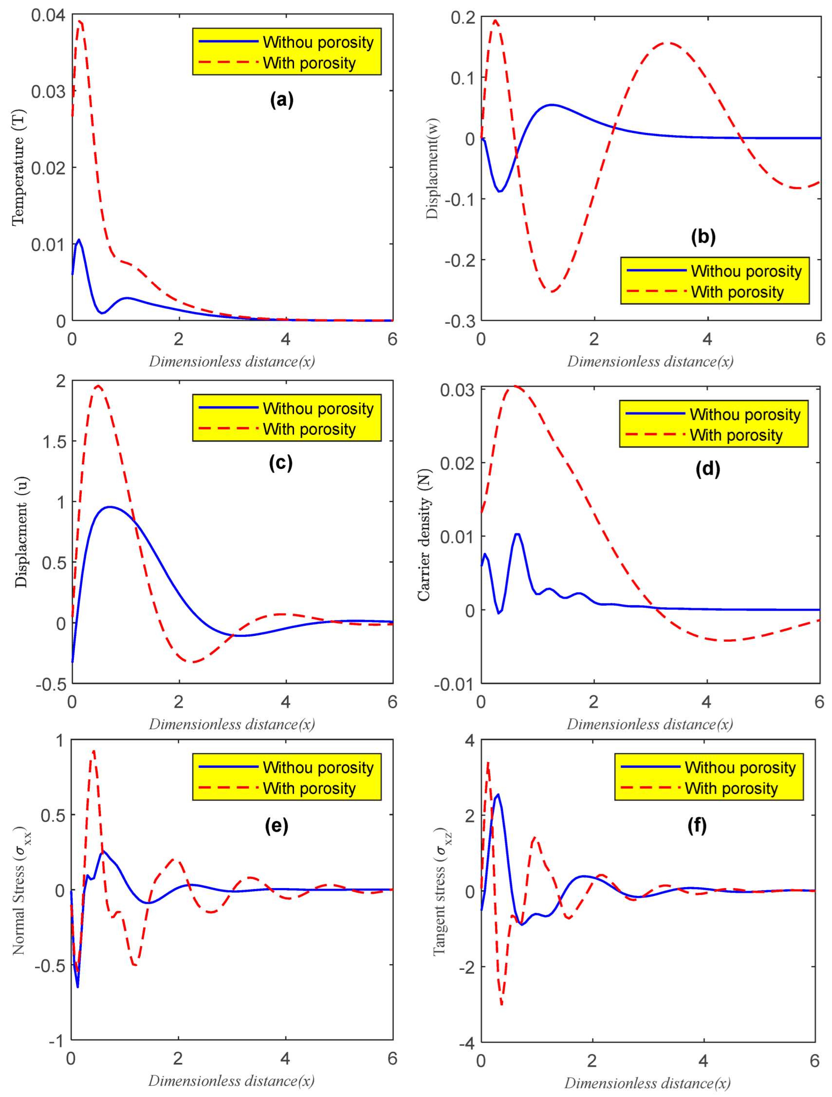
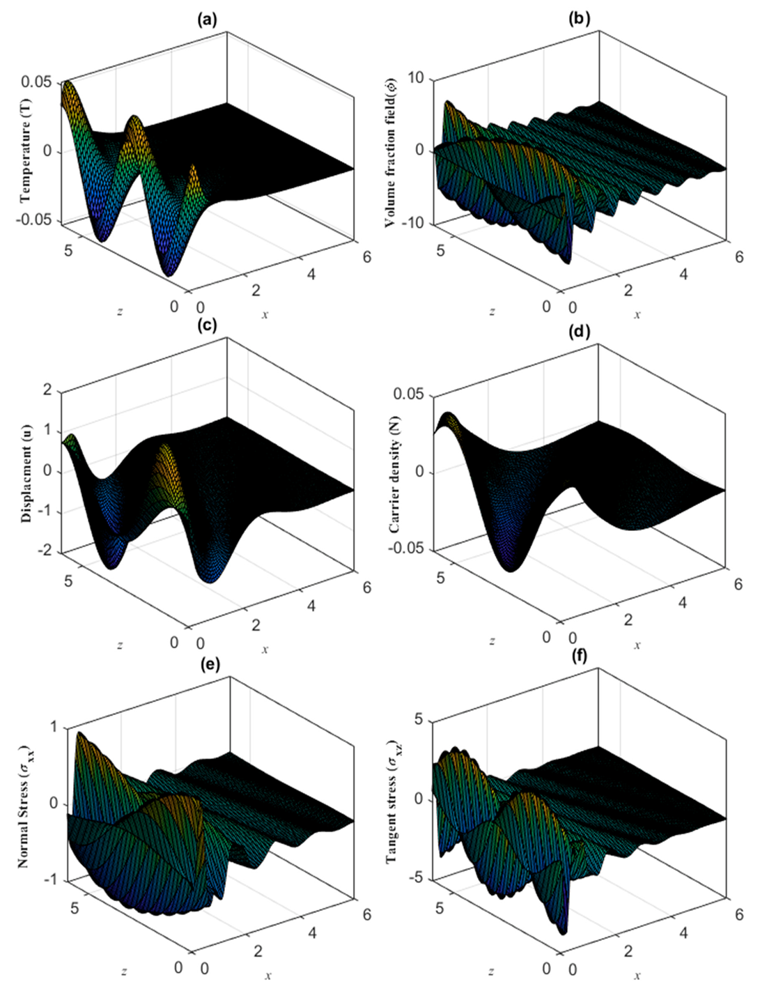
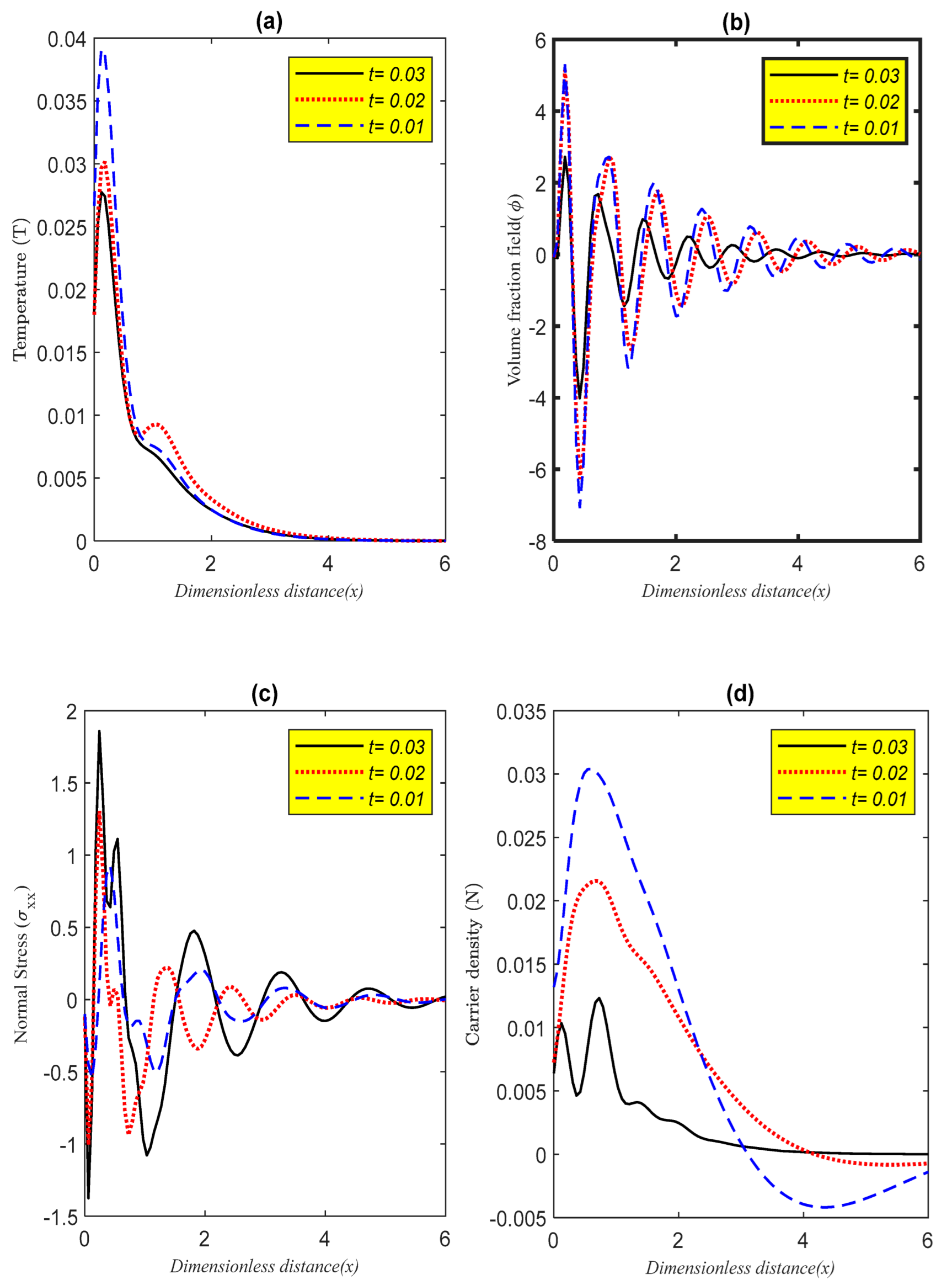
6. Numerical Results and Discussion

For use in numerical simulation, silicon (Si) component is an example of an elastic semiconductor material (using the MATLAB program). The numerical simulation and computational findings of fundamental quantity fields, which have various applications in contemporary industry and plasma physics technology, are performed using the physical constants of Si. For Si material (from n-type), the physical constants mentioned in

Table 1. The physical constants of Si (semiconductor) medium.

Unit	Symbol	Value	Unit	Symbol	Value
$N/m^2$	$\lambda$ $\mu$	$3.64\times {10}^{10}$ $5.46\times {10}^{10}$	$N$	$p$	$100$
$kg/m^3$	$\rho$	$2330\hspace{0.17em}$	$J/kg\hspace{0.17em}K$	$C_e$	$695\hspace{0.17em}$
$\mathrm{K}$	$T_0\hspace{1em}$	$800$	$\hspace{0.17em}\frac{m}{s}$	$\tilde{s}$	$2$
$s$	$\tau \hspace{0.17em}$	$5\times \hspace{0.17em}{10}^{-5}$	$m^2$	$\psi$	$1.753\hspace{0.17em}\times {10}^{-15}$
$m^3$	$d_n\hspace{0.17em}$	$-9\hspace{0.17em}\times \hspace{0.17em}{10}^{-31}$	$N$	$\alpha$	$3.688\hspace{0.17em}\times \hspace{0.17em}{10}^{-5}$
$m^2/s$	$D_E\hspace{0.17em}$	$2.5\times {10}^{-3}$	$N{m}^{-2}$	${\varsigma }_1$	$1.475\hspace{0.17em}\times \hspace{0.17em}{10}^{10}$
$eV$	$E_g\hspace{0.17em}$	$1.11$	$N{m}^{-2}$	${\lambda }_o$	$1.13849\hspace{0.17em}\times \hspace{0.17em}{10}^{10}$
$K^{-1}$	${\alpha }_t\hspace{0.17em}$	$4.14\hspace{0.17em}\times {10}^{-6}$	$N{m}^{-2}{\mathrm{deg}}^{-1}$	$m$	$2\times \hspace{0.17em}{10}^6$
$\hspace{0.17em}W{m}^{-1}{K}^{-1}$	$k\hspace{0.17em}$	$150\hspace{0.17em}$	$N{m}^{-2}{s}^{-1}$	${\omega }_o$	$0.0787\hspace{0.17em}\times \hspace{0.17em}{10}^{-3}$

as follows [33,34,35,36] are taken in SI units:

To create a numerical simulation for a brief period $t=0.001\hspace{0.17em}$ when the mechanical load is $\overline{P}=1$ in the range of $0\le x\le 6$ when $z=-1$, the non-dimensional main fields in 2D are created based on the Fourier–Laplace transform inversion approach. At the free surface of the semiconductor medium, the principal physical field propagates as a wave (transient) when boundary conditions (thermal, mechanical, and plasma conditions have an impact on all waves that are propagating) are taken into account. Wave propagation is significantly influenced by surface conditions. Figure 1 illustrates the primary physical distributions of temperature (thermal wave), the change in volume fraction field (volume fraction field), elastic wave (displacement), carrier charge density (plasma wave), and mechanical waves (${\sigma }_{xx}$ and ${\sigma }_{xz}$) with the horizontal distance following three models of the photo-thermoelasticity theory (CD, LS, and GL). The differences between the CD, LS, and GL models depend on the various thermal memories; all assessments are completed in a very short amount of time while taking into account the material constants of voids (pours) factors. All of the fields in this category (Figure 1 (from Figure 1a to Figure 1f) meet the requirements that are based on the semiconductor’s surface. During the electronic and thermoelastic deformation, the thermal wave (temperature, Figure 1a) and plasma wave (carrier density, Figure 1d) rise first (first range), then reach their maximum points. This is because of the thermal influence of the light beams. However, the thermal wave and plasma wave gradually decrease with exponential behavior for all three models in the second range, which is consistent with the experimental findings [37]. Starting at zero point at the surface, the volume fraction field distribution has a wave propagation rise near the surface due to the influence of light thermal to reach the maximum peak value for all three models. Due to the diminished thermal effect of light, it decreases fast in the second range to approach the minimum peak value inside the medium before increasing and decreasing periodically inside the semiconductor medium of the deceleration until it touches the zero line (the state of equilibrium). Due to increased vibrations of the material’s interior particles, the elastic wave (displacement component $u$, Figure 2c) starts at the initial surface value. It then grows quickly to achieve its highest maximum value (thermoelastic deformation) with wave propagated. As a result, to reach equilibrium, the elastic wave diminishes in the second range with exponential wave behavior until it crosses the zero line. There are two types of mechanical waves plotted: normal stress ${\sigma }_{xx}$ and tangent stress ${\sigma }_{xz}$. Due to the persistence in the electronic and elastic deformations, the normal stress distribution ${\sigma }_{xx}$ (Figure 1e) begins with a negative value at the surface and rapidly falls in the beginning to approach the peak minimum value close to the surface. To attain the peak maximum value in the second range, it grows abruptly. After that, it varies with wave behavior, regularly falling and rising until it reaches the equilibrium condition. The distribution of tangent stresses ${\sigma }_{xz}$ starts at zero and rises until it reaches its highest peak value in the first range. The second range, meanwhile, rapidly drops until it approaches the minimum peak value. It raises and drops regularly farther away from the surface until it achieves equilibrium by being congruent with the zero line.

Figure 2a–f shows the behavior of variation in the main physical fields with the horizontal distance according to two dimensionless cases: the first describes the wave propagations behavior without the porosity impact (when the porosity parameters are neglected), but the second case represents the wave propagations behavior under the influence porosity parameters. The GL model is used for all computations, which are performed for very short relaxation times under the influence of the photo-thermoelasticity hypothesis. Due to the effect of porosity, the values of the magnitude of wave propagations of the main fields are higher with porosity parameters than without porosity parameters. This figure shows that all wave propagations of the considered fields are significantly influenced by the porosity parameters. It has been found that porosity has a significant impact on how the main quantity distributions vary.

Figure 3 plots the dimensionless physical quantities for Si against the vertical ($0\le z\le 6$) and horizontal ($0\le x\le 6$) distances in three dimensions (3D). The computational outcomes are derived using the GL model under the influence of porosity parameters. According to this figure, changes in the vertical and horizontal distance have a significant influence on how waves propagate in all physical fields.

Figure 4 depicts the horizontal distance and various values of dimensionless time together with the wave propagation of the main field front distribution. All computations are made according to the GL model when the porosity effect is taken into account under the impact of initial stress. From this figure, it can be noticed that the thermal wavefront propagates faster than with the increase in dimensionless time.

7. Conclusions

A novel model of double porosity semiconductor material is investigated using the generalized thermoelasticity theory during photo-excitation transport processes. According to changes in thermal and elastic relaxation times, the governing equations are derived in two dimensions. The dimensionless main equations are solved according to the Laplace–Fourier techniques. Our discussion shows that when the horizontal distance increases, the wave distribution of all physical fields approaches the zero line to establish an equilibrium state. It has been discovered that every field quantity is extremely sensitive to the thermal relaxation time parameters according to the LS, GL, and CD models. The numerical simulations of the main fields make it clear that the porosity effect is significant. The graphic showed that the effects of double porosity on the numerical values of physical quantities were both increasing and decreasing. The boundary conditions applied to the surface have a significant impact on the semiconductor material’s tendency to deform again. The usage of this kind of research in solar cells, electric circuits, and sensors makes it beneficial. The outcomes of this study should be useful for those exploring the theory of photo-thermoelasticity based on the double porosity structure. A more realistic model is now available for further research thanks to the addition of the double porous parameter to the excited photo-thermoelastic material.

References

1. Lord, H.; Shulman, Y. A generalized dynamical theory of thermoelasticity. J. Mech. Phys. Solids 1967, 15, 299–309. [Google Scholar] [CrossRef]
2. Gordon, J.P.; Leite, R.C.C.; Moore, R.S.; Porto, S.P.S.; Whinnery, J.R. Long-transient effects in lasers with inserted liquid samples. Bull. Am. Phys. Soc. 1964, 119, 501–510. [Google Scholar] [CrossRef]
3. Kreuzer, L.B. Ultralow gas concentration infrared absorption spectroscopy. J. Appl. Phys. 1971, 42, 2934–2943. [Google Scholar] [CrossRef]
4. Mahdy, A.M.S.; Gepreel, K.A.; Lotfy Kh El-Bary, A.A. A numerical method for solving the Rubella ailment disease model. Int. J. Mod. Phys. C 2021, 32, 2150097. [Google Scholar] [CrossRef]
5. Todorović, D.M.; Nikolić, P.M.; Bojičić, A.I. Photoacoustic frequency transmission technique: Electronic deformation mechanism in semiconductors. J. Appl. Phys. 1999, 85, 7716–7726. [Google Scholar] [CrossRef]
6. Song, Y.; Todorovic, D.M.; Cretin, B.; Vairac, P. Study on the generalized thermoelastic vibration of the optically excited semiconducting microcantilevers. Int. J. Solids Struct. 2010, 47, 1871–1875. [Google Scholar] [CrossRef] [Green Version]
7. Abbas, I.A.; Alzahrani, F.S.; Elaiw, A. A DPL model of photothermal interaction in a semiconductor material. Waves Random Complex Media 2019, 29, 328–343. [Google Scholar] [CrossRef]
8. Khamis, A.K.; El-Bary, A.A.; Lotfy Kh Bakali, A. Photothermal excitation processes with refined multi dual phase-lags theory for semiconductor elastic medium. Alex. Eng. J. 2020, 59, 1–9. [Google Scholar] [CrossRef]
9. Hosseini, S.M.; Zhang, C. Plasma-affected photo-thermoelastic wave propagation in a semiconductor Love–Bishop nanorod using strain-gradient Moore–Gibson–Thompson theories. Thin-Walled Struct. 2022, 179, 109480. [Google Scholar] [CrossRef]
10. Hosseini, S.M.; Sladek, J.; Sladek, V. Nonlocal coupled photo-thermoelasticity analysis in a semiconducting micro/nano beam resonator subjected to plasma shock loading: A Green-Naghdi-based analytical solution. Appl. Math. Model. 2020, 88, 631–651. [Google Scholar] [CrossRef]
11. Nunziato, J.W.; Cowin, S.C. A non-linear theory of elastic materials with voids. Arch. Ration. Mech. Anal. 1979, 72, 175–201. [Google Scholar] [CrossRef]
12. Cowin, S.C.; Nunziato, J.W. Linear theory of elastic materials with voids. J. Elast. 1983, 13, 125–147. [Google Scholar] [CrossRef]
13. Dhaliwal, R.S.; Wang, J. Domain of influence theorem in the theory of elastic materials with voids. Int. J. Eng. Sci. 1994, 32, 1823–1828. [Google Scholar] [CrossRef]
14. Jhorar, R.; Tripathi, D.; Bhatti, M.M.; Ellahi, R. Electroosmosis modulated biomechanical transport through asymmetric microfluidics channel. Indian J. Phys. 2018, 92, 1229–1238. [Google Scholar] [CrossRef]
15. Bhatti, M.M.; Zeeshan, A.; Tripathi, D.; Ellahi, R. Thermally developed peristaltic propulsion of magnetic solid particles in biorheological fluids. Indian J. Phys. 2018, 92, 423–430. [Google Scholar] [CrossRef]
16. Ainouz, A. Homogenized double porosity models for poro-elastic media with interfacial flow barrier. Math. Bohem. 2011, 136, 357–365. [Google Scholar] [CrossRef]
17. Svanadze, M. External boundary value problems of steady vibrations in the theory of rigid bodies with a double porosity structure. Appl. Math. Mech. 2015, 15, 365–366. [Google Scholar] [CrossRef]
18. Straughan, B. Stability and uniqueness in double porosity elasticity. Int. J. Eng. Sci. 2013, 65, 1–8. [Google Scholar] [CrossRef]
19. Eringen, A.C. Microcontinuum Field Theories: I. Foundations and Solids; Springer: New York, NY, USA, 1999. [Google Scholar]
20. Ailawalia, P.; Singh, N. Effect of rotation in a generalized thermoelastic medium with hydrostatic initial stress subjected to ramp type heating and loading. Int. J. Thermophys. 2009, 30, 2078–2097. [Google Scholar] [CrossRef]
21. Abbas, I.A.; Kumar, R. Response of thermal source in initially stressed generalized thermoelastic half-space with voids, J. Comput. Theoret. Nanosci. 2014, 11, 1472–1479. [Google Scholar] [CrossRef]
22. Bachher, M.; Sarkr, N.; Lahiri, A. Generalized thermoelastic infinite medium with voids subjected to an instantaneous heat sources with fractional derivative heat transfer. Int. J. Mech. Sci. 2014, 89, 84–91. [Google Scholar] [CrossRef]
23. Bachher, M.; Sarkr, N.; Lahiri, A. Fractional order thermoelastic interactions in an infinite voids material due to distributed time-dependent heat sources. Meccanica 2015, 50, 2167–2178. [Google Scholar] [CrossRef]
24. Eringen, A.C. Linear theory of micropolar elasticity. J. Math. Mech. 1966, 15, 909–923. [Google Scholar]
25. Hobiny, A.; Abbas, I. A GN model on photothermal interactions in a two-dimensions semiconductor half space. Results Phys. 2019, 15, 102588. [Google Scholar] [CrossRef]
26. Marin, M.; Lupu, M. On harmonic vibrations in thermoelasticity of micropolar bodies. J. Vibrat. Control 1998, 4, 507–518. [Google Scholar] [CrossRef]
27. Green, A.E.; Lindsay, K.A. Thermoelasticity. J. Elast. 1972, 2, 507–518. [Google Scholar] [CrossRef]
28. Todorovic, D.M. Plasma, thermal, and elastic waves in semiconductors. Rev. Sci. Instrum. 2003, 74, 582–588. [Google Scholar] [CrossRef]
29. Tam, A.C. Applications of photoacoustic sensing techniques. Rev. Mod. Phys. 1986, 58, 381–389. [Google Scholar] [CrossRef]
30. Tam, A.C. Ultrasensitive Laser Spectroscopy; Academic Press: New York, NY, USA, 1983; pp. 1–108. [Google Scholar]
31. Tam, A.C. Photothermal Investigations in Solids and Fluids; Academic Press: Boston, MA, USA, 1989; pp. 1–33. [Google Scholar]
32. Honig, G.; Hirdes, U. A method for the numerical inversion of Laplace transforms. J. Comput. Appl. Math. 1984, 10, 113–132. [Google Scholar] [CrossRef] [Green Version]
33. Marin, M.; Stan, G. Weak solutions in Elasticity of dipolar bodies with stretch. Carpath. J. Math. 2013, 29, 33–40. [Google Scholar] [CrossRef]
34. Mandelis, A.; Nestoros, M.; Christofides, C. Thermoelectronic-wave coupling in laser photothermal theory of semiconductors at elevated temperatures. Opt. Eng. 1997, 36, 459–468. [Google Scholar] [CrossRef]
35. Hobiny, A.; Abbas, I. A study on photothermal waves in an unbounded semiconductor medium with cylindrical cavity. Mech. Time-Depend Mater. 2016, 6, 1–12. [Google Scholar] [CrossRef]
36. Lotfy Kh Hassan, W.; El-Bary, A.; Kadry, M. Response of electromagnetic and Thomson effect of semiconductor mediu due to laser pulses and thermal memories during photothermal excitation. Results Phys. 2020, 16, 102877. [Google Scholar] [CrossRef]
37. Liu, J.; Han, M.; Wang, R.; Xu, S.; Wang, X. Photothermal phenomenon: Extended ideas for thermophysical properties characterization. J. Appl. Phys. 2022, 131, 065107. [Google Scholar] [CrossRef]
Figure 1. (a–f) Variation of the main physical distributions w.r.t the distance for different relaxation times under the impact of porosity parameters.
Crystals 12 01603 g001
Figure 2. (a–f) Variation of the main physical distributions w.r.t the distance for different two cases of porosity under the impact of GL model.
Crystals 12 01603 g002
Figure 3. (a–f) Variation of the main physical distributions w.r.t the vertical and horizontal distance under the impact of porosity according to the GL model.
Crystals 12 01603 g003
Figure 4. (a–d) The main physical wave’s fronts distribution at different dimensionless time instants.
Crystals 12 01603 g004