Article

High-Throughput Computation of New Carbon Allotropes with Diverse Hybridization and Ultrahigh Hardness

1
Department of Mechanical Engineering, University of South Carolina, Columbia, SC 29208, USA
2
Hunan Key Laboratory for Micro-Nano Energy Materials and Device and School of Physics and Optoelectronics, Xiangtan University, Xiangtan 411105, China
*
Authors to whom correspondence should be addressed.
Crystals 2021, 11(7), 783; https://doi.org/10.3390/cryst11070783
Submission received: 31 May 2021 / Revised: 26 June 2021 / Accepted: 29 June 2021 / Published: 5 July 2021
(This article belongs to the Special Issue First-Principles SimulationNano-Theory)

Abstract

:
The discovery of new carbon allotropes with different building blocks and crystal symmetries has long been of great interest to broad materials science fields. Herein, we report several hundred new carbon allotropes predicted by the state-of-the-art RG 2 code and first-principles calculations. The types of new carbon allotropes that were identified in this work span pure sp 2 , hybrid sp 2 / sp 3 , and pure sp3 C–C bonding. All structures were globally optimized at the first-principles level. The thermodynamic stability of some selected carbon allotropes was further validated by computing their phonon dispersions. The predicted carbon allotropes possess a broad range of Vickers’ hardness. This wide range of Vickers’ hardness is explained in detail in terms of both atomic descriptors such as density, volume per atom, packing fraction, and local potential energy throughout the unit cell, and global descriptors such as elastic modulus, shear modulus, and bulk modulus, universal anisotropy, Pugh’s ratio, and Poisson’s ratio. For the first time, we found strong correlation between Vickers’ hardness and average local potentials in the unit cell. This work provides deep insight into the identification of novel carbon materials with high Vickers’ hardness for modern applications in which ultrahigh hardness is desired. Moreover, the local potential averaged over the entire unit cell of an atomic structure, an easy-to-evaluate atomic descriptor, could serve as a new atomic descriptor for efficient screening of the mechanical properties of unexplored structures in future high-throughput computing and artificial-intelligence-accelerated materials discovery methods.

1. Introduction

Carbon atoms can form several allotropes with different bond lengths due to their ability to from new and various hybridizations [1,2]. The three carbon allotropes that exist naturally are sp 2 , sp 3 , and hybrid sp 2 / sp 3 , which represent the following structures: graphite, diamond, and amorphous carbon, respectively. In the past few decades, there has been an intense amount of research into the fabrication of naturally existing carbon allotropes and new carbon allotropes with various hybridizations such as graphene, nanotubes, fullerenes, and lonsdaleite. Those new carbon allotropes can be materials with different dimensions; fullerenes are a zero-dimensional material (0D), carbon nanotubes are one-dimensional (1D), and graphene is a two-dimensional material (2D) [3,4,5,6,7,8,9,10]. Furthermore, more hybridizations have been predicted theoretically and synthesized experimentally, such as 1D sp-carbyne, 2D sp- sp 2 -graphyne, and 3D sp- sp 3 -yne-diamond [11,12]. Several techniques have been used to produce more carbon allotropes. Recently, graphite with sp 2 was transformed into a sp 2 / sp 3 mixture by cold compression at a pressure of 17 GPa, which produced a similar hardness to that of diamond [10]. This experimental discovery motivated researchers to fabricate more high-pressure carbon crystalline phases such as W-carbon [13], Z-carbon [14], M-carbon [5], O-carbon [15], and bct- C 4 carbon [7].
Superhard materials are desired in an enormous number of engineering applications, such as drilling and cutting tools, automotive and aerospace applications, medical implants, grinding and polishing, armor plating, and abrasives for lapping [16,17]. As a result, an extensive amount of research has been carried out on the enhancement and application of existing materials with high Vickers’ hardness, and with the goal to go beyond known materials to discover more novel materials with ultrahigh Vickers’ hardness values [16,17]. Discovering new superhard materials with Vickers’ hardness values greater than 40 GPa [18,19] requires an understanding the properties of those materials that explain why some materials are superhard, in order to make the process much simpler and screen out a huge number of untested materials from the large range of materials. In the past few years, there has been some effort to explain Vickers’ hardness through the development of theoretical and semiempirical models: (1) a thermodynamic concept that relates the chemical bonding to the energy density [20]; (2) the relationship of hardness with electronegativity and the electron holding energy of the bond [21]; (3) chemical bond strength [22]; (4) ionicity, charge density, and bond length [23]. When it comes to mathematically calculating Vickers’ hardness, Teter noted in 1998 that there is a correlation between shear modulus and Vickers’ hardness [24]. The equation that Teter used to define Vickers’ hardness is as follows:
H V , Teter = 0.151 G
where G is the shear modulus. Chen and his coworkers deduced that the discrepancy of Teter’s model with the experimental results is because Teter’s model does not consider plastic deformation in the model [25]. Chen suggested that Pugh’s ratio should be included in the Vicker’s hardness formula. Pugh’s ratio was defined as:
k = G B
where B is the bulk modulus. K is a measure of the brittleness of a material, i.e., high K arises in highly brittle materials. Chen’s model for Vickers’ hardness is given as follows:
H V , Chen = 2 ( k 2 G ) 0.585 3
Chen’s model yielded better results when it was compared to the experimental results. However, Tian in 2012 noticed that ductile materials such as KI and KCl had negative Vickers’ hardness values, since the intercept had a nonphysical basis [26]. As a result, Tian’s model was proposed. Tian’s model is defined as follows:
H V , Tian = 0.92 k 1.137 G 0.708
Tian’s model did not have an intercept term, which proved to be useful with ductile and brittle materials when compared with the experimental results. Therefore, Tian’s model was utilized in this work due to its massive success when compared to experimental results for a wide variety of ductile and brittle materials.
In this work, carbon allotropes were generated computationally utilizing a powerful code named RG 2 .   RG 2 code was used to generate carbon allotropes with different hybridizations. RG 2 code generates carbon allotropes with different hybridizations based on reasonable bonding features [27,28]. Some carbon allotropes generated by the code were also seen in SACADA database [29]. This demonstrates that the code is not only able to generate novel carbon allotropes, but also to reproduce some existing carbon allotropes, which proves the high proficiency of the code. The hybridization in the carbon allotropes, namely sp 2 , sp 3 , and hybrid sp 2 / sp 3 , can be judged by number of bonded neighbors (three, four, and mixed three and four, respectively) [30,31].

2. Computational Procedure and Methods

For generation and screening of materials, the following computational procedure was executed:
  • Step 1: Initially, the RG2 code generated 1598 carbon allotropes in total with different hybridization states.
  • Step 2: We perform first-principles calculations to fully optimize those structures with low Monkhorst-pack k-mesh. The k-mesh in low-resolution DFT calculations depends on total number of atoms in the cell. Specifically, for numbers of atoms < 10 , 11 30 , 30 50 , and > 50 , the k-mesh was 8 × 8 × 8 , 4 × 4 × 4 , 2 × 2 × 2 , and 1 × 1 × 1 , respectively. After this step, we had 1576 carbon allotropes.
  • Step 3: We continued to perform first-principles calculations to fully optimize the structures that were successfully optimized in the previous step, with high Monkhorst-pack k-mesh. The k-mesh in high-resolution DFT calculations depends on the length of lattice of the cell. Specifically, the product of the k-mesh in each direction and lattice size was approximately 60 Å. This was equivalent to the k-mesh of 16 × 16 × 16 for diamond with an 8-atom conventional cell, which was high enough for global structure optimization. After this step, we had 1461 carbon allotropes.
  • Step 4: After global structure optimization was finished, we cross-checked the 1461 carbon structures and also compared the structures with those downloaded from the SACADA database [29]. We found that some of the finally optimized structures had been already identified or reported in previous studies. After cross-checking and screening, we had 1105 new and unique carbon allotropes.
  • Step 5: We finally calculated the elastic constants with conventional unit cells for all 1105 unique structures. Again, the k-mesh in each direction was determined by the same procedure as in Step 3. After this step, we successfully obtained the elastic constants of 1105 carbon allotropes.
  • Step 6: Some structures had unreasonable universal anisotropy [32] so we decided to only report the carbon allotropes with universal anisotropy between 0 and 3. Finally, 904 carbon allotropes remained from all the screening processes.
The RG 2 package was used to generate new carbon structures in which sp 2 , sp3, and sp 2 / sp 3 mixture hybridizations were formed [28,33,34,35]. The input parameters of RG2 mainly included the target space symmetry group(s), elements, number of inequivalent atoms in the unit cell, number of bonded atoms for each element, and bond feature information (e.g., bond angle, bond length, and the tolerance for their derivation). With these input parameters, the RG2 package built the correct labeled quotient graph. In this article, different structures with different numbers of carbon structures with different hybridization states were arbitrarily distributed in a stochastic cell which had an arbitrary symmetry and lattice constant [27]. The number of symmetrically independent atoms usually ranged from 2 to 10, with majority between 3 and 7. A structure was initially generated with an equivalent number of carbon atoms based on symmetry. The code then computed the distance matrix of all the carbon atoms in that specifically generated structure and built the labeled quotient graph (LQG) based on sp 2 or sp 3 hybridizations. The generated structures with reasonable LQGs based on the bond lengths and angles could be relaxed by the code. The new structures produced by the code were named according to parameters used to predict the structures in the code, and those parameters (characters or numbers) used in the names were separated by a hyphen. The naming process took place from left to right as the following: space group number, number of nonequivalent atoms in the unit cells, element names (always C in this work), ring or loop structure in carbon local ID, and possibly one more hyphen to distinguish two IDs.
Vienna ab initio simulation package (VASP) was used to perform first-principles calculations based on the density functional theory (DFT) [36,37,38]. Global structure optimization was carried out in VASP with full degrees of freedom for both lattice shape, size, and atomic coordinates. As for the exchange-correlation functional, the Perdew–Burke–Ernzerhof (PBE) generalized gradient approximation (GGA) was selected [39]. The kinetic energy cutoff for the electronic wavefunctions was set to be 520 eV with a plane-wave basis set obtained through projector augmented wave method (PAW) modeling [38,40]. The value of 520 eV was chosen by following the recommendation from VASP, i.e., the energy cutoff should be at least 1.3 times the maximum ENMAX for an atomic species in a material, which is equal to 400 eV for carbon. Different Monkhorst-pack k-mesh sizes were used depending on the lattice constants to sample the Brillouin zone [41]. Generally speaking, the k-mesh size used was dense enough and equivalent to a regular diamond lattice (primitive cell) at 16 × 16 × 16. The energy and force criteria for the structure optimization were 10 7   eV and 10 4   eV / A , respectively. The unit cell could change its size, and the atoms could move to reach the convergence criteria mentioned previously.
The elastic stiffness tensor matrix was calculated via the finite difference method in VASP by the conventional unit cell constructed with the relaxed structure from the structure optimization process. The elastic stiffness tensor was obtained from the OUTCAR file, which is an output file from running VASP code with Hessian matrix calculations from finite differences. The Hessian matrix is the matrix of the second derivatives of energy with respect to the positions of atoms, which is also used to compute the elastic stiffness tensor in VASP. The elastic stiffness tensor matrix can be obtained by executing six finite distortions on the unit cell/lattice and deriving the elastic constants from the stress–strain relationship [42]. For each crystal system, the elastic stiffness tensor matrix is different [43]. The most general form, which is also applied to the triclinic crystal system, is shown below:
C = [ c 11 c 12 c 13 c 14 c 15 c 16 c 21 c 22 c 23 c 24 c 25 c 26 c 31 c 32 c 33 c 34 c 35 c 36 c 41 c 42 c 43 c 44 c 45 c 46 c 51 c 52 c 53 c 54 c 55 c 56 c 61 c 62 c 63 c 64 c 65 c 66 ]
where c i j is the elastic constant component in direction ij and c i j = c j i . The number of independent elastic constants varies for each crystal system depending on the symmetry of the crystal system. For example, the triclinic crystal system, which is the least symmetrical crystal system, has 21 independent elastic constants, whereas a cubic crystal system, which is the most symmetrical crystal system, only has three independent elastic constants. It can be noted that the crystal system in the most general form in Equation (5) is triclinic with 21 independent elastic constants, assuming that all the elastic constants are independent. Some of the elastic constants can be equal to zero. Also, some elastic constants in certain directions can be equal to elastic constants in other directions which means that those elastic constants are dependent. All the previously mentioned two different scenarios related to elastic constants can be represented in a cubic crystal system as
c c u b i c = [ c 11 c 12 c 12 0 0 0 c 12 c 11 c 12 0 0 0 c 12 c 12 c 11 0 0 0 0 0 0 c 44 0 0 0 0 0 0 c 44 0 0 0 0 0 0 c 44 ]
In Equation (6), some elastic constants in the cubic crystal system are dependent in which c 12 = c 13 , c 11 = c 22 = c 33 , and c 44 = c 55 = c 66 . Moreover, many of the elastic constants in the elastic stiffness tensor matrix are equal to zero. The compliance tensor is the inverse of the elastic tensor and defined as
[ c i j ] = [ s i j ] 1
Shear ( G ) and bulk ( B ) moduli calculations from the elastic constants can be calculated through two definitions averaging Viogt’s [44] approximation and Reuss’ [45] approximation. Voigt’s approximation assumes uniform strain throughout the crystal, while Reuss’ approximation assumes uniform stress throughout the crystal. The Voigt’s bound equations take the following form:
9 B V = ( c 11 + c 22 + c 33 ) + 2 ( c 12 + c 23 + c 31 ) 15 G V = ( c 11 + c 22 + c 33 ) ( c 12 + c 23 + c 31 ) + 4 ( c 44 + c 55 + c 66 )
where as the Reuss’ equations are:
1 B R = ( s 11 + s 22 + s 33 ) + 2 ( s 12 + s 23 + s 31 ) 15 / G R = 4 ( s 11 + s 22 + s 33 ) 4 ( s 12 + s 23 + s 31 ) + 3 ( s 44 + s 55 + s 66 )
Hill demonstrated that both Reuss and Voigt approximations are strictly lower and upper bounds, and the average of both approximations yields the actual elastic behavior results for G and B in polycrystalline materials [46]. Therefore, G and B according to Hill are as follows:
B V R H = ( B V + B R ) 2 G V R H = ( G V + G R ) 2
In this article, Hill’s approximation is implemented for G and B in the Results and Discussion section.
Young’s modulus and Poisson’s ratio are defined as follows:
E = 9 B G 3 B + G
ν = 3 B 2 G 2 ( 3 B + G )
Researchers have made a significant effort to quantify anisotropy. In 1948, Zener introduced a definition to quantify anisotropy in which he used the elastic constants c 11 , c 12 , and c 44 from the elastic stiffness tensor, and the formula A = 2 c 44 c 11 c 12 [47]. In 1967, Chung proposed another empirical formula to measure the anisotropy of cubic crystal systems in which he utilized the Voigt and Reuss approximations in the formula [48]. Chung’s definition was A c = G V G R G V + G R . The previous two definitions of anisotropy have a good performance to a certain extent since they yield acceptable results when it comes to cubic crystals, which have an isotropic bulk resistance. However, the definitions do not show adequate results when they are used in other crystal systems besides the cubic crystal system, because the other systems generally exhibit anisotropic bulk resistance responses. In order to accurately quantify anisotropy, all the contributions must be considered. To this end, Ranganathan proposed a novel formula to quantify universal anisotropy which overcame the constraints of the two previous definitions [32]. The formula of universal anisotropy is
A U = 5 G V G R + B V B R 6
In this work, the universal anisotropy definition from Ranganatha is implemented in the Results and Discussion section.
A supercomputer with 48 cores per node was used. All VASP jobs were run on 24 cores, i.e., one node could run two VASP jobs simultaneously. Generally speaking, the CPU time for optimization of a carbon structure ranged from a few minutes to several hours, depending on the systems, with majority around half an hour, while the elastic constant calculation typically took 1 to 5 h per structure.
A supercell of 2 × 2 × 2 of four carbon allotropes (their crystal structures are shown in Figure 1 and their IDs with their materials properties are in Table 1 in the Results and Discussion section) were created. The harmonic second-order force constant for those four materials was obtained via the finite displacement method using PHONOPY code [49]. Using PHONOPY code, the dynamic matrix of the reciprocal space was obtained from the energy derivatives to plot the phonon dispersion of each carbon allotrope.

3. Results and Discussion

The RG 2 code originally generated 1598 carbon allotropes, from which 1576 carbon allotropes were successfully optimized with low resolution. Subsequently, 1461 carbon allotropes were optimized with a high resolution of 16×16×16. Some structures already existed in SACADA database or had been reported in previous studies [29], but 1105 unique carbon allotropes remained after screening the 1461 carbon allotropes from those that already existed in SACADA. Some carbon allotropes exhibited high universal anisotropy [32], so carbon allotropes with universal anisotropy between 0 and 3 remained. After multiple screening steps, 904 carbon allotropes with different hybridization states remained from the RG 2 code. A total of 309 carbon allotropes had Vickers’ hardness values from Tian’s model greater than 40 GPa, which qualified them as superhard materials [18,19]. The structural information and the mechanical properties for all new carbon allotropes reported herein are provided as a separate JSON file as supplemental material. Mechanical properties such as shear modulus ( G ), bulk modulus ( B ), Poisson’s ratio ( ν ), Pugh’s ratio ( k ), elastic modulus ( E ), and Vickers’ hardness ( H ) using Tian’s model were calculated using the elastic constants in the elastic stiffness tensor matrix from the OUTCAR file outputted by VASP, and the structural properties such as density (ρ), volume per atom (VPA), and packing fraction (PF) were calculated using Matminer [50]. Average local potential (defined below) was also calculated from the LOCPOT file outputted by VASP to analyze the average atomic interactions in the unit cell. Positive values of local potential indicate repulsive interactions and, as local potential gets higher, interactions become more repulsive. On the other hand, negative local potential represents attraction and, the more negative the potential, the more attraction is present between the atoms [51,52].
V L O C P O T ( r ) = V ( r ) + n ( r ) | r r | d r + V X C ( r )

3.1. Ground-State Energy and Thermodynamic Stability

Figure 1 shows the 2 × 2 unit cells of selected carbon allotropes with different hybridizations, in which VESTA code was used for plotting [53]. The materials with their hybridizations are (a) 135-3-40-C-r89-np-id355667 with pure sp 2 bonding, (b) 136-3-20-C-r689-np-id545421_1 with hybrid sp 2 / sp 3 bonding, (c) 179-3-36-C-r6789-p-id545421 with pure sp 3 bonding, and (d) 165-3-28-C-r68-np-id545421 with pure sp 3 . The atomic structures of the carbon allotropes mentioned previously are shown in Figure 1.
Figure 2 shows their corresponding phonon dispersion for each selected carbon allotrope in Figure 1.
The phonon dispersions of each structure (shown in Figure 2) indicated that all the structures were thermodynamically stable since no negative phonon frequency was found in the phonon dispersion plots [54,55,56,57], which means that those carbon allotropes could be synthesized experimentally [58]. Interestingly, the acoustic phonon dispersions show in Figure 2c had few couplings or intersection with optical phonons until 10 THz. This feature is very promising for high thermal conductivity of this structure, since the intrinsic acoustic–optical phonon scattering would be very weak. The ground-state energy per atom for the final unique 904 carbon allotropes ranged from 9.2795   eV / atom to 7.6504   eV / atom . Many new structures had energy values very close to that of diamond, which is 9.0929   eV / atom . It is worth noting that, although the carbon allotropes were similar in the sense that they only contained the single element of carbon, these carbon allotropes were different and displayed a wide range of various properties, which was also confirmed by the diverse mechanical properties and ground-state energy calculations. Table 1 shows a summary of important information about the four representative structures with their Vickers’ hardness results.
From Table 1, it can be noted that both materials with pure sp 3 hybridizations had higher Vickers’ hardness values than the other two hybridizations. The structure with pure sp 2 had the lowest Vickers’ hardness. The hybridization sp 3 was noted to have higher Vickers’ hardness for the available data used in this article. The area occupied by materials with sp 3 and sp 2 hybridizations in a 2D map of shear and bulk moduli with Pugh’s ratio and Poisson’s ratio as indicators for high and low hardness is shown below.

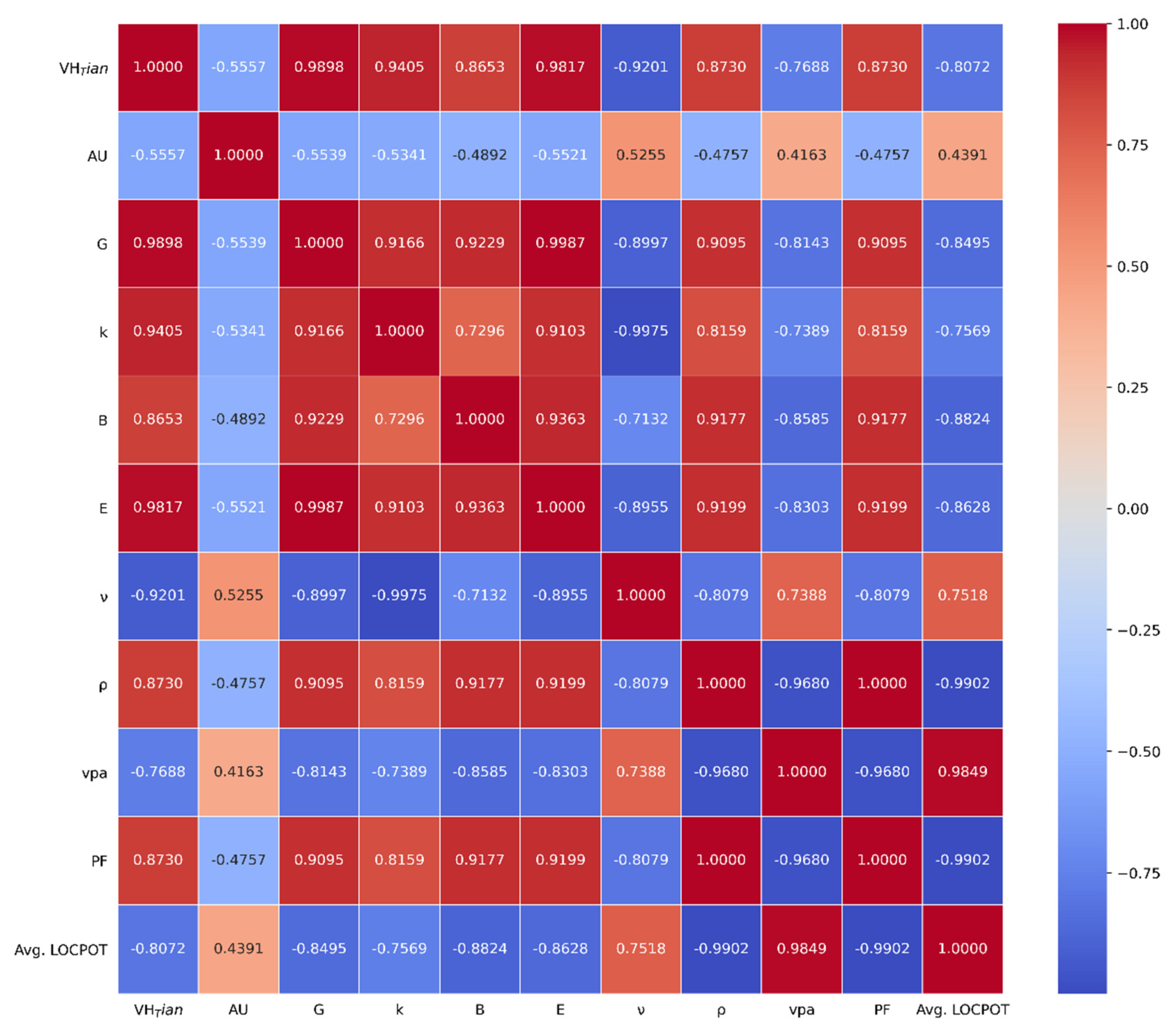
3.2. Pearson Correlation

The Pearson correlation matrix of the properties mentioned previously is shown in Figure 3. The Pearson correlation matrix was generated using open-source Python to give an insight of how much each property correlated with the other properties [59]. Since the explanation of Vickers’ hardness is more important in this article than explaining the other properties, the Vickers’ hardness explanation based on the other properties is the focus.
A Pearson correlation matrix relates two parameters to each other, and the values are between −1 and 1. A value of −1 in the correlation matrix indicates a perfectly inverse correlation between two parameters, a value of 0 indicates that no correlation exists between the two parameters, and a value of 1 indicates a perfect positive correlation. If a value is between 0 and 1, the correlation is direct, and the degree of the direct correlation depends on the value itself. If the value is close to 0, that denotes a weak direct correlation. Furthermore, if the value is close to 1, a strong direct correlation is present between two parameters. The same explanation applies to the numbers between −1 and 0, wherein a weak inverse correlation exists if the value is close to 0, but a strong inverse correlation exists between two forms of criteria if the value is close to −1. In Figure 3, values of 1 are present in the diagonal elements of the matrix, which is because the column and row parameters are identical. For example, the third row in the correlation matrix is shear modulus ( G ) and the third column is shear modulus ( G ), so it makes sense that the correlation between them is equal to 1 because they are identical. The properties that were directly proportional to Vickers’ hardness were shear modulus, bulk modulus, elastic modulus, Pugh’s ratio, density, and packing fraction. The properties that were inversely proportional to Vickers’ hardness are universal anisotropy, Poisson’s ratio, volume per atom, and average local potential. Table 2 shows some carbon allotropes with high hardness. Table 3 shows some carbon allotropes with low hardness.
The Pearson correlation confirmed some results in the literature that we mentioned previously, and showed some obvious correlations with Vickers’ hardness. Pugh’s ratio and shear modulus are part of the Vickers’ hardness definition in Equation (4), so it is obvious why the correlation between Vickers’ hardness with Pugh’s ratio and Vickers’ hardness with shear modulus was extremely high. However, some properties are not included in Equation (4), but they were highly proportional to Vickers’ hardness. Bulk modulus was highly correlated with hardness, and it has been reported in the literature that a linear correlation between hardness and bulk modulus could be used to calculate hardness in InSb, GaSb, Ge, Si, and diamond, but failed in a wide range of other materials [60,61]. It has also been reported that the relationship between hardness and bulk modulus is nonlinear and cannot be used to calculate hardness in many different types of materials [24,62]. The Pearson correlation shown in Figure 3 suggests that the correlation between hardness and bulk modulus was 0.8653, which is high, but not as high as the shear modulus and Pugh’s ratio correlation coefficients (0.9898 and 0.9405, respectively). Tian reported that materials with high hardness tend to have a high elastic modulus [26]. Figure 3 and the comparison between Table 2 and Table 3 confirms Tian’s report, with an exceptionally high correlation coefficient of 0.9817 which also happened to be even higher than the correlation coefficient of shear modulus with Vickers’ hardness, which was equal to 0.9405.
Volume per atom, density, and packing fraction results from Figure 3 and Table 2 and Table 3 indicated that materials with high Vickers’ hardness are more packed and denser than materials with lower Vickers’ hardness. Local potential differs from one area to another in a unit cell since electrons and nuclei are in different positions throughout the unit cell, which consequently affects the value of local potential in each grid of the unit cell. We believe that the average local potential of the unit cell gives a massive insight into the interactions of the unit cell, as proven by the results from Figure 3 and Table 2 and Table 3. The Pearson correlation shown in Figure 3 indicates that the relationship between local potential and hardness had a correlation coefficient of −0.8072. In other words, materials with lower local potential in their unit cells have high hardness. This can be interpreted by the fact a high attraction of unit cells with lower local potential occurs in materials with high hardness, which also reflects the high strength in the bonds of those materials. Table 2 confirms that materials with high hardness had local potentials lower than −13 eV (i.e., higher attraction) whereas the materials with low hardness shown in Table 3 had local potentials higher than −9 eV (i.e., lower attraction). The higher attraction with lower local potential in superhard materials also explains why the superhard carbon allotropes had high density and packing fraction.
It was also noted that a strong inverse relationship occurred between Poisson’s ratio and Vickers’ hardness (−0.9201). This result confirms that ductile/brittle materials have low/high hardness, since high/low Poisson’s ratio is an indicator of a ductile/brittle material [63]. The Pearson correlation matrix in Figure 3 also shows that highly anisotropic materials had lower hardness and vice versa, which was also confirmed by the comparison between the superhard materials shown in Table 2 with the materials with low Vickers’ hardness shown in Table 3. Poisson’s and Pugh’s ratios had an extraordinarily high inverse correlation with a coefficient of −0.9975 from Pearson correlation matrix, as shown in Figure 3, and both Pugh’s and Poisson’s ratios also had an extremely correlation with Vickers’ hardness of the carbon allotropes (as shown in Figure 3). In fact, they are mathematically related by combining Equations (2) and (12) to yield the following equation [64]:
ν = 3 2 k 2 ( 3 + k ) = 3 2 k 6 + 2 k
Equation (15) also confirms the inverse correlation between Pugh’s ratio and Poisson’s ratio because when k gets larger, ν gets smaller, and vice versa. Furthermore, Pugh’s and Poisson’s ratios have inverse physical interpretations, and both are used to classify brittle and ductile materials. Materials with high Pugh’s ratio (> 0.57) and small Poisson’s ratio (< 0.33) are brittle materials [63], and vice versa.
Figure 4 and Figure 5 show the relationship of shear and bulk moduli with Pugh’s ratio and Poisson’s ratio, respectively. Figure 4 and Figure 5 visually explain hardness using the 2D map of bulk modulus vs. shear modulus and show Pugh’s ratio and Poisson’s ratio, which are strongly correlated to Vickers’ hardness, as color bars. Carbon allotropes with high hardness had high bulk and shear moduli, as shown previously in Figure 3 and Table 2 and Table 3.
It is shown in Figure 4 and Figure 5 that Pugh’s ratio changed with different bulk and shear moduli values. Where the shear modulus was equal to 200 GPa, different colors of Pugh’s ratio and different values of bulk modulus appear in Figure 4. Therefore, hardness differed among different materials with the same value of shear modulus. Furthermore, the materials with higher values of shear modulus with the same value of bulk modulus had higher Pugh’s ratios and consequently higher Vickers’ hardness. Carbon allotropes with pure sp 3 hybridization had a high Pugh’s ratio, bulk modulus, and shear modulus, so they are shown in the upper right area of Figure 4. On the other hand, carbon allotropes with pure sp 2 hybridization had lower Pugh’s ratio, bulk modulus, and shear modulus, which means that they are shown at the lower left of Figure 4. As for hybrid sp 2 / sp 3 , it had a wide range of Vickers’ hardness values, and the materials with hybrid sp 2 / sp 3 bonding are placed between pure sp 2 and pure sp 3 in Figure 4.
It is shown in Figure 4 and that Pugh’s ratio and Poisson’s ratio changed with different bulk and shear moduli. When the bulk modulus was equal to 200 GPa, shear modulus and Poisson’s ratio differed in those carbon allotropes (Figure 5), and the carbon allotropes with higher shear modulus with the same bulk modulus had lower Poisson’s ratio and higher Vickers’ hardness. Carbon allotropes with pure sp 2 , hybrid sp 2 / sp 3 , and pure sp 3 had the same positions in Figure 5 as in Figure 4 even after the color bar was changed from Pugh’s ratio in Figure 4 to Poisson’s ratio in Figure 5. Figure 4 and Figure 5 also confirm the inverse relationship between Poisson’s ratio and Pugh’s ratio shown in the Pearson correlation in Figure 3.

4. Conclusions

Discovering new materials has been an important research topic in the past few decades. In this report, the state-of-the-art RG 2 predicted new carbon allotropes that had ultrahigh hardness (40 GPa) according to Tian’s model, which has been shown to be successful in calculating Vickers’ hardness values for a wide variety of ductile and brittle materials. Those new carbon allotropes had a wide range of hybridizations, including pure sp 2 , hybrid sp 2 / sp 3 , and pure sp3. First-principles calculations were performed to optimize the structures and calculate Vickers’ hardness. Atomic descriptors such as packing fraction, density, and volume per atom along with mechanical properties such as bulk, shear, and elastic moduli; universal anisotropy; Poisson’s ratio; and Pugh’s ratio were utilized to explain the wide range of Vickers’ hardness results for the ductile and brittle carbon allotropes. The relationships between the average of local potential in the carbon allotrope unit cell and the anisotropy of a carbon allotrope with Vickers’ hardness were reported for the first time in this article, to the best of our knowledge. We believe that this work adds more insight and understanding to Vickers’ hardness in terms of finding various descriptors to explain Vickers’ hardness and accelerating the process of discovering unexplored novel superhard materials with captivating properties.

Supplementary Materials

The following are available online at https://www.mdpi.com/article/10.3390/cryst11070783/s1, JSON file: The structural infor-mation and the mechanical properties for all reported new carbon allotropes.

Author Contributions

Conceptualization, M.H.; methodology, M.A.-F., T.O.; software, T.O.; validation, T.O. and M.H.; analysis, M.A.-F., A.R.; investigation, M.A.-F., A.R.; data curation, M.A.-F., T.O. and M.H.; writing—original draft preparation, M.A.-F.; writing—review and editing, M.A.-F., T.O., M.H.; supervision, M.H.; project administration, M.H.; funding acquisition, T.O., M.H. All authors have read and agreed to the published version of the manuscript.

Funding

This research was funded by NASA SC Space Grant Consortium REAP Program (Award No.: 521179-RP-SC005) and Scientific Research Fund of Hunan Provincial Education Department (No. 20K127).

Data Availability Statement

The data presented in this study are available in Supplementary Material.

Acknowledgments

This research is partially supported by the NASA SC Space Grant Consortium REAP Program (Award No.: 521179-RP-SC005). T.O. acknowledges Scientific Research Fund of Hunan Provincial Education Department (No. 20K127).

Conflicts of Interest

The authors declare no conflict of interest.

References

  1. Zhao, Z.; Xu, B.; Wang, L.-M.; Zhou, X.-F.; He, J.; Liu, Z.; Wang, H.-T.; Tian, Y. Three dimensional carbon-nanotube polymers. ACS Nano 2011, 5, 7226–7234. [Google Scholar] [CrossRef]
  2. Miller, E.D.; Nesting, A.D.C.; Badding, J. Quenchable transparent phase of carbon. Chem. Mater. 1997, 9, 18–22. [Google Scholar] [CrossRef]
  3. Wang, Z.; Zhao, Y.; Tait, K.; Liao, X.; Schiferl, D.; Zha, C.; Downs, R.T.; Qian, J.; Zhu, Y.; Shen, T. A quenchable superhard carbon phase synthesized by cold compression of carbon nanotubes. Proc. Natl. Acad. Sci. USA 2004, 101, 13699–13702. [Google Scholar] [CrossRef] [Green Version]
  4. Ivanovskaya, V.V.; Ivanovskii, A.L. Simulation of novel superhard carbon materials based on fullerenes and nanotubes. J. Superhard Mater. 2010, 32, 67–87. [Google Scholar] [CrossRef]
  5. Li, Q.; Ma, Y.; Oganov, A.R.; Wang, H.; Wang, H.; Xu, Y.; Cui, T.; Mao, H.-K.; Zou, G. Superhard monoclinic polymorph of carbon. Phys. Rev. Lett. 2009, 102, 175506. [Google Scholar] [CrossRef] [Green Version]
  6. Sheng, X.-L.; Yan, Q.-B.; Ye, F.; Zheng, Q.-R.; Su, G. T-Carbon: A novel carbon allotrope. Phys. Rev. Lett. 2011, 106, 155703. [Google Scholar] [CrossRef] [Green Version]
  7. Umemoto, K.; Wentzcovitch, R.M.; Saito, S.; Miyake, T. Body-centered tetragonal C4: A viable sp3 carbon allotrope. Phys. Rev. Lett. 2010, 104, 125504. [Google Scholar] [CrossRef]
  8. Zhou, X.-F.; Qian, G.-R.; Dong, X.; Zhang, L.; Tian, Y.; Wang, H.-T. Ab initio study of the formation of transparent carbon under pressure. Phys. Rev. B 2010, 82, 134126. [Google Scholar] [CrossRef] [Green Version]
  9. Zhu, Q.; Oganov, A.R.; Salvadó, A.M.; Pertierra, P.; Lyakhov, A.O. Denser than diamond: Ab initio search for superdense carbon allotropes. Phys. Rev. B 2011, 83, 193410. [Google Scholar] [CrossRef] [Green Version]
  10. Mao, W.L.; Mao, H.-K.; Eng, P.J.; Trainor, T.P.; Newville, M.; Kao, C.-C.; Heinz, D.L.; Shu, J.; Meng, Y.; Hemley, R.J. Bonding changes in compressed superhard graphite. Science 2003, 302, 425–427. [Google Scholar] [CrossRef] [PubMed] [Green Version]
  11. Diederich, F.; Kivala, M. All-carbon scaffolds by rational design. Adv. Mater. 2010, 22, 803–812. [Google Scholar] [CrossRef] [PubMed]
  12. Hirsch, A. The era of carbon allotropes. Nat. Mater. 2010, 9, 868–871. [Google Scholar] [CrossRef] [PubMed]
  13. Wang, J.T.; Chen, C.F.; Kawazoe, Y. Low-temperature phase transformation from graphite to sp3 orthorhombic carbon. Phys. Rev. Lett. 2011, 106, 075501. [Google Scholar] [CrossRef] [PubMed] [Green Version]
  14. Zhao, Z.; Xu, B.; Zhou, X.; Wang, L.-M.; Wen, B.; He, J.; Liu, Z.; Wang, H.-T.; Tian, Y. Novel superhard carbon: C-centered orthorhombic C8. Phys. Rev. Lett. 2011, 107, 215502. [Google Scholar] [CrossRef] [PubMed]
  15. Wang, J.T.; Chen, C.F.; Kawazoe, Y. Orthorhombic carbon allotrope of compressed graphite: Ab initio calculations. Phys. Rev. B 2012, 85, 033410. [Google Scholar] [CrossRef] [Green Version]
  16. Kanyanta, V. Hard, superhard and ultrahard materials: An overview. In Microstructure-Property Correlations for Hard, Superhard, and Ultrahard Materials; Springer: Berlin/Heidelberg, Germany, 2016; pp. 1–23. [Google Scholar]
  17. Tehrani, A.M.; Brgoch, J. Hard and superhard materials: A computational perspective. J. Solid State Chem. 2019, 271, 47–58. [Google Scholar] [CrossRef]
  18. Haines, J.; Leger, J.M.; Bocquillon, G. Synthesis and design of superhard materials. Annu. Rev. Mater. Res. 2001, 31, 1–23. [Google Scholar] [CrossRef]
  19. Vepřek, S. Nanostructured superhard materials. In Handbook of Ceramic Hard Materials; Riedel, R., Ed.; Wiley: Weinheim, Germany, 2000; p. 109. [Google Scholar]
  20. Mukhanov, V.A.; Kurakevych, O.O.; Solozhenko, V.L. Thermodynamic model of hardness: Particular case of boron-rich solids. J. Superhard Mater. 2010, 32, 167–176. [Google Scholar] [CrossRef]
  21. Li, K.; Wang, X.; Zhang, F.; Xue, D. Electronegativity identification of novel superhard materials. Phys. Rev. Lett. 2008, 100, 235504. [Google Scholar] [CrossRef]
  22. Šimůnek, A.; Vackář, J. Hardness of covalent and ionic crystals: First-principle calculations. Phys. Rev. Lett. 2006, 96, 085501. [Google Scholar] [CrossRef] [Green Version]
  23. Gao, F.; He, J.; Wu, E.; Liu, S.; Yu, D.; Li, D.; Zhang, S.; Tian, Y. Hardness of covalent crystals. Phys. Rev. Lett. 2003, 91, 015502. [Google Scholar] [CrossRef] [PubMed]
  24. Teter, D.M. Computational alchemy: The search for new superhard materials. MRS Bull. 1998, 23, 22–27. [Google Scholar] [CrossRef]
  25. Chen, X.-Q.; Niu, H.; Li, D.; Li, Y. Modeling hardness of polycrystalline materials and bulk metallic glasses. Intermetallics 2011, 19, 1275–1281. [Google Scholar] [CrossRef] [Green Version]
  26. Tian, Y.; Xu, B.; Zhao, Z. Microscopic theory of hardness and design of novel superhard crystals. Int. J. Refract. Met. Hard Mater. 2012, 33, 93–106. [Google Scholar] [CrossRef]
  27. Shi, X.; He, C.; Pickard, C.J.; Tang, C.; Zhong, J. Stochastic generation of complex crystal structures combining group and graph theory with application to carbon. Phys. Rev. B 2018, 97, 014104. [Google Scholar] [CrossRef] [Green Version]
  28. He, C.; Shi, X.; Clark, S.J.; Li, J.; Pickard, C.J.; Ouyang, T.; Zhang, C.; Tang, C.; Zhong, J. Complex low energy tetrahedral polymorphs of group IV elements from first principles. Phys. Rev. Lett. 2018, 121, 175701. [Google Scholar] [CrossRef] [Green Version]
  29. Hoffmann, R.; Kabanov, A.A.; Golov, A.A.; Proserpio, D.M. Homo citans and carbon allotropes: For an ethics of citation. Angew. Chem. Int. Ed. 2016, 55, 10962–10976. [Google Scholar] [CrossRef]
  30. Wang, J.-T.; Chen, C.; Kawazoe, Y. New carbon allotropes with helical chains of complementary chirality connected by ethene-type π-conjugation. Sci. Rep. 2013, 3, 3077. [Google Scholar] [CrossRef] [Green Version]
  31. Carey, F.A.; Sundberg, R.J. Advanced Organic Chemistry; Springer: New York, NY, USA, 2007. [Google Scholar]
  32. Ranganathan, S.; Ostoja-Starzewski, M. Universal elastic anisotropy index. Phys. Rev. Lett. 2008, 101, 055504. [Google Scholar] [CrossRef] [Green Version]
  33. Yin, H.; Shi, X.; He, C.; Martinez-Canales, M.; Li, J.; Pickard, C.J.; Tang, C.; Ouyang, T.; Zhang, C.; Zhong, J. Stone-Wales graphene: A two-dimensional carbon semimetal with magic stability. Phys. Rev. B 2019, 99, 041405. [Google Scholar] [CrossRef] [Green Version]
  34. Zhou, N.; Zhou, P.; Li, J.; He, C.; Zhong, J. Si-Cmma: A silicon thin film with excellent stability and Dirac nodal loop. Phys. Rev. B 2019, 100, 115425. [Google Scholar] [CrossRef]
  35. Ouyang, T.; Cui, C.; Shi, X.; He, C.; Li, J.; Zhang, C.; Tang, C.; Zhong, J. Systematic enumeration of low-energy graphyne allotropes based on a coordination-constrained searching strategy. Phys. Status Solidi Rapid Res. Lett. 2020, 14. [Google Scholar] [CrossRef]
  36. Kresse, G.; Furthmüller, J. Efficiency of ab-initio total energy calculations for metals and semiconductors using a plane-wave basis set. Comput. Mater. Sci. 1996, 6, 15–50. [Google Scholar] [CrossRef]
  37. Kresse, G.; Furthmüller, J. Efficient iterative schemes forab initiototal-energy calculations using a plane-wave basis set. Phys. Rev. B 1996, 54, 11169–11186. [Google Scholar] [CrossRef] [PubMed]
  38. Kresse, G.; Joubert, D. From ultrasoft pseudopotentials to the projector augmented-wave method. Phys. Rev. B 1999, 59, 1758–1775. [Google Scholar] [CrossRef]
  39. Perdew, J.P.; Burke, K.; Ernzerhof, M. Generalized gradient approximation made simple. Phys. Rev. Lett. 1996, 77, 3865–3868. [Google Scholar] [CrossRef] [PubMed] [Green Version]
  40. Blöchl, P.E. Projector augmented-wave method. Phys. Rev. B 1994, 50, 17953–17979. [Google Scholar] [CrossRef] [PubMed] [Green Version]
  41. Monkhorst, H.J.; Pack, J.D. Special points for Brillouin-zone integrations. Phys. Rev. B 1976, 13, 5188–5192. [Google Scholar] [CrossRef]
  42. Page, Y.L.; Saxe, P. Symmetry-general least-squares extraction of elastic data for strained materials fromab initiocalcula-tions of stress. Phys. Rev. B 2002, 65. [Google Scholar]
  43. Zhang, S.; Zhang, R. AELAS: Automatic ELAStic property derivations via high-throughput first-principles computation. Comput. Phys. Commun. 2017, 220, 403–416. [Google Scholar] [CrossRef]
  44. Voigt, W. Lehrbuch der Kristallphysik; Springer Science and Business Media: Berlin/Heidelberg, Germany, 1966. [Google Scholar]
  45. Reuss, A.; Angew, Z. Berechnung der Fließgrenze von Mischkristallen auf Grund der Plastizitätsbedingung für Einkristalle. J. Math. Mech. 1929, 9, 49–58. [Google Scholar] [CrossRef]
  46. Hill, R. The elastic behaviour of a crystalline aggregate. Proc. Phys. Soc. Sect. A 1952, 65, 349–354. [Google Scholar] [CrossRef]
  47. Zener, C.M.; Siegel, S. Elasticity and anelasticity of metals. J. Phys. Chem. 1949, 53, 1468. [Google Scholar] [CrossRef]
  48. Chung, D.H.; Buessem, W.R. The elastic anisotropy of crystals. J. Appl. Phys. 1967, 38, 2010–2012. [Google Scholar] [CrossRef]
  49. Togo, A.; Tanaka, I. First principles phonon calculations in materials science. Scr. Mater. 2015, 108, 1–5. [Google Scholar] [CrossRef] [Green Version]
  50. Ward, L.; Dunn, A.; Faghaninia, A.; Zimmermann, N.E.; Bajaj, S.; Wang, Q.; Montoya, J.; Chen, J.; Bystrom, K.; Dylla, M.; et al. Matminer: An open source toolkit for materials data mining. Comput. Mater. Sci. 2018, 152, 60–69. [Google Scholar] [CrossRef] [Green Version]
  51. Doll, K.; Saunders, V.R.; Harrison, N.M. Analytical Hartree-Fock gradients for periodic systems. Int. J. Quantum Chem. 2000, 82, 1–13. [Google Scholar] [CrossRef] [Green Version]
  52. Kitaura, K.; Morokuma, K. A new energy decomposition scheme for molecular interactions within the Hartree-Fock approximation. Int. J. Quantum Chem. 1976, 10, 325–340. [Google Scholar] [CrossRef]
  53. Momma, K.; Izumi, F. VESTA 3for three-dimensional visualization of crystal, volumetric and morphology data. J. Appl. Crystallogr. 2011, 44, 1272–1276. [Google Scholar] [CrossRef]
  54. Yang, Z.; Yuan, K.; Meng, J.; Zhang, X.; Tang, D.; Hu, M. Why thermal conductivity of CaO is lower than that of CaS: A study from the perspective of phonon splitting of optical mode. Nanotechnology 2020, 32, 025709. [Google Scholar] [CrossRef] [PubMed]
  55. Wang, H.; Qin, G.; Li, G.; Wang, Q.; Hu, M. Low thermal conductivity of monolayer ZnO and its anomalous temperature dependence. Phys. Chem. Chem. Phys. 2017, 19, 12882–12889. [Google Scholar] [CrossRef] [PubMed]
  56. Yue, S.-Y.; Qin, G.; Zhang, X.; Sheng, X.; Su, G.; Hu, M. Thermal transport in novel carbon allotropes with sp2 or sp3 hybridization: An ab initio study. Phys. Rev. B 2017, 95, 085207. [Google Scholar] [CrossRef]
  57. Zhao, Y.; Al-Fahdi, M.; Hu, M.; Siriwardane, E.; Song, Y.; Nasiri, A.; Hu, J. High-throughput discovery of novel cubic crystal materials using deep generative neural networks. Adv. Sci. 2021, in press. [Google Scholar]
  58. Emery, A.A.; Wolverton, C. High-throughput DFT calculations of formation energy, stability and oxygen vacancy formation energy of ABO3 perovskites. Sci. Data 2017, 4, 170153. [Google Scholar] [CrossRef] [Green Version]
  59. Adler, J.; Parmryd, I. Quantifying colocalization by correlation: The Pearson correlation coefficient is superior to the Mander’s overlap coefficient. Cytom. Part A 2010, 77, 733–742. [Google Scholar] [CrossRef]
  60. Gilman, J.J. Hardness e a strength microprobe. In The Science of Hardness Testing and its Research Applications; Westbrook, J.H., Conrad, H., Eds.; American Society of Metal: Metal Park, OH, USA, 1973; Chapter 4. [Google Scholar]
  61. Liu, A.Y.; Cohen, M.L. Prediction of new low compressibility solids. Science 1989, 245, 841–842. [Google Scholar] [CrossRef] [PubMed] [Green Version]
  62. Gao, F.M.; Gao, L.H. Microscopic models of hardness. J. Superhard Mater. 2010, 32, 148–166. [Google Scholar] [CrossRef] [Green Version]
  63. Wu, S.-C.; Fecher, G.H.; Naghavi, S.S.; Felser, C. Elastic properties and stability of Heusler compounds: Cubic Co2YZ compounds with L21 structure. J. Appl. Phys. 2019, 125, 082523. [Google Scholar] [CrossRef] [Green Version]
  64. Nye, J.F.; Lindsay, R.B. Physical properties of crystals: Their representation by tensors and matrices. Phys. Today 1957, 10, 26. [Google Scholar] [CrossRef]
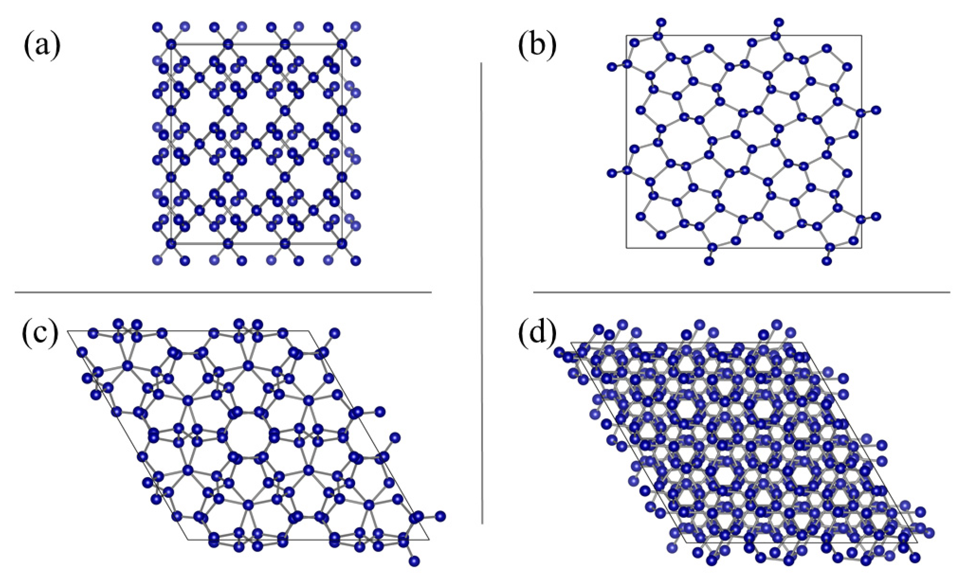
Figure 1. 2 × 2 unit cell structures of (a) 135-3-40-C-r89-np-id355667 with pure sp 2 hybridization, (b) 136-3-20-C-r689-np-id545421_1 with hybrid sp 2 / sp 3 hybridization, (c) 179-3-36-C-r6789-p-id545421 with pure sp 3 hybridization, and (d) 165-3-28-C-r68-np-id545421 with pure sp 3 hybridization.
Crystals 11 00783 g001
Figure 2. Phonon dispersion of (a) 135-3-40-C-r89-np-id355667, (b) 136-3-20-C-r689-np-id545421_1, (c) 179-3-36-C-r6789-p-id545421, (d) 165-3-28-C-r68-np-id545421.
Crystals 11 00783 g002
Figure 3. Pearson correlation matrix between Vickers’ hardness from Tian’s model ( V H T i a n ), universal anisotropy (AU), shear modulus ( G ), Pugh’s ratio ( k ), bulk modulus ( B ), elastic modulus ( E ), Poisson’s ratio ( ν ), density (ρ), volume per atom (VPA), packing fraction (PF), and average local potential (Avg. LOCPOT).
Crystals 11 00783 g003
Figure 4. 2D map of bulk modulus vs. shear modulus, with Pugh’s ratio as color bar to explain hardness and show the relationship between all the mentioned properties.
Crystals 11 00783 g004
Figure 5. 2D map of bulk modulus vs. shear modulus with Poisson’s ratio as color bar to explain hardness and show the relationship between all the mentioned properties.
Crystals 11 00783 g005
Table 1. Some representative carbon allotropes with different hybridizations.
MaterialsHybridizationsVickers’ Hardness, (GPa)Ground-State Energy, (eV)Average Local Potential, (eV)
(a) 135-3-40-C-r89-np-id355667 sp 2 30.88994−341.2203−11.7709
(b) 136-3-20-C-r689-np-id545421_1Hybrid sp 2 /   sp 3 69.35087−175.5362−12.7828
(c) 179-3-36-C-r6789-p-id545421 sp 3 90.11029−320.6033−12.9213
(d) 165-3-28-C-r68-np-id545421 sp 3 90.10081−245.7932−13.1631
Table 2. Carbon allotropes with high Vickers’ hardness with other material properties.
MaterialsVickers’ Hardness, (GPa)Universal AnisotropyBulk Modulus, (GPa)Elastic Modulus, (GPa)Poisson’s Ratio Density ,   ( kg / m 3 ) Volume Per AtomPacking FractionAverage Local Potential, (eV)
206-1-16-C-r0-np-id355667104.3020.00457385.281060.730.041143.55345.612720.25595−13.467
181-1-6-C-r0-p-id224838_194.85070.04505429.821108.010.070363.91255.712630.2515−13.185
154-1-6-C-r0-p-id22483894.361590.044264431.97351109.8130.0718053.4961095.7046950.251855−13.195
180-1-12-C-r0-p-id22483894.167930.055942428.27631102.0330.0711363.4858965.721410.251119−13.169
182-1-12-C-r6x-p-id22483894.134540.084798433.42821111.4860.0725993.4876365.7185540.251244−13.169
Table 3. Carbon allotropes with low Vickers’ hardness with other material properties.
Materials Vickers’ Hardness, (GPa)Universal Anisotropy Bulk Modulus, (GPa)Elastic Modulus, (GPa)Poisson’s Ratio Density ,   ( kg / m 3 ) Volume Per AtomPacking FractionAverage Local Potential (eV)
224-3-72-C-r69-np-id3556672.999861.5687399.0780187.231160.3532621.56168612.770970.112502−8.092
131-2-48-C-r68x-np-id2248383.0823822.944065170.7716125.98870.377042.0743429.614730.149433−9.773
207-3-72-C-r689-np-id2248381.1628791.08592566.6758842.139260.3946661.27629615.626660.091943−6.915
222-3-112-C-r6x-np-id3556671.5411331.974846118.857170.426620.4012451.47788713.49510.106465−7.750
155-3-54-C-r6x-p-id3556673.3189812.3367269.394472.491720.3258941.54156912.937620.111052−8.030
Publisher’s Note: MDPI stays neutral with regard to jurisdictional claims in published maps and institutional affiliations.

