Numerical Model Study of Multiple Dendrite Motion Behavior in Melt Based on LBM-CA Method

Abstract

In this paper, a new method is proposed to solve the solute field of moving grains, and a Cellular automaton (CA)-Lattice Boltzmann method (LBM)-Semi rebound format(Ladd) coupling model which can accurately simulate the motion behavior of multiple dendrites is established. The growth process of microstructure in the solidification process of Al-4.7% Cu alloy ingot was calculated by Cellular automaton (CA) method, the momentum, heat, and mass transfer processes were calculated by Lattice Boltzmann method (LBM), and the melt-dendrite sharp interface interaction was treated by Ladd method. The reliability of the model is verified, and then the growth and movement of single dendrite and multiple dendrites under the action of gravity field are simulated. The simulation results show that the growth and movement mode of multiple dendrites are quite different from that of single dendrite, which is shown in two aspects: (1) the original motion state of dendrites is changed by the combination of flow field, which slows down the falling speed of dendrites to a certain extent; (2) the fusion of solute field between dendrites changed the original growth mode of boundary dendrites and increased their rotation speed.

1. Introduction

During the solidification process of the alloy, the fine grains formed on the surface of the mold will fall off, and the solidified dendrite arms will also be remelted and fractured, resulting in a large number of free equiaxed dendrites in the liquid phase area, which will move under the action of natural convection and gravity [1]. The movement and falling process of a large number of group grains not only has an important influence on the formation of positive segregation at the top of ingot, A-type and V-type segregation [2], but also is the main reason for the formation of triangular cone-shaped negative segregation at the bottom of large ingot [3,4].Therefore, it is of great significance to add the calculation of grain movement process into the numerical model of ingot macrosegregation to improve the prediction accuracy.

At present, the phase field method is mostly used to simulate grain movement in the world. In 2008, Do-Quang M et al. [5] used the phase field-virtual domain method to simulate the growth and movement of single dendrite under the action of gravity. In 2012, karagadde and Bhattacharya [6] used the enthalpy method (EF) to calculate the growth of dendrites, the volume of fluid method (VOF) to calculate the movement behavior of dendrites, and the immersion boundary method (IBM) to deal with the solid-liquid interface. The simulation results show that the multi dendrite growth pattern is significantly different from that of the single dendrite. In 2013, Medvedev et al. [7] used Phase Field-Lattice Boltzmann method (LBM) coupling model to calculate the dendrite growth and movement behavior of aluminum copper alloy under the action of shear flow and pipe flow. In 2015, Rojas and Takaki [8] used a PF-LBM model to simulate the growth and movement of dendrites under shear flow, and analyzed the effect of solution flow on the growth and movement of dendrites. In the same year, Takaki et al. [9] added GPU technology to the program code, which greatly improved the simulation efficiency and scale, and used the technology to simulate the settlement behavior of single dendrite in the gravity field. In 2017, Qi et al. [10] proposed a new phase-field model incorporating dendrite-melt two-phase flow, and modified the boundary layer of growth kinetics equation, so that it can better reflect the relationship between the growth rate of dendrite tip and the flow direction of fluid. In 2018, Takaki et al. [11] established a new phase field model to simulate the growth and movement of multi-dendrite, and coupled this model with lattice Boltzmann to simulate the growth, movement, collision, and growth behavior after bonding of multi-dendrite.

However, the grid of phase field method is very small and the amount of calculation is huge, which greatly limits the number of equiaxed dendrites. It is impossible to simulate the solidification process of ingots with a large number of equiaxed and columnar dendrites [12]. The Cellular automaton (CA) method has a small amount of calculation and a fast calculation speed, and is undoubtedly more suitable for calculating multi-dendritic motion behavior. Currently, only the work of Liu et al. [13] used the CA method to calculate the moving dendrite. He can only simulate the settlement of a single dendrite, and the dendrite cannot rotate, obviously this is different from the actual situation. This paper improves the calculation accuracy of the concentration field and simulates the movement of multiple dendrites.

In addition, the temperature, flow, and solute fields need to be calculated when simulating dendrite motion in the melt. The LBM method developed in recent years can effectively calculate the passage process of dendrites in the melt, so it has been widely used. This paper uses the LBM method to calculate three fields. The dendrite in the melt must interact with the melt during the movement. This article uses the Ladd method to deal with this effect, because the Ladd method uniformly processes the solid phase and the liquid phase, so as to avoid the mass and momentum loss caused by the solid phase node covering the liquid phase node in the process of dendrite movement. However, the difficulty in dealing with the solid-liquid interaction lies in the calculation of the solute field. The solute diffusion coefficient of the two phases is quite different, therefore it cannot directly treat the two phases as a whole to deal with the boundary. Therefore, this paper presents a method to deal with the solute field of multi grain movement, which realizes the calculation of solute field in the real sense of dendrite movement.

2. Materials and Methods

In this paper, Al-4.7% Cu alloy is selected as the research object, and the physical parameters are shown in

Table 1. Physical properties of Al-4.7% Cu alloy.

Physical Parameter	Symbol	Value
Melting temperature	Tm (K)	933.3
Liquidus temperature	TL (K)	917
Solidus temperature	TS (K)	821
Liquidus slope	M (m·K/%)	−3.44
Thermal diffusivity	A (m2·s−1)	2.7 × 10−7
Fluid viscosity	Ν (m2·s−1)	1.2 × 10−6
Diffusivity in liquid	D (m2·s−1)	3.0 × 10−9
Partition coefficient	k	0.145
Liquid density	Ρ (kg·m−3)	2606

.

2.1. CA Model

The solute equilibrium model (ZS model) proposed by Zhu [14] is used in this paper. The growth driving force is the difference between the equilibrium crystallization concentration and the actual liquid concentration at the interface. The actual liquid concentration $C_L$ can be calculated by LBM, and the equilibrium crystallization concentration $C_L^{eq}$ can be calculated by the following formula according to the equilibrium crystallization theory:

$$C_L^{eq}=C_0+[T_L^{}-T_L^{eq}+\Gamma Kf(\varphi ,{\theta }_0)]/m$$

(1)

where $C_0$ is the initial concentration of the alloy; m is the slope of the liquidus; T_L is the actual temperature of the interface; $T_L^{eq}$ is the liquidus temperature at the initial concentration of $C_0$, $\Gamma$ is the Gibbs Thomson coefficient; K is the average curvature at the solid/liquid interface, $f(\varphi ,{\theta }_0)$ is the anisotropic function of the interface energy. K can be calculated from the spatial distribution of the interface solid phase ratio.

$$K={[{(\frac{\partial f_S}{\partial x})}^2+{(\frac{\partial f_S}{\partial y})}^2]}^{-3/2}\cdot [2\frac{\partial f_S}{\partial x}\frac{\partial f_S}{\partial y}\frac{{\partial }^2{f}_S}{\partial x\partial y}-{(\frac{\partial f_S}{\partial x})}^2\frac{{\partial }^2{f}_S}{\partial y^2}-{(\frac{\partial f_S}{\partial y})}^2\frac{{\partial }^2{f}_S}{\partial x^2}]$$

(2)

According to the Gibbs-Thomson formula, the interface energy anisotropy function in Equation (1) can be expressed as:

$$f(\varphi ,{\theta }_0)=\Psi (\varphi ,{\theta }_0)+\frac{{\partial }^2}{\partial {\varphi }^2}\Psi (\varphi ,{\theta }_0)=1-\delta \cos [4(\varphi -{\theta }_0)]$$

(3)

where $\delta =15\epsilon$ is the anisotropy coefficient ($\epsilon$ is the anisotropic strength of the interface energy), $\psi (\varphi ,{\theta }_0)$ is the anisotropy function of the interface energy, $\varphi$ is the angle between the normal direction of the solid-liquid interface and the horizontal direction, and ${\theta }_0$ is the preferred growth direction. The anisotropy function $\psi (\varphi ,{\theta }_0)$ and the growth angle $\varphi$ can be calculated from Equations (4) and (5).

$$\psi (\varphi ,{\theta }_0)=1+\epsilon \cos [4(\varphi -{\theta }_0)]$$

(4)

$$\varphi =\{\begin{array}{ll}{\cos }^{-1}[\frac{\partial f_S}{\partial x}{[{(\frac{\partial f_S}{\partial x})}^2+{(\frac{\partial f_S}{\partial y})}^2]}^{-1/2}]& \frac{\partial f_S}{\partial y}\ge \mathbf{0}\\ \mathbf{2}\pi -{\cos }^{-1}[\frac{\partial f_S}{\partial x}{[{(\frac{\partial f_S}{\partial x})}^2+{(\frac{\partial f_S}{\partial y})}^2]}^{-1/2}]& \frac{\partial f_S}{\partial y}<\mathbf{0}\end{array}$$

(5)

When $C_L<C_L^{eq}$, the solid fraction increment $\Delta f_s$ in a time step is calculated by the following formula:

$$\Delta f_S=\frac{(C_L^{eq}-C_L^{})}{C_L^{eq}(1-k)}$$

(6)

In order to partially eliminate anisotropy, this paper uses an improved eight-neighbor capture method proposed by Zhu [15].

2.2. LBM Model

According to Boussinesq’s approximation, the effect of latent heat and solutes on the density during the solidification process can be expressed by the following formula:

$$\rho ={\rho }_0[1-{\beta }_T(T-T_0)-{\beta }_C(C-C_0)]$$

(7)

where ${\rho }_0$, $T_0$, and $C_0$ represent the initial density, temperature, and concentration of the liquid phase, respectively, and $T$ and $C$ are the temperature and concentration of the liquid phase at the current moment. ${\beta }_T$ and ${\beta }_C$ are the volume expansion coefficients of temperature and concentration changes, respectively. The resultant force of the fluid particles is:

$$\begin{array}{ll}\mathit{F}& =\mathit{g}{\rho }_0[1-{\beta }_T(T-T_0)-{\beta }_C(C-C_0)]+(-{\rho }_0\mathit{g})\\ & =\mathit{g}{\rho }_0[-{\beta }_T(T-T_0)-{\beta }_C(C-C_0)]\end{array}$$

(8)

The distribution function of the flow field can be expressed as:

$$f_i(\mathit{x}+{\mathit{e}}_i\Delta t,t+\Delta t)=f_i(\mathit{x},t)+\frac{1}{{\tau }_f}(f_i^{eq}(\mathit{x},t)-f_i(\mathit{x},t))+F_i$$

(9)

where $F_i$ is the component force of the particle under the external force field in the i direction, and its magnitude is expressed as:

$$F_i=(1-\frac{1}{2{\tau }_f}){\omega }_i[3\frac{{\mathit{e}}_i-\mathit{u}}{c^2}+9\frac{{\mathit{e}}_i\cdot \mathit{u}}{c^4}]\Delta t\cdot \mathit{F}$$

(10)

where ${\omega }_i$ is the weight coefficient in each direction, which represents the probability of particles moving in different directions, which can be expressed as:

$${\omega }_i=\{\begin{array}{ll}4/9& i=0\\ 1/9& i=1,2,3,4\\ 1/36& i=5,6,7,8\end{array}$$

(11)

The equilibrium distribution function and relaxation time of the flow field in Equation (9) are respectively expressed as:

$$f_i^{eq}(\mathit{x},t)={\omega }_i\rho (1+3\frac{{\mathit{e}}_i\cdot \mathit{u}}{c^2}+\frac{9}{2}\frac{{({\mathit{e}}_i\cdot \mathit{u})}^2}{c^4}-\frac{3}{2}\frac{\mathit{u}\cdot \mathit{u}}{c^2})$$

(12)

$${\tau }_f=3\nu /(c^2\Delta t)+0.5$$

(13)

where $\nu$ is the dynamic viscosity of the fluid. The macroscopic density $\rho$ and velocity $u$ are obtained by adding the distribution function.

$$\rho ={\displaystyle \sum _{i=0}^8{f}_i}$$

(14)

$$\mathit{u}=({\displaystyle \sum _{i=0}^8{\mathit{e}}_i}{f}_i+\mathit{F}\cdot \Delta t/2)/\rho$$

(15)

The distribution functions of temperature field and solute field are similar to those of flow field:

$$h_i(\mathit{x}+{\mathit{e}}_i\Delta t,t+\Delta t)=h_i(\mathit{x},t)+\frac{1}{{\tau }_{\alpha }}(h_i^{eq}(\mathit{x},t)-h_i(\mathit{x},t))+H_i$$

(16)

$$g_i(\mathit{x}+{\mathit{e}}_i\Delta t,t+{\Delta }_{}t)=g_i(\mathit{x},t)+\frac{1}{{\tau }_D}(g_i^{eq}(\mathit{x},t)-g_i(\mathit{x},t))+G_i$$

(17)

where $h_i(x,t)$ and $g_i(x,t)$ are the distribution functions of temperature field and solute field at the position x at time t, respectively, and $h_i(x,t)$ and $g_i(x,t)$ represent the temperature field and the equilibrium distribution function of the solute field, respectively defined as:

$$h_i^{eq}(\mathit{x},t)={\omega }_{i}T(1+3\frac{{\mathit{e}}_i\cdot \mathit{u}}{c^2}+\frac{9}{2}\frac{{({\mathit{e}}_i\cdot \mathit{u})}^2}{c^4}-\frac{3}{2}\frac{\mathit{u}\cdot \mathit{u}}{c^2})$$

(18)

$$g_i^{eq}(\mathit{x},t)={\omega }_{i}C(1+3\frac{{\mathit{e}}_i\cdot \mathit{u}}{c^2}+\frac{9}{2}\frac{{({\mathit{e}}_i\cdot \mathit{u})}^2}{c^4}-\frac{3}{2}\frac{\mathit{u}\cdot \mathit{u}}{c^2})$$

(19)

The relaxation time ${\tau }_{\alpha }$ in the temperature field and the relaxation time ${\tau }_D$ in the solute field can be obtained by using the corresponding diffusion coefficients:

$${\tau }_{\alpha }=3\alpha /(c^2\Delta t)+0.5$$

(20)

$${\tau }_D=3D/(c^2\Delta t)+0.5$$

(21)

where $\alpha$ is a temperature diffusion coefficient, and $D$ is a concentration diffusion coefficient. Macro temperature and concentration are:

$$T={\displaystyle \sum _{i=0}^8{h}_i}(\mathit{x},t);C={\displaystyle \sum _{i=0}^8{g}_i(\mathit{r},t)}$$

(22)

The source term $H_i$ of the temperature field and the source term $G_i$ of the concentration field can be expressed as:

$$H_{\mathrm{i}}={\omega }_i\Delta T;G_{\mathrm{i}}={\omega }_i\Delta C$$

(23)

In the formula, $\Delta T$ and $\Delta H$ respectively represent the latent heat released by the solidification of the alloy and the excluded solutes.

2.3. Ladd Method to Calculate the Solid-liquid Interface Interaction Force

In Figure 1, $x_b$ is the particle boundary point, $x_l$ is the liquid phase lattice point of the boundary node along the $c_{-i}$ direction, $x_s$ is the solid phase lattice point of the boundary node along the $c_i$ direction, and $u_b$ is the particle velocity. The calculation formulas of $x_s$ and $x_b$ are:

$$x_s=x_l+\Delta t\cdot c_i$$

(24)

$$u_b=V_b+W_b\left(x_b-x_c\right)$$

(25)

where $\Delta t$ is the time step, $V_b$ and $W_b$ are the translational and rotational speeds, respectively, and $x_c$ is the center of mass of the solid particles. The solid-liquid distribution functions at time t are $f_i(x_l,t)$ and $f_{-i}(x_s,t)$. After $\Delta t/2$ time, the two particles move to the boundary and collide. The distribution function at this time is:

$$f_{-i}^{}(x_b,t+\Delta t/\mathbf{2})=f_i^{}(x_l,t)+\mathbf{2}{\omega }_{-i}\rho \frac{c_{-i}{u}_b}{c_s^2}$$

(26)

$$f_i^{}(x_b,t+\Delta t/\mathbf{2})=f_{-i}^{}(x_s,t)+\mathbf{2}{\omega }_i\rho \frac{c_i{u}_b}{c_s^2}$$

(27)

After the $\Delta t/2$ time, the fluid particles bounce to the corresponding lattice points respectively. At this time, the distribution functions of the liquid phase and solid phase lattice points are:

$$f_{-i}^{}(x_l,t+\Delta t)=f_{-i}^{}(x_b,t+\Delta t/\mathbf{2})$$

(28)

$$f_i^{}(x_s,t+\Delta t)=f_i^{}(x_b,t+\Delta t/\mathbf{2})$$

(29)

Force exerted by fluid particles on solid particles:

$$F_i=\frac{\Delta x^2}{\Delta t}\left[f_{-i}\left(x_f,t+\Delta t\right)+f_i\left(x_f,t\right)-f_i\left(x_s,t+\Delta t\right)-f_{-i}\left(x_s,t\right)\right]c_i$$

(30)

The total force $F$ on the solid particles is:

$$F=\frac{\Delta x^2}{\Delta t}{\displaystyle \sum _{{\mathrm{x}}_b}{\displaystyle \sum _i[f_{-i}(x_f,t+\Delta t)+f_i^{}(x_f,t)-f_i^{}(x_s,t+\Delta t)-f_{-i}(x_s,t)]}}{c}_i$$

(31)

The force moment on the solid particles is:

$$T_{\mathrm{t}}={\displaystyle \sum _{x_b}{F}_{x_b}}\left(x_b-x_c\right)$$

(32)

According to Newton’s second law, the translation speed and rotation speed of the grains can be calculated respectively as:

$$V=\frac{F+G}{M_S}dtW=\frac{T_{\mathrm{t}}}{I_S}dt$$

(33)

where $M_S$ and $I_S$ are mass and moment of inertia, respectively, and $G$ is the combined force of gravity and buoyancy.

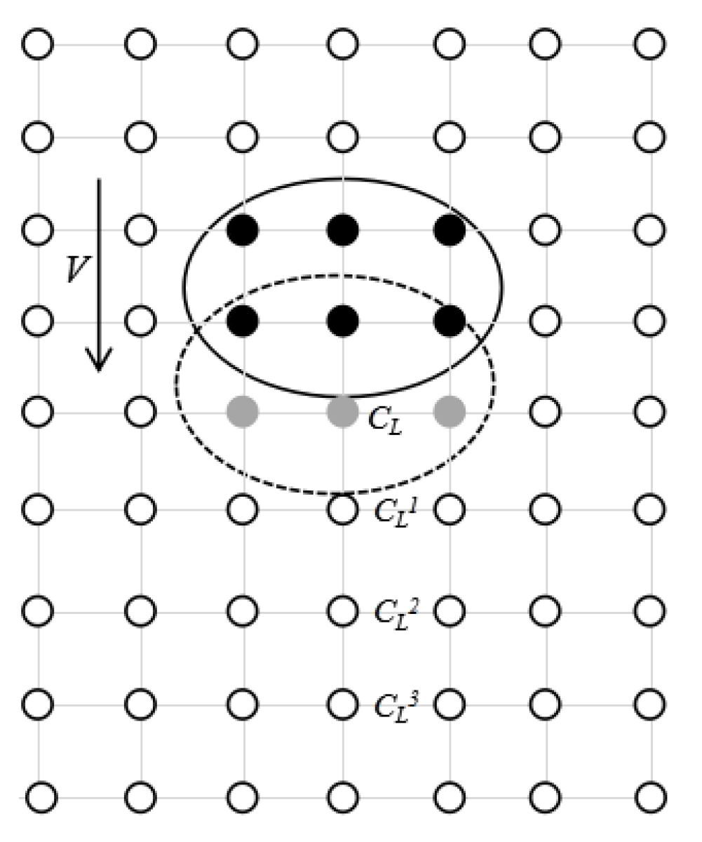
2.4. Processing of Solute Fields at Moving Boundaries

In order to accurately calculate the solute field during movement, a solute extrapolation method for calculating the solute field at the moving boundary is proposed.

As shown in Figure 2, the white and black grid points are the liquid and solid grid points, the solid ellipse is the position of the dendrite at the previous moment, the dotted ellipse is the current position. The gray grid points are the covered liquid nodes because of dendrite movement. The concentration $C_L$ of the covered liquid grid points will be distributed in a certain proportion, which is:

$$\Delta C_L^1=A\cdot C_L\Delta C_L^2=B\cdot C_L\Delta C_L^3=C\cdot C_L$$

(34)

$\Delta C_L^1$,$\Delta C_L^2$, and $\Delta C_L^3$ respectively represent the concentration assigned to three lattice points along the direction of dendrite movement. The distance between the lattice points is the grain movement distance. $A$, $B$, and $C$ are the distribution coefficients and satisfy the following relations:

$$A+B+C=1A>B>C$$

(35)

In this paper, the undetermined coefficient method is used, and the distribution coefficients of different proportions are used to calculate. Then the results are compared with the experimental results of Liu’s single dendrite drop. The empirical values of $A$, $B$, and $C$ are 0.7, 0.2, and 0.1, respectively. The assigned concentration will be added to the three lattice points along the direction of dendrite movement.

$$C_L^n=C_L^n+\Delta C_L^n$$

(36)

3. Verification

First, the accuracy of the Ladd method for processing moving boundaries is evaluated through the settlement process of circular particles in an infinitely long pipe. Then, the accuracy of the solute distribution model established in this paper is verified by calculating the solute field conservation of the single dendrite in the moving state. The LBM model, the dendrite growth of CA model, and the rationality of the single dendrite movement model have been confirmed in relevant researches [16,17], so this article will not be described here.

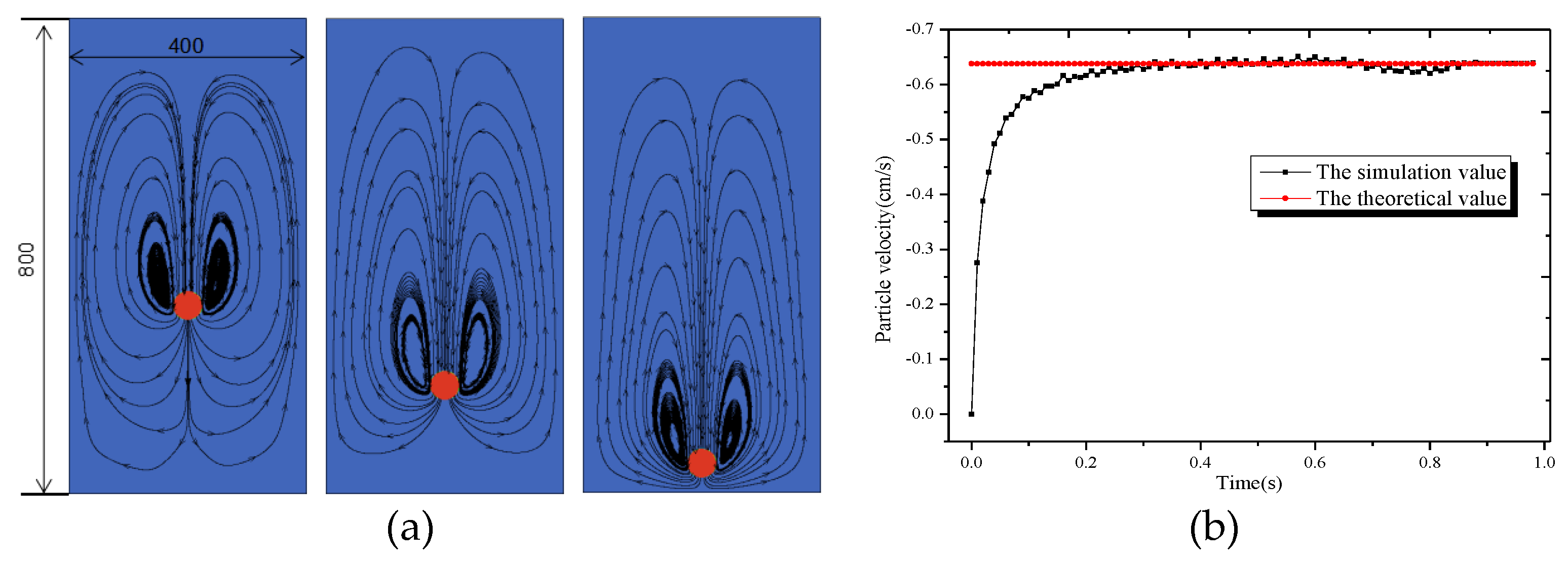
3.1. Settling of a Circular Particle in an Infinitely Long Tube

The circular particle accelerates to settle down in the infinite tube due to gravity. As the speed increases, the resistance of the ball increases. When the three forces of resistance, gravity, and buoyancy are balanced, the particle falls at a uniform speed. Glowinski pointed out in the literature [18] that, for a circular particle settling in an infinitely long pipe, when its physical parameters are determined, the settling speed is also determined at a steady state.

When the liquid is at a low Reynolds number, the resistance Ff to circular particles moving in an infinitely long pipeline is directly proportional to the settlement speed [19] and can be expressed as:

$$F_f=4\pi K\eta v$$

(37)

where $v$ is the falling velocity of circular particles, $\eta$ is the dynamic viscosity of the fluid, $K$ is the correction factor, and its value reflects the influence of the resistance of the pipe wall facing the particles. $K$ is expressed as:

$$K=\frac{1}{\ln W_{\mathrm{i}}-0.9157+1.7244{(W_i)}^{-2}-1.7302{(W_i)}^{-4}+2.4056{(W_i)}^{-6}-4.5913{(W_i)}^{-8}}$$

(38)

where $W_i=W/D$, $W$ is the width of a long square tube and $D$ is the diameter of the circular particle. When particles are in a state of three forces equilibrium, the resistance can be obtained as:

$$F_f=\frac{1}{4}\pi D^2({\rho }_S-{\rho }_{\mathrm{L}})g$$

(39)

${\rho }_S$ and ${\rho }_L$ are solid density and liquid density, and g is gravity acceleration. According to Equations (37)–(39), the final falling speed of the circular particle can be calculated as:

$$v=\frac{D^2({\rho }_S-{\rho }_f)\mathbf{g}}{16K\eta }$$

(40)

The size of the circular pipe in this paper is 4 cm × 8 cm. The side length of each grid is 0.01 cm, with a total of 400 × 800 grids. The particle diameter is taken as 0.48 cm, the fluid density is ${\rho }_L=1.0 \mathrm{g}/\mathrm{c}{\mathrm{m}}^3$ and the solid density is ${\rho }_S=1.02 \mathrm{g}/\mathrm{c}{\mathrm{m}}^3$, and the fluid viscosity is $\eta =0.33 \mathrm{g}/(\mathrm{c}\mathrm{m}·\mathrm{s})$. The relaxation time $\tau$ is taken as 0.8, and the gravity acceleration is $g=980.0 \mathrm{c}\mathrm{m}/{\mathrm{s}}^2$. At the initial moment, the circular particle are placed at points (2 cm, 6 cm), and they are at rest before the calculation starts.

The simulation results are shown in Figure 3. The particle dropped due to gravity, and two symmetrical vortices formed on both sides of the particle, which is consistent with what Do-Quang [5] described in his literature. According to the simulation value of particle settlement speed, it can be seen that the simulation results in this paper agree well with the theoretical analytical solution. Therefore, the method used in this paper can be used to calculate the moving boundary problem.

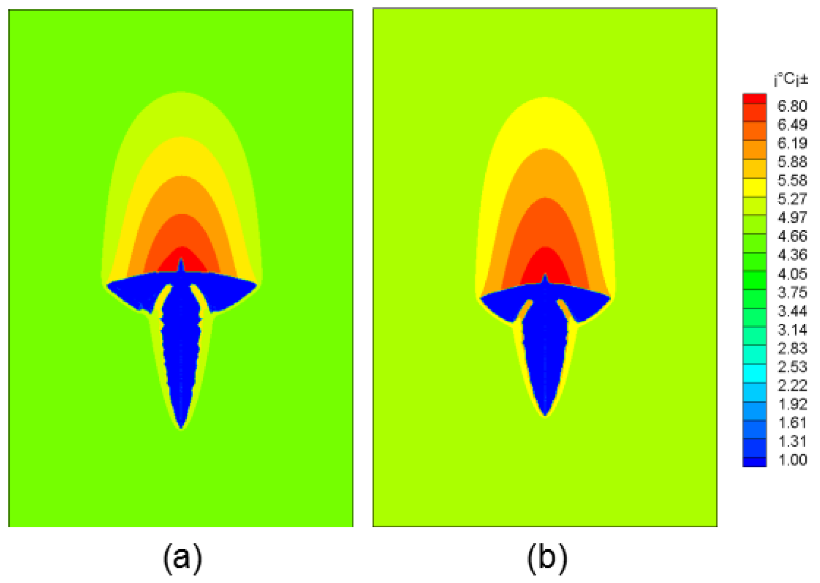
3.2. Calculation of the Solute Field

Figure 4 shows the morphology of dendrite growth under different solute field treatment methods. Figure 4a is the solute distribution method and Figure 4b is the solute extrapolation method.

In the first method, the lower end of the dendrite grew faster, because the dendrite covered the original high-concentration solute domain during the settlement of the dendrite. Through the uniform distribution of solutes, the solute gradient at the upstream end of the dendrite is reduced, so it has a faster growth rate. In contrast, dendrite growth using the solute extrapolation method was more uniform. This article compares the two methods to calculate the average regional concentration at the time of solidification time of 0.3 s, 0.5 s, 0.7 s. It is found that the solute field of Method 1 changes greatly, and the average solute concentrations at the corresponding moments are 4.682%, 4.673%, 4.658% (standard is 4.7%), solute field conservation is always 4.7% in Method 2. It can be seen that the solute field treatment in the second method is more accurate.

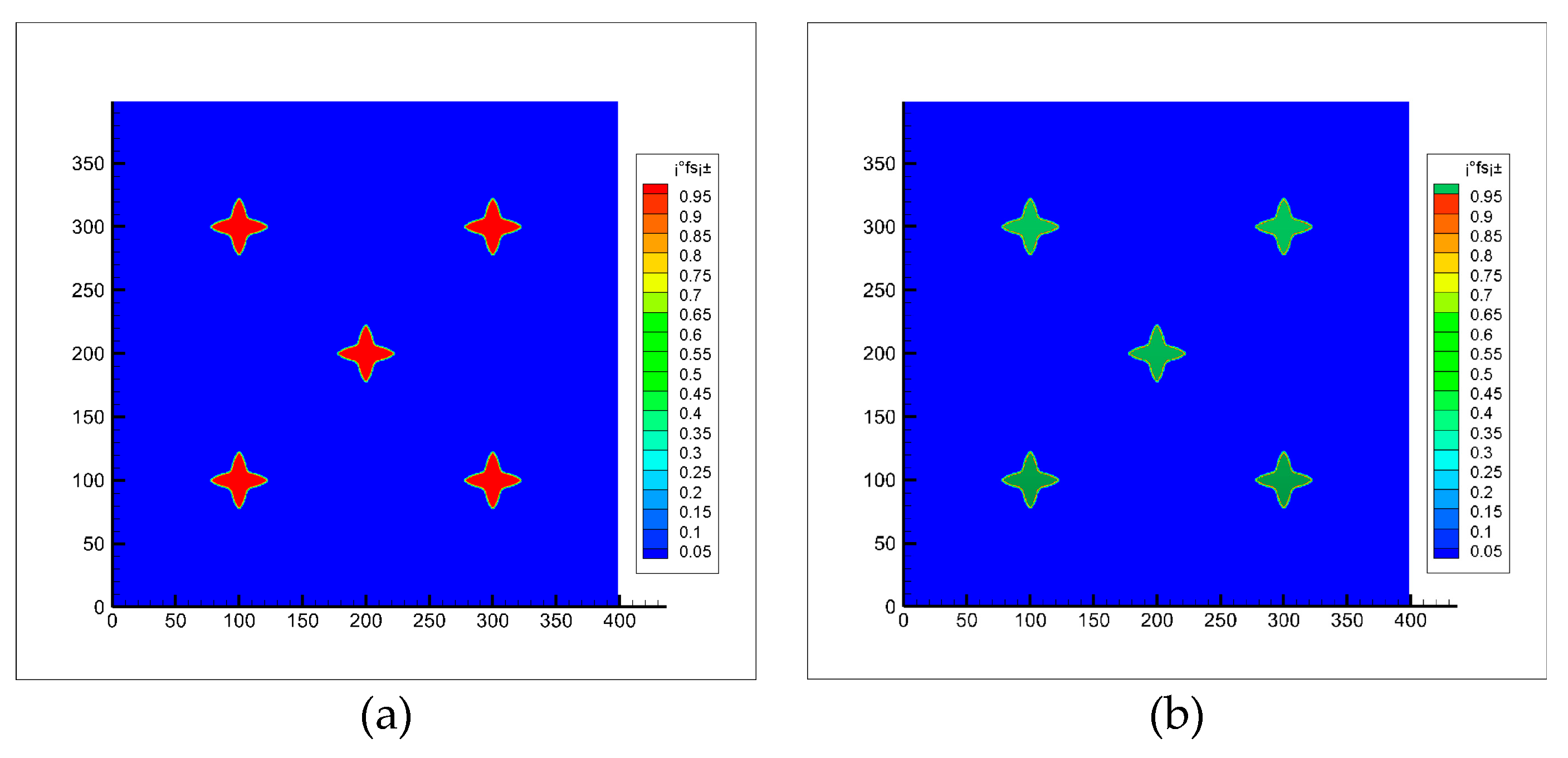
3.3. Multiple Dendrites Rotation

At the initial time, 5 crystal nuclei with preferential growth angles of 0 and a solid phase rate of 0.2 were placed in the middle of the simulation region. When the number of solidification grids is 3000, the dendrites stop growing. At this time, a uniform rotating flow is applied in the simulation region. It can be seen from the Figure 5 that the dendrite can maintain its original shape even after being rotated for multiple turns.

This article gives the formula for calculating the solid phase rate error, as follows:

$$\Delta =(f_{Sin}-f_{S0})/f_{S0}\times 100$$

(41)

where $f_{S0}$ is the initial solid phase rate of the dendrite,$f_{Sin}$ is the solid phase rate after dendrite rotation. According to Equation (41), it is calculated that the change of the solid phase rate of the equiaxed crystal is maintained within 0.2% after 10 revolutions. In the calculations of this paper, the amplitude of dendrite rotation is small (rad <1, rad represents the radian of dendrite rotation), so it can be considered that the numerical model for calculating dendrite rotation established in this paper has no great influence on the dendrite morphology.

4. Discussion

This article is based on the following assumptions. The melt is an incompressible Newtonian fluid. The solid and liquid phases have the same thermal conductivity, and the heat transfer boundary conditions are adiabatic boundary conditions. Solute diffusion only occurs in the liquid phase, there is no solute diffusion in the solid phase, and the boundary condition for mass transfer is the non-diffusion boundary condition [13].

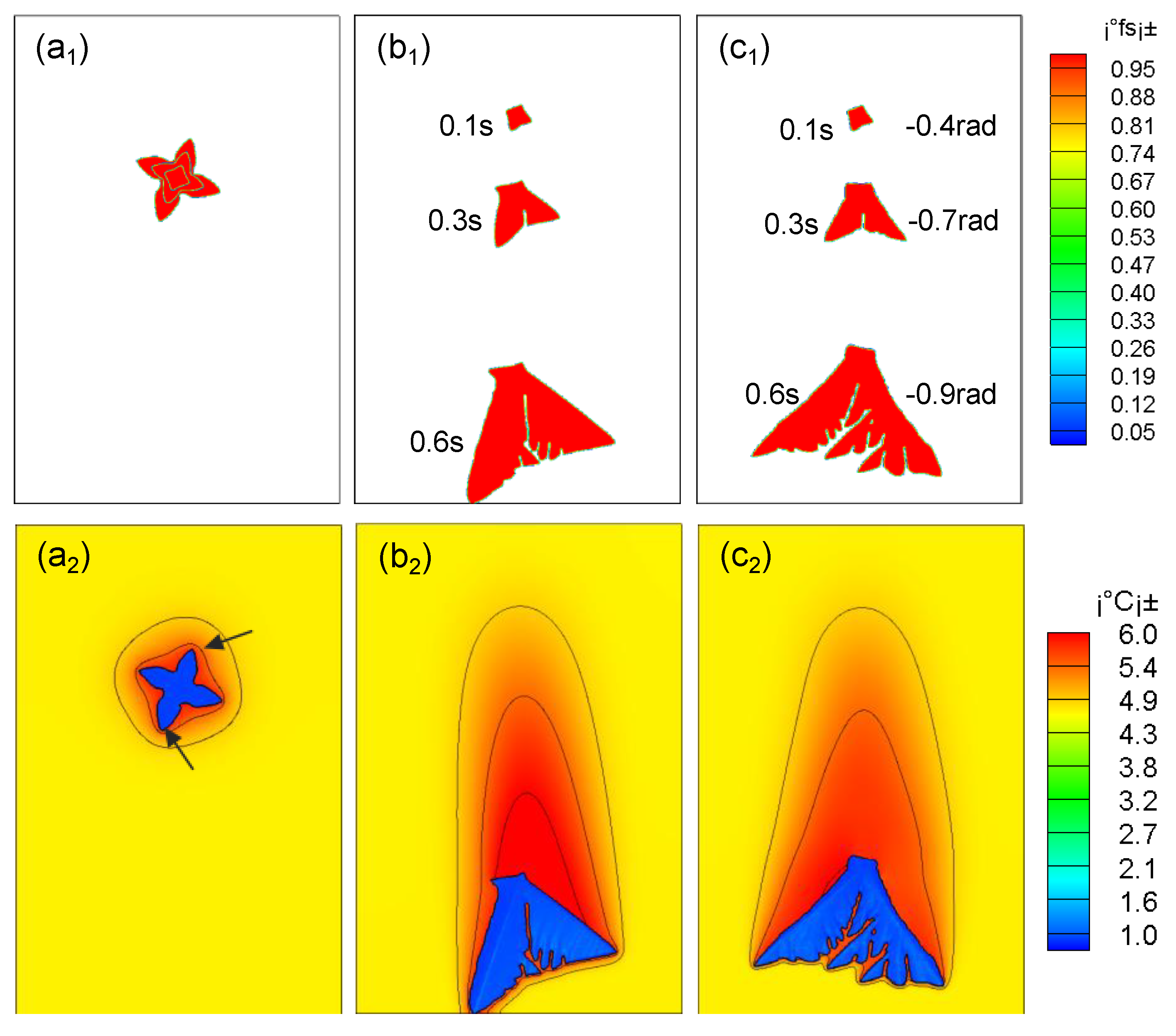
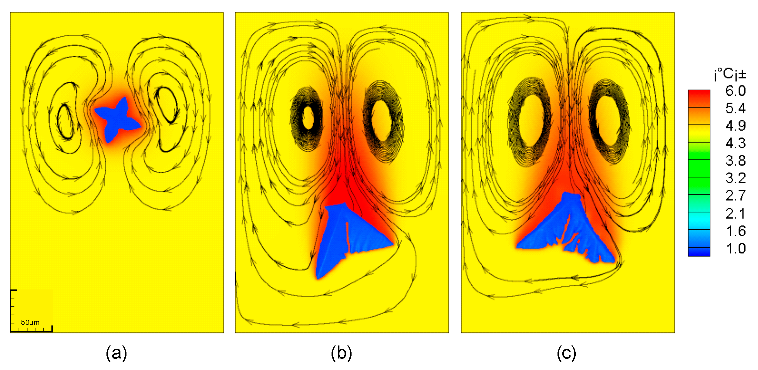
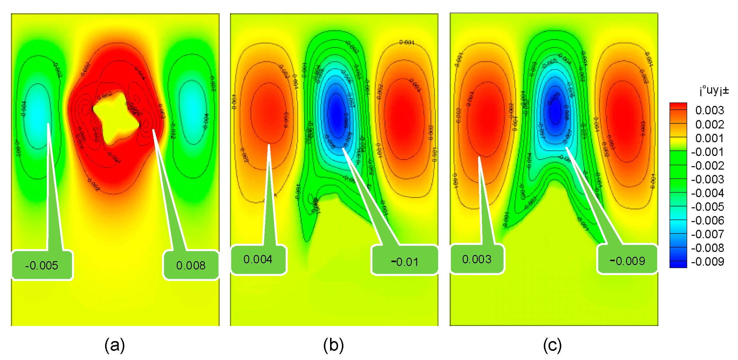
4.1. Single Dendrite Movement

As shown in Figure 6, the dendrite arm at the front end of the dendrite grows faster in the moving state, and a secondary dendrite arm is generated. The upper dendrite arm has a lower speed and almost stops growing. The reason is that the dendrite movement compresses the lower solute boundary layer, the concentration gradient becomes larger, and the temperature gradient becomes lower; the upper solute boundary layer is stretched, the concentration gradient becomes smaller, and the temperature gradient increases. Therefore, the growth of the dendrite arms at the upstream side will be further promoted. As the falling speed increases, this asymmetric growth phenomenon becomes more and more obvious. In actual solidification, when the dendrite grows asymmetrically, the dendrite will rotate. From Figure 6c₂, it can be seen that compared with pure falling dendrites (Figure 6b₂), the former dendrite arms have prominent tips, asymmetric growth is more obvious, and the latter dendrites are more uniform, which is consistent with the literature [6].

The solute distribution is also closely related to the flow of the solution around the dendrites. It can be seen from Figure 7 that the flow direction of the solution is different in the three movement states. The solution near the stationary dendrite flows upward, and the solution far away from the dendrite flows downward. For a moving dendrite, due to the high viscosity of the solution, a downward pulling force will be generated on the surrounding solution during the drop of the dendrite. This causes the solution near the dendrite to flow downwards and the solution away from the dendrites to flow upwards. In addition, for moving dendrites, two vortices will be generated behind it.

It can be seen from Figure 8 that the solution flows faster around the moving dendrites. When the solidification time is 0.5 s, the flow velocity of the solution around the dendrite in the stationary, pure falling, and rotating falling states is 0.008 mm/s, −0.01 mm/s, −0.009 mm/s. This is because the rotation of the dendrite makes the contact surface larger between the lower end and the solution, resulting in an increase in the resistance of dendrites, which reduces the falling speed of the rotating dendrite to a certain extent.

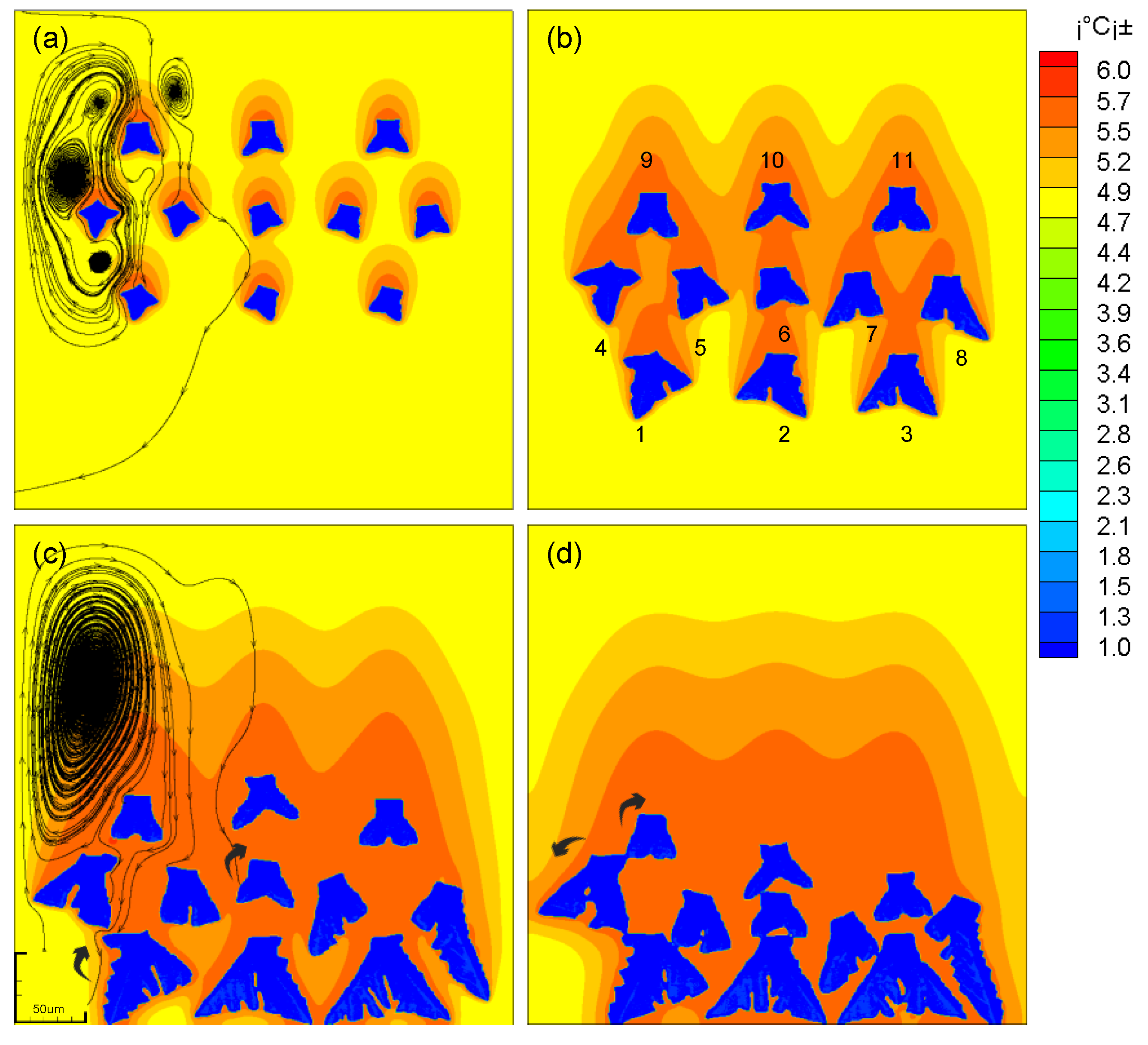
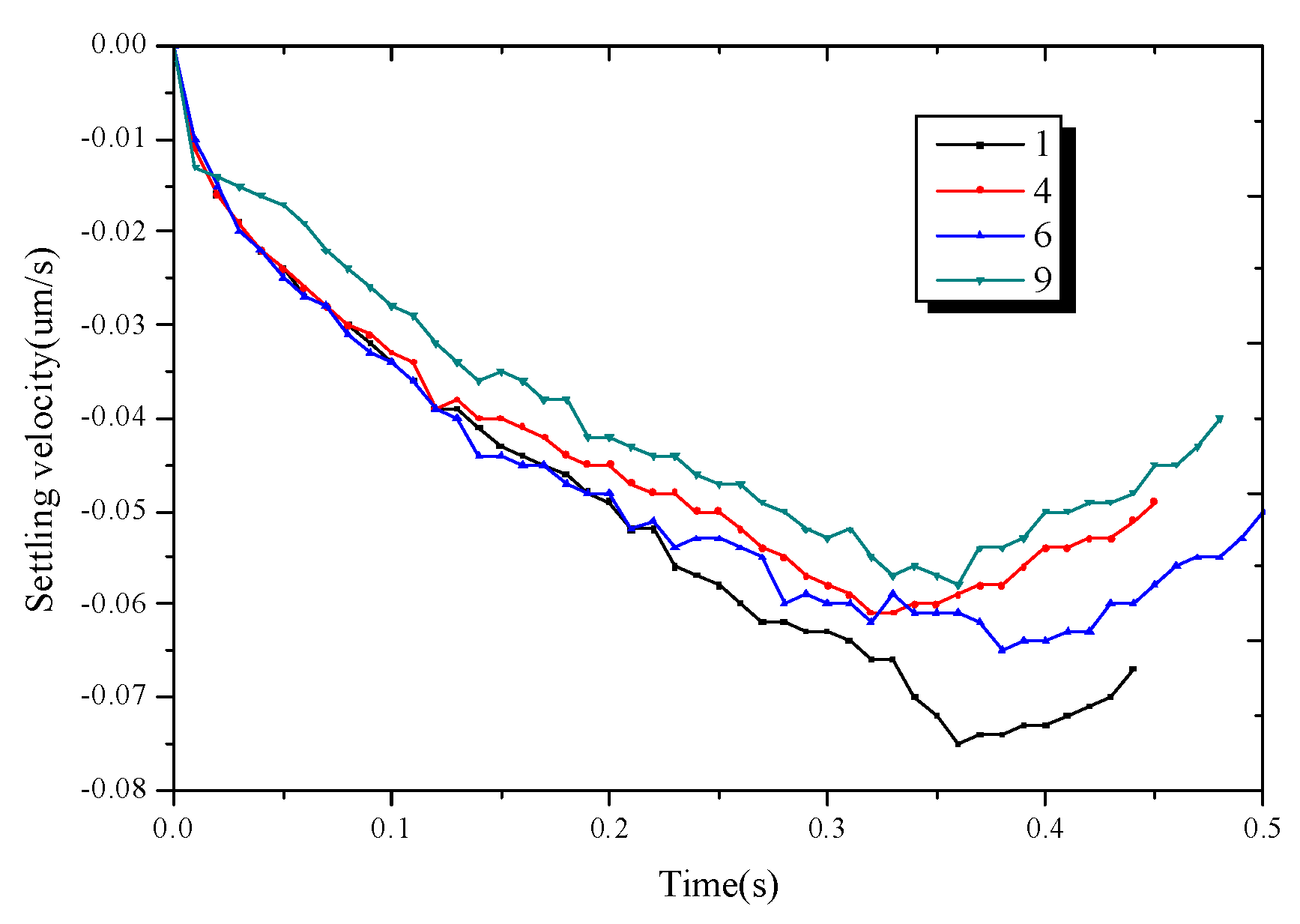
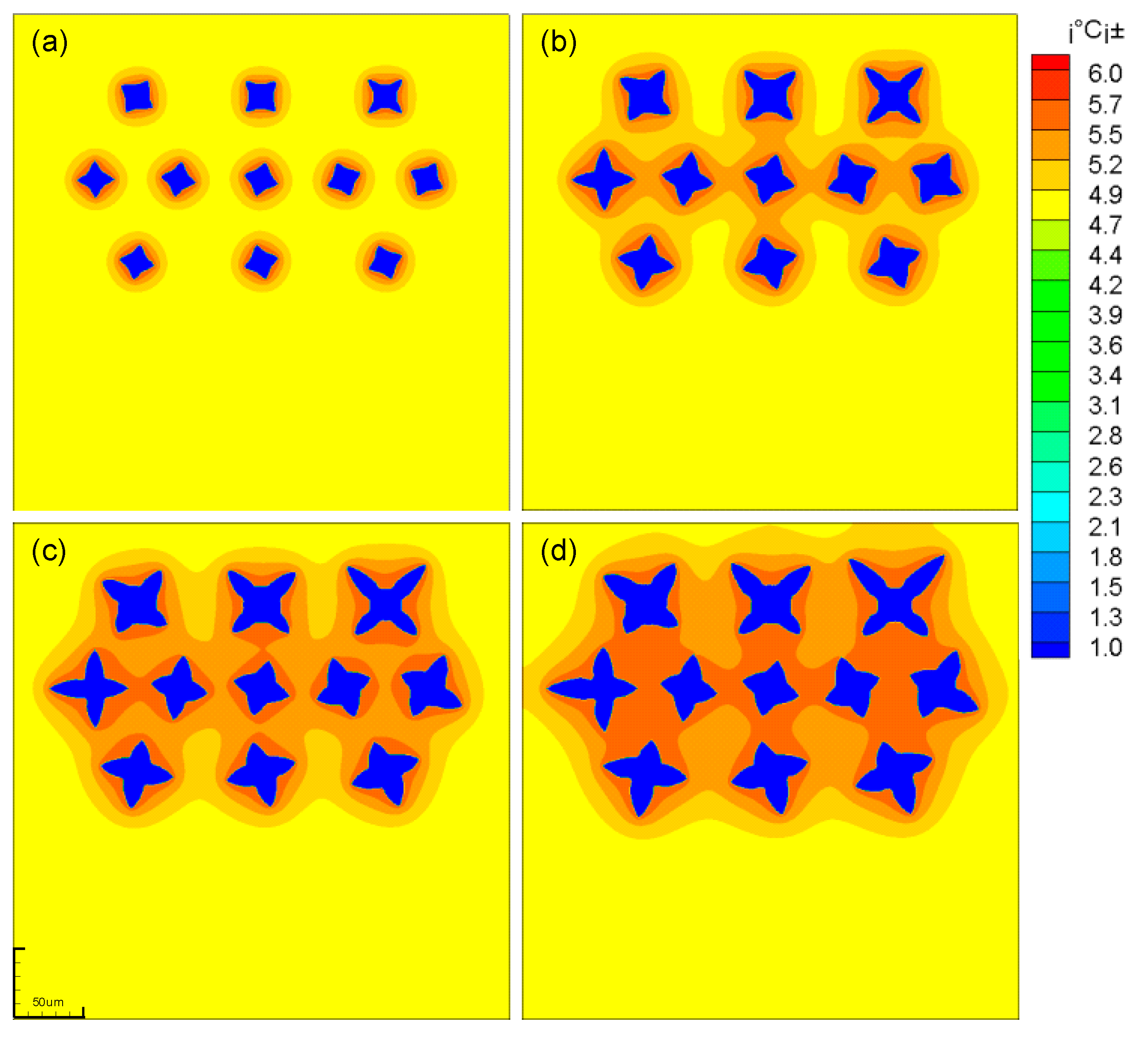
4.2. Multi-Dendrite Movement

As the dendrites grow, the solute boundary layers around the dendrites come into contact and fuse with each other to form a high-concentration solute domain. The growth of dendrite arms in this domain is inhibited, and the growth of dendrite arms away from this domain is promoted. The asymmetry of the dendrite is aggravated, and the rotation speed of the dendrite is increased.

The rotation of dendrites is different from that of single dendrites during solidification. See

Table 2. Preferred growth angle of dendrites at different times.

Dendrite Rotation Angle (rad)
Time (s)	No. 1	No. 4	No. 4	No. 9
0	−0.2	0.1	−0.3	−0.6
0.1	−0.2	0.1	−0.3	−0.6
0.2	−0.3	0	−0.4	−0.7
0.3	−0.4	0	−0.6	−0.8
0.4	−0.5	0.3	−0.6	−0.8
0.5	−0.5	0.5	−0.5	−0.8

for the change of preferential dendrite growth angle. The initial preferred growth angle of No. 4 dendrite is 0.1 rad. The solutes between the dendrites are close to each other and form a high concentration solute domain, therefore the growth of the right dendrite arm of No. 4 dendrite is inhibited, and the growth of the left dendrite arm is promoted. This causes the mass on the left side of the dendrite to be greater than the mass on the right side, so the dendrite is subjected to a counterclockwise torque. When the solidification time is 0.4 s, the dendrite rotates 0.3 rad in a counterclockwise direction. For the No. 1 dendrite, the lower part of the simulated domain is less affected by the solute field. It starts to rotate at 0.2 s and falls to the bottom at 0.5 s. At this time, the preferred growth direction of the dendrite is −0.5 rad. For the No. 9 dendrite, the dendrite arm at the lower end of the dendrite extends to the high-concentration domain, and the growth is inhibited. Therefore, the dendrite is more symmetrical on the left and right, and the torque is less. During its movement, the dendrite only rotated 0.2 rad. The No. 6 dendrite is located in the center of the simulation area. The uncertainty of its growth behavior leads to the complexity of its movement behavior. It can be seen that the dendrite rotates 0.3 rad clockwise when the solidification time is 0.4 s. At 0.5 s, the dendrite rotates counterclockwise by 0.1 rad, and the dendrite rotates left and right.

Multi-dendritic effects are also manifested in interactions between fluids. As shown in Figure 9a, as the dendrites grow, the fluid vortices begin to merge, forming a strong convection between the dendrites. This strong convection hinders the vertical drop of the dendrite and has a lateral force on the dendrite. The dendrite starts to move laterally, and the grains on both sides have a tendency of centrifugal movement. And the movement of the grains in the central domain shows a trend of swinging left and right.

Figure 10 shows the falling speed of the four dendrites. Each dendrite undergoes a process of acceleration and deceleration, and their absolute speeds are lower than those of the single dendrites. It is shown that during the growth of multi-dendritic, due to the interaction between the dendrites, a part of the gravity is offset and the dendrite’s moving speed is reduced to a certain extent.

Compared with the growth of multiple dendrites in the moving state, the growth mode of the dendrites in the stationary state is much simpler. The growth of the dendrites in the middle of the simulated domain is suppressed, and the growth of dendrites near the boundary is promoted. (As shown in Figure 11)

From the above analysis, the movement behavior of multi-dendrites is related to the melt convection and solute overlap between the dendrites. In response to this phenomenon, scholars proposed to apply an external force field (such as an electromagnetic field) to the dendrite to offset gravity, thereby changing the movement state of the dendrite, and then controlling the solute segregation of the casting [20,21].

5. Conclusions

In this work, a CA-LBM-Ladd coupling model for calculating multi-dendritic motion was established, and an extrapolated distribution method for calculating the solute distribution around the dendrite under the state of dendritic motion in the melt was proposed, which realizes the calculation of the solute field in the real state of dendrite movement. The CA-LBM-Ladd coupling model was verified, and then the motion of single and multiple dendrites was simulated using this model. The simulation results show that: 1) the superposition of the flow fields between the multiple dendrites causes the movement state to change; 2) the superposition of solute field results in the change of concentration gradient, changes the growth mode of dendrite, and then changes the movement state. This is quite different from the growth mode of single dendrite.

References

1. Flemings, M.C. Our Understanding of Macrosegregation: Past and Present. Trans. Iron Steel Inst. Jpn. 2000, 40, 838–841. [Google Scholar] [CrossRef]
2. Wu, M.; Ludwig, A.; Bührig-Polaczek, A.; Fehlbier, M.; Sahm, P.R. Influence of convection and grain movement on globular equiaxed solidification. Int. J. Heat Mass Transf. 2003, 46, 2819–2832. [Google Scholar] [CrossRef]
3. Wu, M.; Ludwig, A. Modeling equiaxed solidification with melt convection and grain sedimentation—II. Model verification. Acta Mater. 2009, 57, 5632–5644. [Google Scholar] [CrossRef]
4. Liu, B.; Xu, Q.; Jing, T.; Shen, H.; Han, Z. Advances in multi-scale modeling of solidification and casting processes. JOM 2011, 63, 19–25. [Google Scholar] [CrossRef]
5. Do-Quang, M.; Amberg, G. Simulation of free dendritic crystal growth in a gravity environment. J. Comput. Phys. 2008, 227, 1772–1789. [Google Scholar] [CrossRef]
6. Karagadd, S.; Bhattacharya, A.; Tomar, G.; Dutta, P. A coupled VOF-IBM-enthalpy approach for modeling motion and growth of equiaxed dendrites in a solidifying melt. J. Comput. Phys. 2012, 231, 3987–4000. [Google Scholar] [CrossRef]
7. Medvedev, D.; Varnik, F.; Steinbach, I. Simulating mobile dendrites in a flow. Procedia Comput. Sci. 2013, 18, 2512–2520. [Google Scholar] [CrossRef]
8. Rojas, R.; Takaki, T.; Ohno, M. A phase-field-lattice Boltzmann method for modeling motion and growth of a dendrite for binary alloy solidification in the presence of melt convection. J. Comput. Phys. 2015, 298, 29–40. [Google Scholar] [CrossRef]
9. Takaki, T.; Rojas, R.; Ohno, M.; Shimokawabe, T.; Aoki, T. GPU phase-field lattice Boltzmann simulations of growth and motion of a binary alloy dendrite. IOP Conf. Ser. Mater. Sci. Eng. 2015, 84, 012006. [Google Scholar] [CrossRef] [Green Version]
10. Qi, X.; Chen, Y.; Kang, X.; Li, D.; Gong, T. Modeling of coupled motion and growth interaction of equiaxed dendritic crystals in a binary alloy during solidification. Sci. Rep. 2017, 7, 45770. [Google Scholar] [CrossRef] [Green Version]
11. Takaki, T.; Sato, R.; Rojas, R.; Ohno, M.; Shibuta, Y. Phase-field lattice Boltzmann simulations of multiple dendrite growth with motion, collision, and coalescence and subsequent grain growth. Comput. Mat. Sci. 2018, 147, 124–131. [Google Scholar] [CrossRef]
12. Conti, M. Solidification of binary alloys: Thermal effects studied with the phase-field model. Phys. Rev. E 1997, 55, 765–771. [Google Scholar] [CrossRef]
13. Liu, L.; Pian, S.; Zhang, Z.; Bao, R.; Li, H.; Chen, A. cellular automaton-lattice Boltzmann method for modeling growth and settlement of the dendrites for Al-4.7%Cu solidification. Comput. Mat. Sci. 2018, 146, 9–17. [Google Scholar] [CrossRef]
14. Zhu, M.; Stefanescu, D.M. Virtual front tracking model for the quantitative modeling of dendritic growth in solidification of alloys. Acta Mater. 2007, 55, 1741–1755. [Google Scholar] [CrossRef]
15. Zhu, M.; Hong, C. A modified cellular automaton model for the simulation of dendritic growth in solidification of alloys. ISIJ Int. 2001, 41, 436–445. [Google Scholar] [CrossRef] [Green Version]
16. Yin, H.; Felicelli, S.D.; Wang, L. Simulation of a dendritic microstructure with the lattice Boltzmann and cellular automaton methods. Acta Mater. 2011, 59, 3124–3136. [Google Scholar] [CrossRef]
17. Mohsen, A.Z.; Hebi, Y. Comparison of cellular automaton and phase field models to simulate dendrite growth in hexagonal crystals. J. Mat. Sci. Technol. 2012, 28, 137–146. [Google Scholar]
18. Glowinski, R.; Pan, T.W.; Hesla, T.I.; Joseph, D.D.; Périaux, J. A Fictitious Domain Approach to the Direct Numerical Simulation of Incompressible Viscous Flow past Moving Rigid Bodies: Application to Particulate Flow. J. Comput. Phys. 2001, 169, 363–426. [Google Scholar] [CrossRef] [Green Version]
19. Happel, J.; Brenner, H. Low Reynolds Number Hydrodynamics; Martinus Nijhoff Publishers: Boston, MA, USA, 1983; pp. 113–119. [Google Scholar]
20. Bi, C.; Guo, Z.; Liotti, E.; Xiong, S. Quantification study on dendrite fragmentation in solidification process of alluminum alloys. Acta Metall. Sin. 2015, 51, 677–684. [Google Scholar]
21. Kaldre, I.; Fautrelle, Y.; Etay, J.; Bojarevics, A.; Buligins, L. Investigation of Liquid Phase Motion Generated by the Thermoelectric Current and Magnetic Field Interaction. Magnetohydrodynamics 2010, 46, 371–380. [Google Scholar] [CrossRef]
Figure 1. Sketch map of half step rebound format.
Crystals 10 00070 g001
Figure 2. A schematic diagram of solid fall.
Crystals 10 00070 g002
Figure 3. Diagram of circular particle settlement: (a) Flow field; (b) Settlement velocity.
Crystals 10 00070 g003
Figure 4. Dendritic morphology evolution diagram under different methods. (a) Method 1; (b) Method 2.
Crystals 10 00070 g004
Figure 5. Dendritic morphology before and after rotation (a) Before rotation; (b) After rotation.
Crystals 10 00070 g005
Figure 6. Effects of different motion states on dendrite growth. (a1), (b1), (c1) the growth morphology diagram of dendrite under the condition of stationary, translational falling without rotation, and rotational falling; (a2), (b2), (c2) the solute distribution diagram of dendrite under the condition of stationary, translational falling without rotation, and rotational falling.
Crystals 10 00070 g006
Figure 7. Flow field distribution in the process of dendrite falling; (a) stationary dendrites; (b) falling dendrites; (c) falling and rotating dendrites.
Crystals 10 00070 g007
Figure 8. Flow velocity in the process of dendrite falling. (a) Stationary dendrites; (b) falling dendrites; (c) falling and rotating dendrites.
Crystals 10 00070 g008
Figure 9. The evolution and concentration distribution of multi-falling-dendrites. (a) t1=200; (b) t2=500; (c) t3=800; (d) t4=1200.
Crystals 10 00070 g009
Figure 10. The falling velocity of dendrite 1, dendrite 4, dendrite 6, dendrite 9.
Crystals 10 00070 g010
Figure 11. The evolution and concentration distribution of dendrites without motion. (a) t1 = 200; (b) t2 = 500; (c) t3 = 800; (d) t4 = 1000.
Crystals 10 00070 g011