1. Introduction
Game theoretic models for the study of the decentralized formation of networks have gained remarkable attention during the past two decades. In most of those models, the vertices of a graph correspond to players, and each player’s choice of action can have an influence on the structure of the graph. Models vary according to the different actions available to the players and regarding the criteria under which the quality of the graphs are evaluated. For the latter, most models have focused on centrality-type criteria, for example players aim to minimize the sum of distances over all other players. Recently, robustness aspects have been addressed in the form of the destruction model (also known as the adversary model) [
1,
2,
3,
4]. In this model, players anticipate the destruction of exactly one edge in the graph, and the cost function for each player
v gives the expected number of other players that
v will no longer be able to reach after the destruction. Social cost is the sum of all players’ costs, which is equal to the expected number of separated vertex pairs, that is the expected number of all ordered pairs
such that there is no path anymore between
v and
w after the destruction has taken place. The model allows many variations, since the edge to be destroyed is determined randomly according to a probability measure that may even depend on the graph (this dependence is known to the players)
1.
In this work, we use the stability concept of swap equilibrium (SE) [
5] for the destruction model. Moreover, we extend the model to the destruction of exactly one vertex instead of an edge. We will henceforth speak of the edge destruction model and the vertex destruction model in order to distinguish the two.
Previous and Related Work
Network formation games date back to the 1990s; see Jackson and Wolinsky [
6] for an early publication. In computer science, network formation games have gained attention since the work by Fabrikant et al. [
7] in 2003. The destruction model was introduced by Kliemann in 2010 [
1] and subsequently studied in a series of publications [
2,
3,
4]. The focus was on the price of anarchy for Nash equilibrium (NE) and pairwise stability (PS). We give a comparison between the NE and PS results for the destruction model with the results on SE in this work in
Section 2.1. Earlier works on robustness in network formation include [
6,
8,
9,
10,
11]. None of those earlier models allows a structure-dependent destruction probability as in the destruction model; for a detailed discussion, we refer to ([
2] Section 4).
The stability concepts of NE and PS require an edge cost parameter
. Computationally deciding whether a graph constitutes an NE is hindered by an exponential search space and can indeed be NP-hard [
7]. This has raised concerns about the applicability of the model since we should not expect players to solve an NP-hard problem. Therefore, many variations have been introduced in order to make the model more tractable. Usually, the idea is to limit the choices of the players, for example to single-edge deviations [
6,
12]. An even more drastic approach was suggested by Alon et al. in 2010 [
5]. They removed the
α parameter and considered only edge swaps: a graph is a swap equilibrium if no player can improve his or her cost by removing an incident edge and then creating a new incident edge; this action is called an edge swap. It is also allowed to simply remove an incident edge without creating a new one, which usually makes sense if edges can be harmful, e.g., if cost incorporates the risk of contagion. A variation introduced by Mihalák and Schlegel in 2012 [
13] is the inclusion of edge ownerships: each edge is owned by exactly one of its endpoints and may only be swapped (or removed) by its owner. The resulting stability concept is called asymmetric swap equilibrium (ASE). We will not consider edge ownerships or ASE in this work, but this extension is most certainly interesting for future work.
The following three recent publications address robustness in a network formation framework similar to ours:
Meirom et al. [
14] consider a cost function that uses a linear combination of the lengths of two short disjoint paths. The idea is that the players build a graph where, for each shortest path, there is a backup path of reasonable length.
Goyal et al. [
15] consider a model where each player, in addition to building edges, can choose to immunize themselves in exchange for a fee. Then, an adversary selects a connected component of non-immunized vertices to destroy; an alternative description is that the adversary picks a vertex, and then, the destruction spreads from there, while immunized vertices act as firewalls. A player’s utility is the expected size of his or her connected component after the destruction has taken place, which is zero if the player herself/himself is destroyed. This utility is almost exactly the positive version of our cost: if
is the expected number of cut-off vertices, then
is the expected size of
v’s component after the attack (we differ in that if the player herself/himself is attacked, we say that she/he is cut off from
vertices, so her/his component size is one, not zero). However, the kind of destruction is very different from ours. Although it can be formulated as an attack on a vertex, the contagious properties of the attack move the focus to different connectivity properties of the attacked vertex in comparison to our model. For example, if a leaf (that is, a vertex of degree one) is attacked in our model, the overall damage is relatively small: namely, we have
separated vertex pairs. In their model, however, if the neighbor of the leaf is not immunized, the destruction will spread, and the overall damage can be much higher. For earlier work on network formation with contagious risk, see [
16].
Chauhan et al. [
17] extended the edge destruction model by incorporating distances: the cost for player
v is the expected sum of distances to all other players after edge destruction.
In another line of research [
18,
19,
20,
21], the robustness of networks is studied in a two-player game. The first player is the designer and can choose which edges to form in the network, while the second player is the adversary or disruptor, who can destroy vertices or edges in the network. Some of those models allow immunization of vertices or edges. All of those models are very different from ours since the network is formed by a central authority, the designer, and not in a decentralized manner as in our model. Moreover, the adversaries in those models work differently from ours: they typically act more deterministically and not randomized as our adversaries (or they randomize in simpler ways than ours), but on the other hand, they are more powerful, since they can destroy more than one edge or one vertex.
If, for our type of adversary, we had a network designer, then that designer would simply build an optimal network. Optimal networks for the case that we have link costs
α and edge destruction have been identified as cycle and star, independent of the adversary and only depending on the range of
α [
2,
4]. Therefore, the designer’s job would be simple: look at
α, and then, decide whether to build a cycle or a star. If there are no link costs, as in the SE model, the notion of optimality is not straightforward in the first place. However, given a fixed number of edges
k, we can define optimal graphs as those with minimal cost among all graphs with
k edges. If
, then any graph with a cycle traversing all of the vertices is optimal in this sense, for edge and for vertex destruction independent of the actual destroyer. If
, then for any edge destroyer, the star is optimal (optimality for vertex destruction is not straightforward for
).
2. Results
We prove quantitative and structural results for two types of destroyers under the stability concept of swap equilibrium (SE): the uniform destroyer picks an edge or vertex uniformly at random, while the extreme destroyer picks an edge or vertex uniformly at random from the set of edges or vertices, respectively, where the destruction of each causes a maximum number of vertex pairs to be separated. An edge or vertex that does the latter is called a max-sep edge or max-sep vertex, respectively. In addition, we consider some variations. For edge destruction, the most notable variation is a destroyer that chooses an edge from the set of bridges uniformly at random. For vertex destruction, we consider that the probability for destruction of a vertex v is proportional to its degree , which we call the degree-proportional destroyer.
We prove that for uniform and extreme edge destruction and uniform bridge destruction, an SE is bridgeless or has a star-like structure. A consequence of this is that in terms of social cost, those SE are very efficient, namely the social cost of any of those SE is (n). For uniform vertex destruction, we prove that if an SE is not two-connected, then it is a tree. This again implies an (n) bound on the social cost.
For the degree-proportional vertex destroyer, the situation is very different. Social cost of an SE can be as high as , which is the highest order possible in this model. This lower bound is attained on a simple graph, namely a star.
For extreme vertex destruction, we also give a super-linear lower bound on the social cost of SE, namely . The construction is still roughly star-like, but more complicated: we need a clique of certain size at the center unto which paths of a certain length are attached.
Finally, we prove a structural result for extreme vertex destruction: if , there is no tree SE with only one max-sep vertex. This means that in a tree SE (with ), the extreme destroyer will always have at least two vertices to choose from.
2.1. Discussion of Results and Comparison with Previous Work
What kind of (decentralized) network formation is most effective against a destroyer? This question cannot be fully answered yet. However, we can make the following observations.
Consider first that we face the uniform edge destroyer. All three models, namely Nash equilibrium (NE), pairwise stability (PS) and swap equilibrium (SE), provide relatively robust networks. For NE and PS, this has been shown in previous work [
2,
4] by proving a price of anarchy of
(1), meaning that the cost of an equilibrium network is at most a constant factor away from that of an optimal network. For SE, we prove here that the social cost of an equilibrium is upper-bounded by
, which means that the destroyer can cut off at most one vertex from the rest of the graph (resulting in
separated vertex pairs). This equates to relatively small damage. It is only beaten by a graph with a cycle that traverses all vertices, which has zero social cost. Note that non-equilibrium graphs can have super-linear social cost, e.g., the path has social cost
, following from the computation in ([
2], Proposition 8.1).
In [
17], the uniform edge destroyer is combined with a different cost function, which is the expected sum of distances to other players after destruction (instead of considering the number of cut-off vertices). NE is used as the equilibrium concept. A bound of
(
) is proven on the price of anarchy, which is a good bound. Note in particular that it is constant for
.
Now, consider that we face the extreme edge destroyer. One of the most striking previous results is that for NE, the price of anarchy is still
(1) ([
2], Theorem 9.8). For PS, the situation flips, and the worst possible order is obtained for the price of anarchy ([
4], Theorem 4), if
. The lower-bound example used in the proof exploits the two properties of PS: we only consider single-edge deviations, and the agreement of both endpoints is required to build an edge. For SE, we prove here that the destroyer can cut off at most one vertex from the rest of the graph, just like for the uniform destroyer. Therefore, although NE and SE differ computationally (exponential versus quadratic search space), they both provide relatively robust networks when faced with the extreme edge destroyer.
For vertex destruction, NE and PS have not been studied previously, so we cannot make a comparison with those. The results that we prove here for SE resemble those for edge destruction and PS: relatively robust networks for the uniform destroyer and less robust ones for the extreme destroyer (linear social cost versus super-linear social cost). It should be emphasized that the degree-proportional destroyer, which arguably takes a simpler approach than the extreme destroyer, can have SE even with quadratic cost, which is the worst possible order. An explanation is that this destroyer combines the unpredictability of the uniform destroyer, on the one hand, with the focus on destruction expressed by the extreme destroyer, on the other hand (higher-degree vertices tend to cause more damage when destroyed). Indeed, the proof for the quadratic lower bound relies crucially on the way in which this destroyer randomizes.
A comparison between edge destruction and vertex destruction can be done only for SE currently. Removing an edge can leave us with at most two connected components. Removing a vertex
v can leave us with
connected components (not counting
v itself; cf. the exact definition in
Section 3). This suggests that the model is theoretically harder to handle and that the destroyer can do more damage in terms of separated vertex pairs. However, for the uniform destroyer, the fundamental proof ideas turn out to be roughly similar (namely opening a cycle to capture more vertices and bounding the diameter of a tree SE), although technically much more involved for vertex destruction.
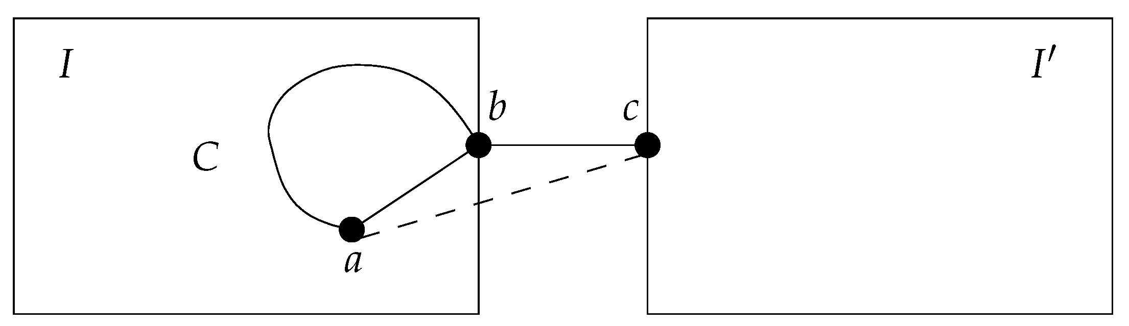
For the extreme destroyer, edge and vertex destruction are clearly more divergent from each other than for the uniform destroyer. This is reflected by our results: for edge destruction, we have a linear bound on the social cost of SE, while for vertex destruction, we have a super-linear lower bound and no upper bound at this time. The lower-bound example clearly does not work for extreme edge destruction, as explained in Remark 2. The difficulty with extreme vertex destruction is that already swapping a single leaf can have profound effects on the destroyer’s probability measure. That is, if a leaf
a swaps its one edge
for an edge
, then the number of components when
c is destroyed increases. This can lead to
c becoming the only max-sep vertex in the new graph. This signifies a drastic change, provided that before the swap, there were many max-sep vertices in different parts of the graph. It should be noted that we have no lemma saying that max-sep vertices are distributed in a certain pattern in the graph, whereas for edge destruction, it is known that they form a star-like structure ([
2], Proposition 9.1).
2.2. Open Problems
We have extensive experimental evidence and indications on the theory side that our structural result for the extreme vertex destroyer (that there is no SE tree with only one max-sep vertex for
) can be extended in two ways. We conjecture for
:
- (i)
There is no SE graph under extreme vertex destruction with only one max-sep vertex (this extends our result for trees to general graphs).
- (ii)
There is no SE graph under extreme vertex destruction that is a tree (this extends our non-existence result for trees with one max-sep vertex to trees in general).
Recall that we prove that unless the graph is two-connected, an SE cannot contain cycles for the uniform vertex destroyer. On the other hand, for the extreme vertex destroyer, our Conjecture (ii) would imply that an SE is only possible if we have at least one cycle. It would then be interesting to find a family of vertex destroyers, such that is the uniform destroyer and is the extreme destroyer, and the others are something suitable in between. When moving ε from zero to one, the probability measure should concentrate more and more on the max-sep vertices. It would be interesting to find out at which values of ε the situation switches from no non-two-connected SE having a cycle to each SE having a cycle. Our Conjecture (ii) would imply that it must switch an odd number of times.
Other interesting directions include:
Closing the gap between our lower bound and the trivial () upper bound for social cost of extreme vertex destruction.
Extension to edge ownerships and the asymmetric swap equilibrium.
Study of the model from [
17] under swap equilibrium or asymmetric swap equilibrium.
Study of vertex destruction under Nash equilibrium or pairwise stability as the equilibrium concept.
3. Model and Notation
Fix the number of players . All our graphs are finite, simple and undirected. The undirected edge between vertices v and w is denoted or . Denote the set of all graphs on the vertex set . We use the term player and vertex synonymously for graphs in . A swap for a graph is a triple of players , such that and . Denote the set of all swaps of G. Denote the graph that is obtained from G by removing and inserting ; we say that player a swaps her/his edge for the new edge . A cost function for assigns to each player a number . The social cost of G is . We call G a swap equilibrium (SE) if for all and for all .
Edge destruction: Let
be connected. For
, denote
the set of all
v-
w paths in
G. The relevance of
for
is:
That is, the number of those vertices where for each of them holds: in order to reach it from
v, we necessarily have to traverse edge
e. When
e is removed from the graph, then there will be exactly
vertices that
v will no longer be able to reach; we also say that those vertices are cut off from
v or that
v is cut off from them. An edge destroyer
is a map that associates with each
a probability measure
on
, that is
for each
e, and
. Given
, we define the cost for player
v in
G as:
that is, the expected number of vertices from which
v will be cut off after one edge is removed randomly according to the measure
. If
G is disconnected, cost is defined to be ∞.
The separation of an edge is the number of ordered player pairs such that the removal of e will destroy all v-w paths in G. If e is a non-bridge, then clearly . Otherwise, has exactly two components, say , and we call the minimal-component size of e. Then, . It is easy to see that .
Vertex destruction: For the vertex destruction model, the destroyer
associates each
with a probability measure on the vertices of
G, that is
for each
, and
. We define the destruction of a vertex not as its removal from the graph, but as the removal of all of its incident edges. This is reflected by the following definition of relevance and cost. The relevance of
for
is:
Note that since
v is in every
v-
w path, we have
, which is exactly the number of vertices that will be cut off from
v if all edges incident with
v are removed. Given a vertex destroyer
, we define the cost for player
v in
G as:
Again, a disconnected graph induces infinite cost for each player.
The separation
of a vertex
is the number of ordered player pairs
such that the removal of
u will destroy all
v-
w paths in
G. It is again easy to see that
. Moreover, if removal of
u creates
k components (not counting
u itself) of sizes
, we have:
When the graph G is clear from context, we omit the G subscripts or arguments. When a graph is defined, we write , , , etc., instead of , , , etc., respectively. The same goes for .
For any connected graph
, we call
an island if it is inclusion-maximal under the condition that the induced subgraph
is bridge-free (it does not matter whether we mean bridges of
G or bridges of
). The bridge tree
of
G is obtained by collapsing each island
I of
G to a single vertex
and inserting an edge between
and
if and only if an edge runs in
G between a vertex of
I and a vertex of
J. Obviously,
is a bijection between the set of bridges of
G and the set of bridges of
, and we will often identify those two sets. We refer to [
2] for a more formal treatment of the bridge tree.
We will also use the better-known block-cut-vertex tree; see, e.g., the book by Diestel [
22] for a definition.
4. Uniform Edge and Uniform Bridge Destruction
Denote
the set of all of the bridges of
and:
the set of bridge swaps (the case that
is disconnected is not interesting since such a swap can never bring an improvement). Clearly,
for each
.
An edge destroyer is called the uniform edge destroyer if for each and each . It is called the uniform bridge destroyer if for each and for each , for each (if , the graph is two-edge-connected, and we can take any probability measure for since the cost for each player is zero in any case).
In order to point out what are some of the essential properties of those destroyers, we look at more general destroyers first. Consider the following condition on a destroyer:
This means that if after a bridge swap an edge maintains its separation, then it also maintains its probability. This clearly includes the uniform edge destroyer and the uniform bridge destroyer. The next proposition shows that (2) is equivalent to the following simpler condition:
This means that each edge carries its fixed probability that, in the case of a bridge, sticks to it even when it is swapped for another edge.
Proposition 1. (2) and (3) are equivalent.
Proof. It is clear that (3) implies (2). Therefore, let be a destroyer with property (2). Let and . Since , we have ; hence, . Now, consider the special case first that is a path in the bridge tree. Then, the only separation that changes due to s is that of . Since separations of all other edges are maintained, they also maintain their probabilities. Since all of the probabilities add up to one, the edge also maintains its probability. In the general case, we have a path . Conducting the sequence of swaps gives the graph , and in each step, the edges maintain their probability. ☐
The following proof uses the basic idea from ([
5], Theorem 1).
Lemma 1. Let be a destroyer with property (3). Then, the bridge tree of an SE with respect to has a diameter at most two.
Proof. Let G be an SE, and for contradiction, assume that is a path in its bridge tree. Denote the number of vertices in the subtrees rooted at and d, respectively; hence, . Consider the swap . By (3), we have , and all of the other edges maintain their probabilities, as well. We have , and for all of the other edges, from the view of a, the only relevance that changes is that of , namely from to . Since G is an SE, this means . Likewise, we consider the swap and obtain . Together, this implies , which is impossible. ☐
Theorem 1. Let G be an SE for the uniform edge destroyer. Then, G is bridgeless or a star; hence, .
Proof. If
G is bridgeless, then
. Therefore, assume that
G contains a bridge. We want to show that
G is a tree, so for contradiction, assume that
G is not a tree. Let
I be an island containing a cycle, and let
be a bridge with
(and
for some island
). Then, there is a cycle
C in
I that traverses
b. Choose
a so that
. Then, the swap
puts the bridge
on a cycle and makes it part of the island, so its relevance for
a drops from a positive value to zero. No new bridges are introduced, and the relevance of all other edges remains the same for player
a. Hence, this is an improving swap, a contradiction to SE. The situation is depicted in
Figure 1.
Since we know that G is a tree, G coincides with its bridge tree. By Lemma 1, . Since , we conclude that G is a star. It follows that . ☐
Theorem 2. Let G be an SE for the uniform bridge destroyer. Then, G is bridgeless or is a star, where each of the outer islands has exactly one vertex2.
Hence, .
Proof. If G is bridgeless, then . Therefore, assume that G contains a bridge. By Lemma 1, is a star. Let I be an island that is not the center of the star (i.e., it is an outer island) and that contains more than one vertex. Then, I contains a cycle. By a swap as in the proof of Theorem 1, the one bridge e between the center of the star and I can be put on a cycle. For the players in I, this is a strict improvement since for them, e had the strictly highest relevance of all bridges in G. The statement on the social cost follows since only one vertex can be separated from the rest of the graph by the removal of a bridge. ☐
5. Extreme Edge Destruction
For
, denote
and:
We call the edges in the max-sep edges. Recall and note that is strictly increasing on ; hence, for all . Moreover, if for some and , then . In other words: exactly all of the edges with maximum are max-sep.
An edge destroyer is called the extreme edge destroyer if for each and for each .
Theorem 3. Let G be an SE under the extreme edge destroyer. Then, G is bridgeless or is a star, where each of the outer islands has exactly one vertex. Hence, .
Proof. The expression for the social cost follows from the structural statement. Assume for contradiction that G contains bridges and is not of the stated form.
Case 1:
with
. This situation is depicted in
Figure 2. By ([
2] Proposition 9.1), the max-sep edges form a star in the bridge tree. For each
, denote
the (unique) minimal component of
, and denote
the island at the center of the star formed by
. Then,
and
for all
. By assumption,
for each
i.
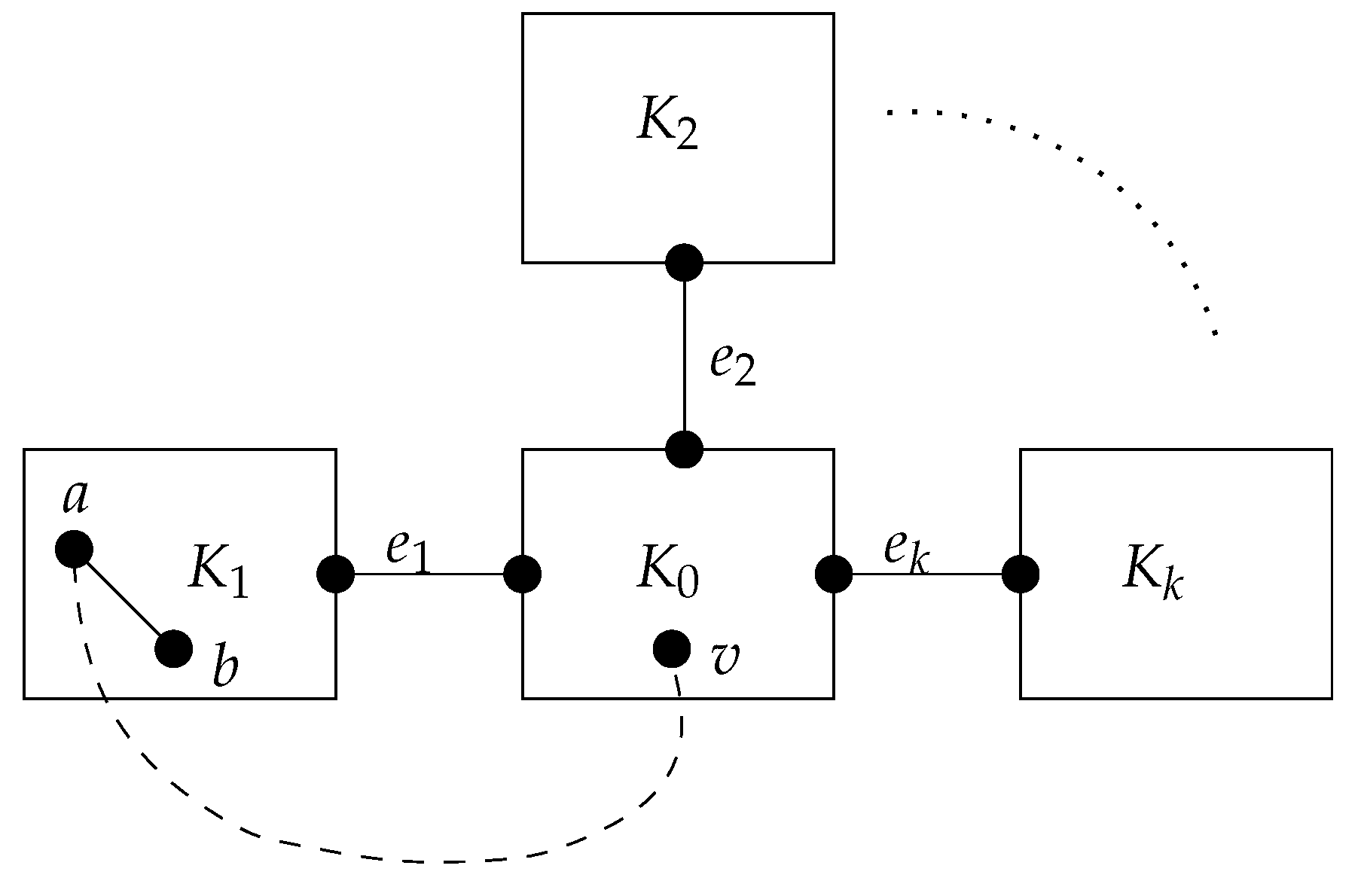
Case 1.1: There is a leaf . Denote b the neighbor of a, and let . Define . When moving from G to , all of the edges , and the edges in have their separation maintained. Edges in have their separation maintained or reduced since their minimal-component size reduces. The edge has its separation reduced since its minimal-component size reduces. The new edge cannot become max-sep since while . It follows that . We have for all . Hence, , a contradiction to SE.
Case 1.2: There is a cycle C in . Let and . By essentially the same arguments as in Case 1.1, we show that player a improves by the swap .
Case 2: . This case is more difficult since after reducing the separation of , we have no other max-sep edges that could act as a reference. Denote a component of with minimum size (if both components of have the same size, then pick one arbitrarily), and denote the island containing the endpoint of that is not in .
Case 2.1: There is a leaf . Denote b the neighbor of a, and let . Define . We have , so has the next lower possible value below . Hence, for zero or more additional edges . Since they all have the same minimum-component size, they cannot be in ; hence, they form a star with as the center (this is the only way that they can form a star in the bridge tree). If , then ; hence, the swap is an improvement. If , then ; so and . Moreover, . It follows that . On the other hand, . If or , this implies an improvement. The remaining case of and is impossible, since for such n, the graph is a star, and thus, .
Case 2.2: There is a cycle C in . We consider a swap like the one in Case 1.2. It is not difficult to see that for each ; hence, the swap is an improvement. ☐
6. Uniform and Degree-Proportional Vertex Destruction
A vertex destroyer is called the uniform vertex destroyer if for each and each .
For any connected graph , denote the set of its blocks and the set of its cut-vertices (also known as articulation points). Denote the block-cut-vertex tree of G, that is , and each edge in runs between a block and a cut-vertex, namely if and . We have for each . If , then is two-connected; we also say that B is two-connected in G. Recall also that in a two-connected graph, for each vertex v, we can find a cycle that visits v.
The following remark is proven by standard arguments, which are included here for completeness.
Remark 1. Let be any two-connected graph.- (i)
Let be three distinct vertices. Then, there exist paths and with .
- (ii)
Let with and . Then, there are with and paths and with and and .
Proof. (i) Add a new vertex
z to the graph, and connect it with
x and with
y. The resulting graph is again two-connected. Using the global version of Menger’s theorem (see, e.g., ([
22] Theorem 3.3.6)), we find two independent (that is, internally vertex-disjoint)
v-
z paths. Taking subpaths yields the result.
(ii) Let
,
be any two distinct vertices in
W. By (i), we find
and
with:
Let x be the first vertex on that is also in W. Define as a subpath of . Likewise, let y be the first vertex on that is also in W, and define as a subpath of . By (4), we get , and the other properties follow from the choice of x and y. ☐
Definition 1. Let be any graph and , , be a path in its block-cut-vertex tree . Assume , and let be a cycle in . Let . Then, we call the swap a cycle extension with respect to ; note that and are uniquely determined by the pair since is a tree.
The name “cycle extension” is chosen since the cycle C is extended into a larger cycle, thereby merging the blocks that are traversed by the new cycle. The merging property is proven in the next proposition.
Proposition 2. With notation as in Definition 1, denote . Then, in , all of the blocks are merged into one block, and the remaining blocks are maintained; in particular, no new cut-vertices emerge in , and the separation values of maintained cut-vertices do not increase.
Proof. The only non-obvious part is that is two-connected in , which we will prove now. Denote for some t. There is a cycle of the form that starts in , runs through and finally re/enters .
Let with and . Claim: in , there are paths and with and , such that and and .
Proof of claim: Denote , then . By Remark 1(ii) applied with W as defined here, the claim is clear for , since such is two-connected in (and in G). Hence, we consider . The difficulty is that may not be two-connected in , since we removed the edge . However, none of the paths P or Q guaranteed to exist by Remark 1(ii) in G can use since then, that path would have more than one vertex in common with W. This concludes the proof of the claim.
Now, let
with
. We show that in
, there are two independent
v-
w paths.
If for some , then either is two-connected and the statement is clear, or in which case , and the independent paths are given through .
Let and for . If v or w is located on , then nothing has to be done for that vertex; otherwise, we connect it with via the paths guaranteed by the claim. It is easy to see that this gives two independent v-w paths.
Let . In G, we find two independent v-w paths P and Q in . At most, one of them, say P, uses . Instead of using that edge, we can, starting at , run along until we reach a. That -a path runs outside of (except for a and ) and, thus, will not interfere with P or Q. ☐
Theorem 4. An SE for the uniform vertex destroyer is two-connected (that is, it has only one block) or it does not contain any cycle and, thus, is a tree.
Proof. Let an SE graph be given, and assume it contains more than one block. We only need to prove that no block has a cycle, or, equivalently, that each block consists of only two vertices. Suppose for contradiction that is a block with , and let be another block. Let be a cycle extension with respect to and . By Proposition 2, it follows that , since in , removal of b cannot cut a off the one or more vertices in anymore (recall that a block always contains at least two vertices). All other relevance for a is maintained or also reduced. Therefore, we have an improvement in the cost of player a, contradicting the stability of G. ☐
Corollary 1. Let be an SE for the uniform vertex destroyer. Then, G is either two-connected or a star; hence, or .
Proof. Let G be non-two-connected. Then, by Theorem 4, G is a tree. By applying the same argument as in the proof of Lemma 1, we obtain that the diameter of G is at most two, i.e., G is a star. The social cost of star is easily computed to be . ☐
A destroyer is called the degree-proportional vertex destroyer if for each and each .
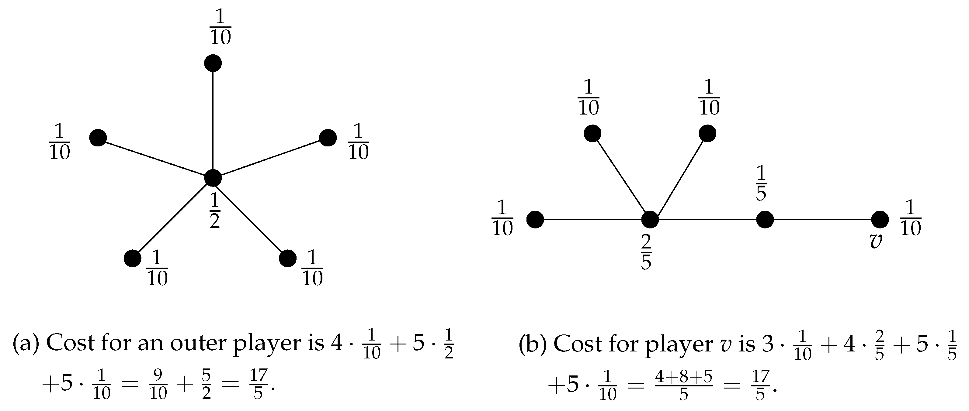
Proposition 3. The star is an SE for the degree-proportional vertex destroyer, and its social cost is .
Proof. Let
be a star. First, we prove that
S is an SE. Clearly, by just removing an edge (without creating a new one), no player can improve. It is also obvious that the only possibility for swapping is from one leaf to another leaf. Let
be leaves and
b the center of the star. Denote
. Although player
a, by the swap
, decreases the number of cut-off vertices in the case that the center
b is destroyed, this does not improve her/his cost. This is because at the same time, the degree of
c is increased, and destruction of
c in
will cut off
a from all other vertices. The following calculations show that
a indeed does not improve her/his cost by the swap. We have:
Hence,
. Therefore, the star is an SE (an example for
is given in
Figure 3). Its social cost is:
☐
Corollary 2. The social cost of SE for the degree-proportional vertex destroyer can be as high as , which is the worst possible order in the destruction model.
7. Extreme Vertex Destruction
This model is defined similarly to the extreme edge destruction model. Denote the set of max-sep vertices and . The extreme vertex destroyer picks the vertex to destroy uniformly at random from .
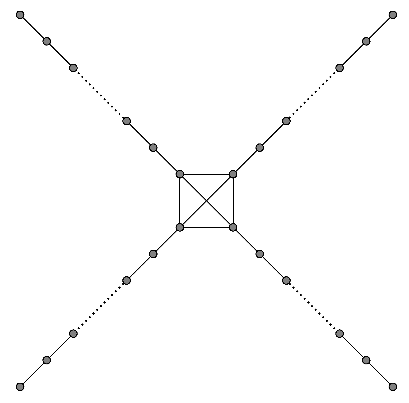
We start with a first step toward understanding the worst-case order of social cost of an SE in this model, by giving an SE example with super-linear social cost, namely
. The construction is shown in
Figure 4. It is unknown at this time whether there is a matching upper bound. Before reading the proof of the following theorem, the reader is encouraged to take look at Remark 3 in order to obtain an idea why we have to limit the length of the paths attached to the clique.
Theorem 5. Let and . Let be the graph consisting of a clique C on t vertices, and to each vertex of C, there is a path of length k attached (so, ). Then, G is an SE with .
Proof. For each player
v at distance
from
C, we have:
Since
and since the function
is strictly increasing on
, separation is strictly largest when
, that is when
. It follows
and:
If we choose
k maximal, that is
, we get:
Now, for this k, we have ; hence, . It follows (in short: we have ; if we choose k maximal, then ; hence, ).
We prove the SE property. Just removing an edge (without building a new one) is clearly not an option for the players on the paths. For a player of the clique C, nothing changes when removing an edge, since because of , the set C remains two-connected.
For , denote the k vertices on the path attached to u (note that ). In the following, whenever we consider a swap, by , we refer to the graph we obtain from G by applying the swap.
We start with the different swaps available to a player
. We have
for each
; hence:
- (i)
Consider a swap
with
and
for
, that is player
a swaps an edge from the clique to some path, but not the one connected to
a itself. Since
, the set
C remains two-connected. Separation of
u and of some vertices in
is reduced. All other separations are maintained. It follows:
Hence, the swap is no improvement for player
a.
- (ii)
Consider a swap with and , that is player a swaps an edge from the clique to its own path. Again, since , the set C remains two-connected. The separation values on some vertices in decrease, but that does not change the set of max-sep vertices, nor their relevance for a. Hence, player a’s cost is maintained.
- (iii)
Consider a swap
with
; then, in order to keep the graph connected, we have
. That is, player
a swaps the first edge on its path to some vertex on that path. We only have to exclude that
c becomes max-sep; if we achieve that, then, we know that
a’s cost is maintained. Let
be the distance between
a and
c. Then, by (1):
The latter is true by the restriction on
k in the statement of the theorem. In this computation, we used again that the function
is increasing on
.
We continue with the swaps available to a player
for some
.
- (iv)
Consider a swap with . Then, with ; since otherwise, the graph would become disconnected. From a computation like in (iii), it follows that this swap cannot make c max-sep. Hence, the cost of player a does not change.
- (v)
Consider a swap with . If , then again, a’s cost will not change. If , then c will become the only max-sep vertex in the new graph, clearly increasing a’s cost.
Now, let
for some
, that is some vertices migrate from
u’s path to
w’s path. Separation of
w and separation of the vertices
with
will increase. All other separations are reduced or maintained, so we have
. In the best case,
k vertices migrate to
w’s path; only
w becomes max-sep, and
. In this case:
Hence, the swap is no improvement for player
a. ☐
Remark 2. The graph in Theorem 5 is no SE for extreme edge destruction.
Proof. The max-sep edges are the edges on the paths that have one endpoint in the clique. This will not change when a leaf swaps to the clique; hence, this leaf will experience an improvement. ☐
Remark 3. The graph in Theorem 5 is no SE if , that is if k is larger than the upper bound in the theorem.
Proof. Let
and
b be her/his neighbor in
. Let
be at distance
l from
a, to be specified later. Denote
. If
c becomes max-sep in
, then player
a’s cost will decrease, since
, whereas the relevance of a max-sep vertex in
G for
a is
or
. By the computation in Theorem 5(iii), we see that
c becomes max-sep if
. We have:
For odd
and
, we have:
For even
and
, we have:
☐
In the remainder of this work, we provide more insight into the structure of tree SE graphs for the extreme vertex destroyer. The next theorem says that in a tree with only one max-sep vertex (and ), there is always an improving swap, so it cannot be an SE. The main concepts are that having a single max-sep vertex makes the destroyer very predictable and that swapping to a leaf, that leaf (which will have degree two in the new graph) can become max-sep only under specific conditions.
Theorem 6. There is no SE tree with , provided that .
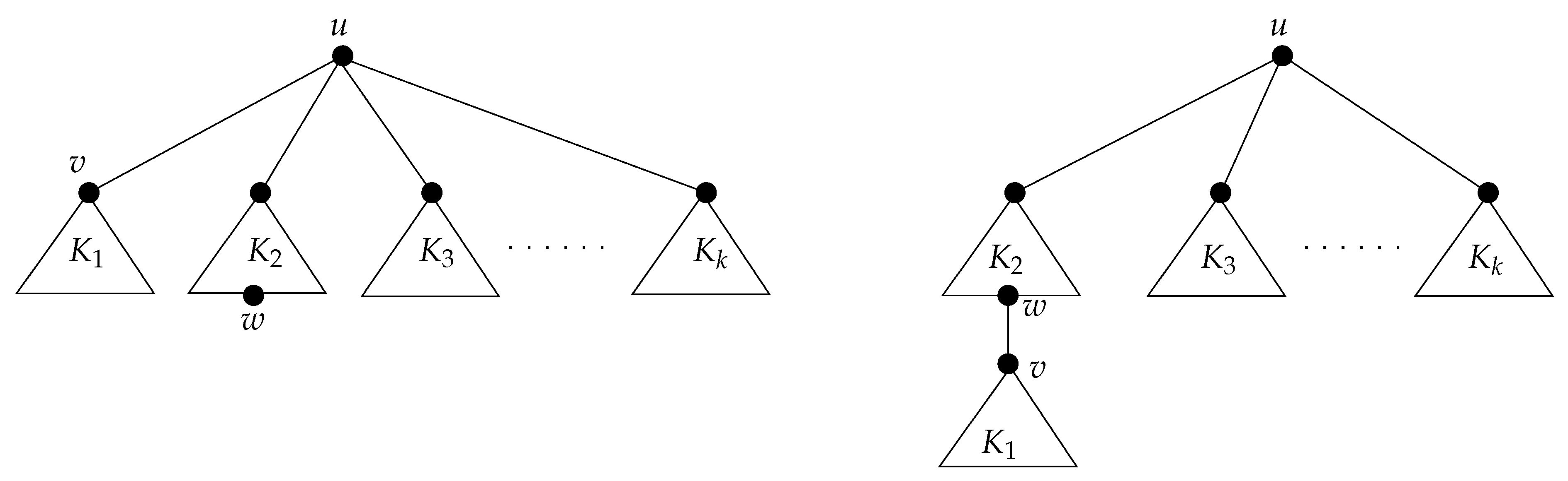
Proof. Let be an SE tree with and . It is clear that u is a cut-vertex, otherwise G is two-connected, and thus, . Denote , with , the components of ordered by non-decreasing sizes . For convenience, denote for each i.
Let
and
and
with
. We consider
, that is we detach
from
u and re-attach it to a leaf of
. The situation is depicted in
Figure 5.
Then,
and
for all
, and so, we have an improvement for
v whenever
contains at least one vertex distinct from
w. The latter is the case if
. Using (1), we compute:
Now, Condition (∗) is true if , since .
Hence, we may assume that
. Let
x be the only vertex in
. If
, then:
The last step is true since
. We conclude that
. Since
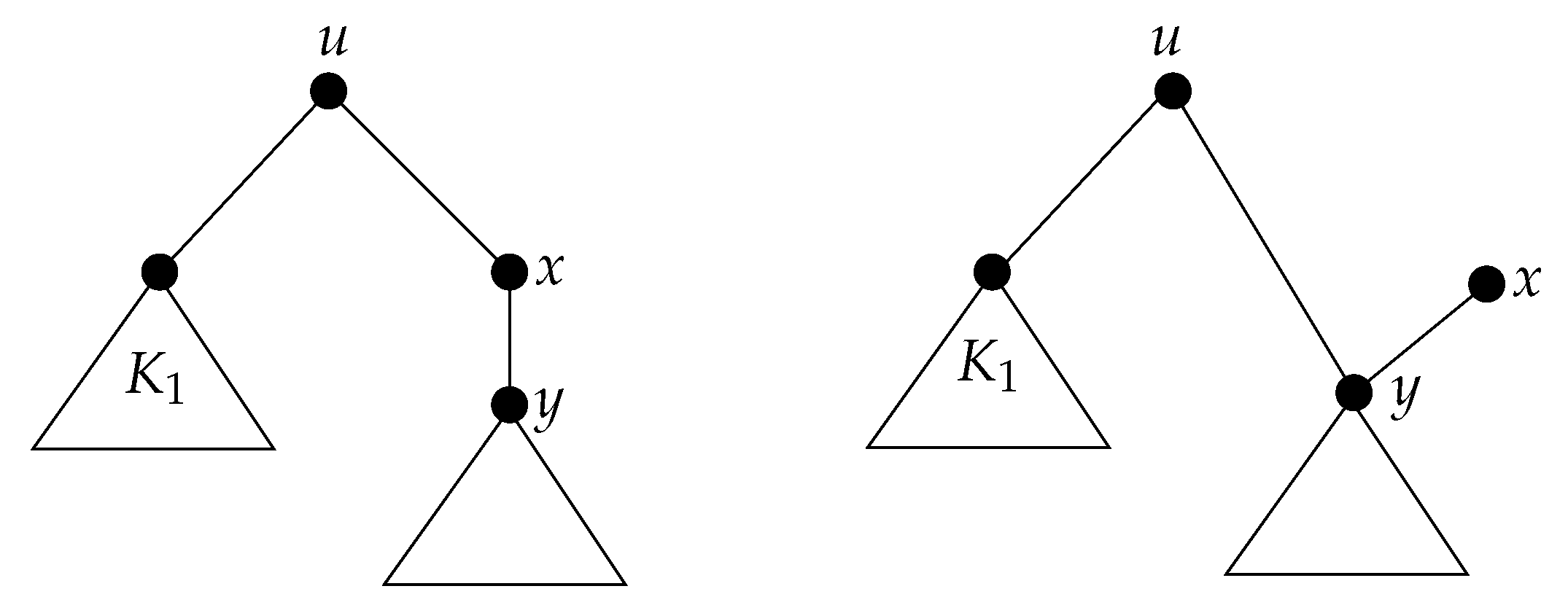
, there is
with
. We consider
, as shown in
Figure 6. We have:
Since the last statement is true, we know that ; hence, . ☐

