4.3.1. Stable Games
We now state formally the motivating connection between stable games and passivity. Let denote locally Lipschitz X-valued functions over , and denote locally Lipschitz -valued functions over .
Theorem 4.3 A stable game mapping to is δ-anti-passive, i.e.,Furthermore, if F is strictly stable, then the mapping is input strictly δ-anti-passive, i.e., for some , Proof. By definition,
δ-anti-passivity follows from negative definiteness of the integrand. Furthermore, if
F is strictly stable, there exists a
such that
which implies the desired result. ☐
In identifying stable games as
δ-anti-passive systems, we see that evolutionary dynamics that are
δ-passive are the complement of stable games in that the stability Theorems 4.1–4.2 are applicable for any
δ-passive dynamic. Inspecting the definition for
δ-passivity, we will require that for some
α,
Since this equation holds for all
, it implies a long run correlation between the
flow of population state with the flow of payoffs, namely,
4.3.2. Passive Evolutionary Dynamics
We now examine evolutionary dynamics from the perspective of
δ-passivity. A general form for evolutionary dynamics is
which describes the evolution of the strategy state,
, for the population game
F. From a feedback interconnection perspective, an evolutionary dynamic describes how strategy trajectories evolve in response to payoff trajectories. Accordingly, we will remove any explicit game description and write
In terms of previous discussions, the payoff vector
p is an “input” and the strategy
x is the output. Again, in establishing that an evolutionary dynamic is
δ-passive, we do not assert that
. Rather,
is drawn from a class of trajectories. Since stable games are
δ-anti-passive as mappings from
to
, we are interested in conditions for an evolutionary dynamic to be
δ-passive as a mapping from
to
. Specializing the definition of
δ-passivity for state space systems to the current setup, we seek to find a storage function
such that
for all admissible
. Once the above equality is established, then one can employ Theorems 4.1 and 4.2 to make conclusions about stability.
We will focus specifically on so-called excess payoff target (EPT) dynamics [
9,
19]. These dynamics form a class of evolutionary dynamics that contain several well studied cases.
First, define the
excess payoff function
by
where
is a vector of ones. EPT dynamics take the form
where
is called the
revision protocol (see [
9] for a thorough discussion.). Following [
9], we make the following assumptions:
positive correlation: .
integrability: for some function .
Finally, let
denote the subset
where
denotes the euclidean norm on
.
Theorem 4.4 For any , EPT dynamics are δ-passive as a mapping from to with storage function for some constant C.
Proof. Following [
9], take as a candidate storage function,
From integrability of
τ,
where the last inequality is due to non-negativity of
τ and positive correlation.
The remainder of the proof resolves a technicality that defines storage functions to be positive. Set
Then
is non-negative for all
and
. ☐
The proof closely follows the stability proof in [
9] that establishes
as a Lyapunov function. This resemblance should not be surprising, in light of Theorem 4.2, which establishes that the sum of the storage functions in a feedback interconnection is non-increasing.
An important difference here is that the proof does not specify the origins of the payoff trajectory. That is, we do not presume that for some stable game. Accordingly, the established δ-passivity will have stability implications for “generalized” stable games (see forthcoming sections).
The above proposition also establishes that EPT dynamics are
δ-passive as an input–output operator. In particular, since
p is the “input” and
x is the “output”,
One can construct a suitable passivity constant
α by maximizing over
,
,
, and
, as in the construction of
C.
It also is possible to establish
δ-passivity for other learning dynamics considered in [
9]. As in the case with EPT dynamics, the proofs parallel previous stability proofs in [
9], but with new interpretations with broader implications. The only subtlety is that, as before, we do not associate
in the process of establishing passivity.
We illustrate this argument for so-called impartial pairwise comparison dynamics, which are not of the EPT form [
9]. First, define Lipschitz continuous switch rates
with the property that
Impartial pairwise comparison dynamics are defined as
The interpretation from [
9] is that the flow from strategy
i to
j depends on the relative payoffs,
and
. Furthermore, impartiality means that the flow rate,
, only depends on the destination (and not origin) strategy.
Theorem 4.5 Impartial pairwise comparison dynamics defined by Equation (67) are δ-passive as a mapping from to . Proof. Following [
9], take as a candidate storage function
The derivative is
Note that we do not take
.
Arguments in [
9] establish that the summation of the first term satisfies
Rearranging the summation of the second term,
Therefore,
as desired. ☐
4.3.3. Dynamically Modified Payoffs
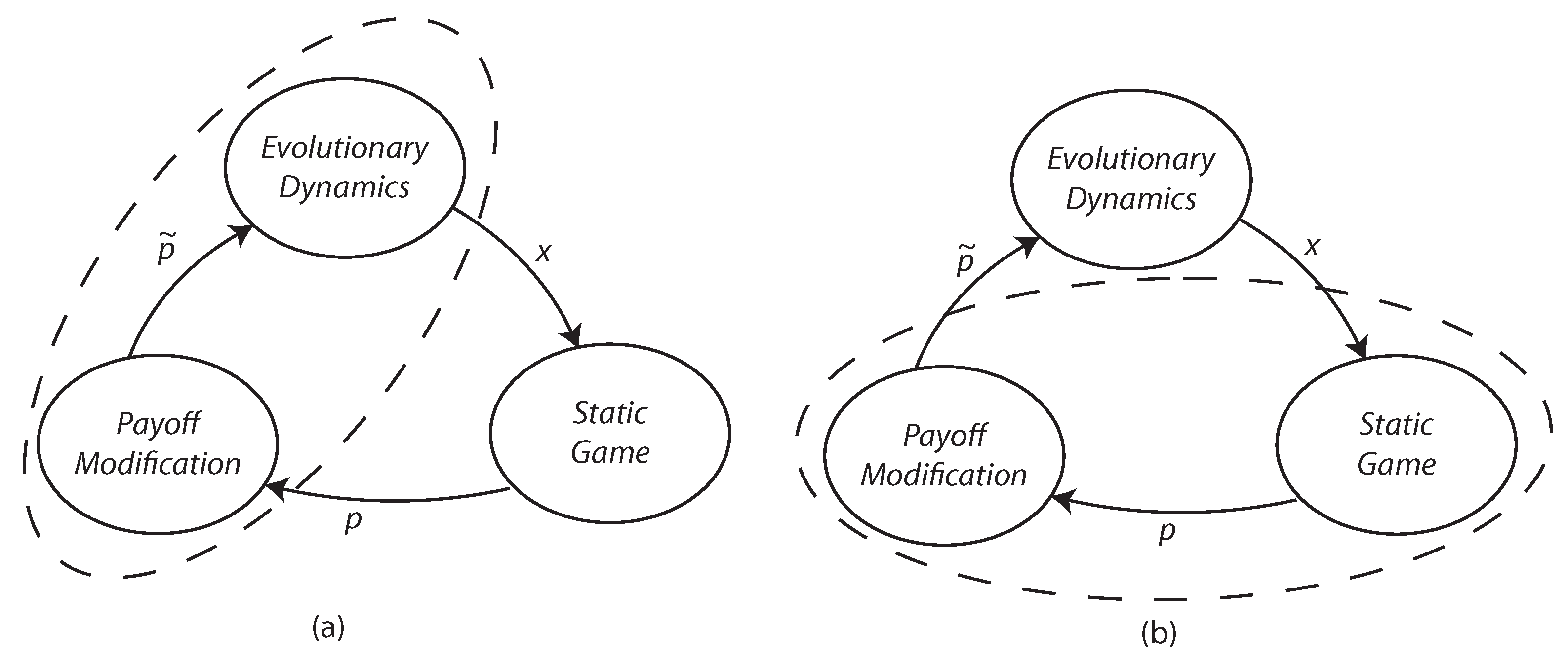
We now illustrate how passivity methods can be used for the analysis of evolutionary dynamics with auxiliary states. In this section, we consider evolutionary dynamics acting on dynamically modified payoffs. These modifications can be interpreted in two ways: (i) dynamic modification as part of an evolutionary process coupled with a static game, or (ii) a game with dynamic dependencies coupled with a standard evolutionary dynamic.
Figure 3 illustrates these two perspectives. In either case, the interconnection, and hence analysis, remains the same.
A consequence of dynamic modifications is the introduction of auxiliary states other than the strategy states. This setting is a departure from much of the literature on evolutionary games, which, almost exclusively, considers evolutionary dynamics whose dimension equals the number of strategies. Likewise, game payoffs typically are static functions of strategies.
Throughout this section, the stable games we consider are affine functions the state, i.e.,
where
A is symmetric negative definite.
Smoothed payoff modification: Payoffs are subject to an exponentially weighted moving average. Given a payoff stream
, the smoothed payoffs are
Figure 3.
(a) Static game with dynamically modified evolution. (b) Standard evolution with dynamically modified payoffs.
Figure 3.
(a) Static game with dynamically modified evolution. (b) Standard evolution with dynamically modified payoffs.
An effect of the averaging is to smooth out short term fluctuations in order to isolate longer term trends.
In state space form, the mapping from strategies to modified payoffs is described by
Theorem 4.6 The state space system Equation (77) is δ-anti-passive as a mapping from to . Proof. Take as a candidate storage function
Then
where the last inequality is due to the negative definiteness of
A. ☐
An implication of Theorem 4.6 is that Theorems 4.1 and 4.2 are now applicable for any δ-passive evolutionary dynamic coupled with smoothed payoffs of an affine stable game.
Anticipatory payoff modification: In anticipatory payoff modification, payoff streams are used to construct myopic forecasts of payoffs. Evolution (or learning) then acts on these myopic forecasts rather than the instantaneous payoffs. The concept is inspired by classical methods in feedback control as well as the psychological tendency to extrapolate from past trends. Anticipatory learning was utilized in [
3,
20,
21], where it was shown how anticipatory learning can alter the convergence to both mixed and pure equilibria.
The state space equations for anticipatory payoff modification are
Here, the modified payoff is a combination of the original payoff and an estimate of its derivative, i.e.,
The specific estimate of
here is
(see the discussion in [
20]), which can be constructed from payoff measurements. The scalar
k reflects the weighting on the derivative estimate.
Theorem 4.7 The state space system Equation (83) is δ-anti-passive as a mapping from to . Proof. Take as a candidate storage function
Then
By definition,
Therefore,
Using the above equation for
results in
where the last inequality is due to the negative definiteness of
A. We see that rescaling
leads to the desired result. ☐
The proof of Theorem 4.7 reveals that the associated dissipation inequality is satisfied
strictly because of the two terms involving
A. In particular, the anticipatory payoff modification of Equation (
83) defines an input strictly
δ-anti-passive system. The following representative theorem is then an immediate consequence of Theorem 4.1.
Theorem 4.8 In the positive feedback interconnection defined by Equation (33) (as in Figure 2b), let be any δ-passive evolutionary dynamic mapping payoff trajectories to state trajectories , and let be anticipatory payoff modification defined by Equation (83). Then . In case the evolutionary dynamic has a state space description (e.g., EPT), one can use Theorem 4.2 to conclude .
Implicit in the above discussion is that convergence of has implications about convergence to Nash equilibrium. Any such conclusions are specific to the underlying evolutionary dynamic.
4.3.4. Contrarian Effect Payoffs
In this section, we illustrate the use of passivity methods in the presence of lags or time delays. In this model, players perceive advantages in avoiding strategies that have seen net increase in recent usage. In particular, for a fixed lag
, payoffs are given by “contrarian effect” payoffs, defined by
where
is a diagonal scaling matrix. We assume that strategies are initialized by some Lipschitz continuous
, so that for
,
As intended, an increase in the usage of a strategy diminishes the perceived payoff derived from that strategy. While such a contrarian effect defined here may seem simplistic, our main interest is to illustrate the analysis of delays using passivity methods.
In this section, we will deal exclusively with the input–output operator formulation of passivity. We begin by establishing the following variant of δ-anti-passivity of contrarian effect payoffs. First, define to be the restriction of to functions with .
Proposition 4.1 Let F be a strictly stable game with strict passivity constant, , i.e.,Let be Lipschitz continuous. Let be the (contrarian effect payoff) input–output operator defined by Equation (93). Thenwith . Proof. See appendix.
Proposition 4.1 states that contrarian effect payoffs satisfy a version of passivity that deviates slightly from the usual definition of δ-anti-passivity, since the associated passivity lower bound (associated with α) is and depends on the input signal, but in a bounded manner.
The following theorem now follows from arguments similar to those for Theorem 4.1.
Theorem 4.9 In the positive feedback interconnection defined by Equation (33) (as in Figure 2b), let be any δ-passive evolutionary dynamic mapping payoff trajectories to state trajectories , and let be contrarian effect payoffs defined by Equation (93) with F strictly stable. Then . Proof. Let
be the passivity constant of the
δ-passive evolutionary dynamic, so that
By Proposition 4.1, contrarian effect payoffs satisfy
Summing these inequalities leads to
which then implies that
, as desired. ☐
