1. Introduction
In linear public good games, benefits from the common pool are smaller than the benefit of keeping everything for oneself, but investments in the common pool imply efficiency gains for the whole population. In experimental studies of repeated voluntary public goods provision (see, e.g., [
1] for an early investigation or [
2] for a recent review), participants initially contribute to the common pool. However, cooperation decreases with the length of the experiment and the growing number of participants [
3].
Allowing participants to repeatedly interact in the same group,
i.e., by implementing a partner design, also allows for conditional cooperation [
4]. Participants who cooperate conditionally adjust their contributions toward the average contribution of the whole group. This “reciprocal” adjustment is not perfect, but typically favors the adjusting participant, leading to a decline in contributions over time [
5]. Several studies (e.g., [
5,
6]) report that the majority of participants resort to conditional cooperation, while a large fraction of participants free ride and a smaller fraction of them show unconditional cooperation.
A mechanism ensuring cooperation over time is sanctioning [
7,
8], where, after each period, participants are informed of the contributions of all other participants and can impose a fine on those who did not fulfill the former’s expectations.
1 However, punishment has several drawbacks in addition to its potential demand effect: (1) It is costly for both, the punishing and the punished participant (see, e.g., [
10]). (2) Some participants punish antisocial [
11] participants who contributed more than they did. (3) Punishment is affected by an imposed and usually rather extreme relationship between the costs for the punisher and the fine imposed [
12,
13]. (4) The technology of such mandatory sanctions has no analogue in the field,
2 or more specifically, individual targeted mandatory sanctions by private agents may be useful for disentangling motives, but are rather unrealistic.
These drawbacks do not apply to rewarding. Allowing to reward may also invoke a demand effect [
14,
15], where participants can transfer part of their earnings to other participants without loss of efficiency and, thereby, ensure cooperation over time. The advantages of both, punishment and rewarding, are combined in institutions in which participants can both punish and reward [
14,
15].
Rand
et al. [
15] conclude that “it is not costly punishment that is essential for maintaining cooperation in the repeated public goods game but instead the possibility of targeted interactions more generally.” In particular, they show that both punishment and rewarding with monetary transfers,
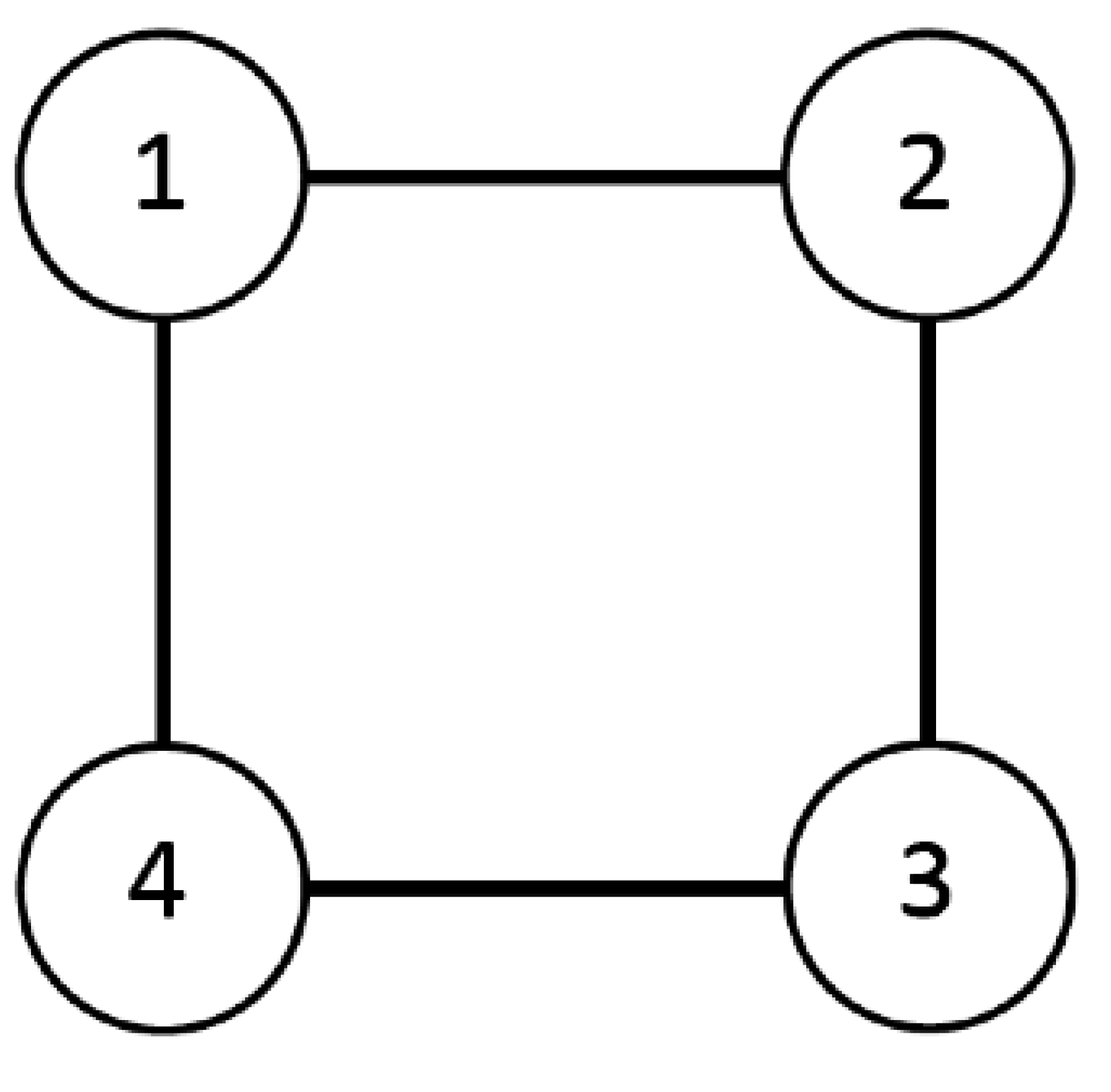
i.e., investing part of one’s income to reduce or increase the income of another participant increases cooperation. In view of this, we modify the public good game by allowing for additional targeting of contributions. Our Neighborhood Public Good Game is played by four players located at the four corners of a square. Thus, each player has two direct neighbors (at adjacent corners) and one distant neighbor. Players do not only choose their contribution, but also the location (corner) of their contribution. What a player gains from a contribution depends on her distance to the location of the contribution. It is maximal (minimal) when the contribution is located at the (opposite) position of the player. Similar to monetary transfers (as used by Rand
et al.), location choices are neutral with respect to efficiency—measured by the sum of contributions—and allow for both rewarding and punishment. For rewarding, a player locates his contribution at the position of the targeted player, while he chooses the opposite position when punishing.
Having to locate one’s contributions in one’s neighborhood is quite natural. One example is locating facilities with positive or negative external effects for one’s neighbors.
3 Furthermore, the act of locating is neither an obvious device for sanctioning or rewarding with a self-serving location,
i.e., locating one’s contribution at one’s location, as the obvious default. Will this allow voluntary cooperation by improved coordination? Since locating contributions for the whole group is efficiency neutral, this offers an intriguingly new aspect of repeated contributions in public goods experiments.
To better disentangle whether being able to locate one’s contribution fosters voluntary cooperation, we first ran treatments with endogenous location choices and then treatments in which the same location choices are exogenously imposed. Thus, any difference in behavior in the main treatments and the control treatments can be unambiguously attributed to the discretion in locating one’s contribution.
Only 16% of the participants always chose a self-serving location, confirming that they relied on location choices in spite of the self-serving location being the obvious default. Moreover, without the location option, there is less cooperation. Thus, assuming realistically that individual contributions are not just added in, but have to be located, captures a coordination device without any formal institution. In contrast to the literature on sanctioning with its demand effect [
12,
13], showing that punishment is more effective when the cost/fine ratio of punishment is low, we find the opposite effect, warning us against reaching general conclusions from strategies that employ highly unrealistic sanctioning schemes.
In
Section 2, we introduce the voluntary contribution game with its simple neighborhood structure and present our experimental design. The experimental data, comprising individual contributions and location choices, are analyzed in
Section 3.
Section 4 discusses our results.
2. Experimental Design
In this section, we first introduce the model of our Neighborhood Public Good Game and then describe our treatments and the experimental procedure.
2.1. Model
The Neighborhood Public Good Game is repeated T times. Four players () interact, and each player, , is assigned to a different corner of a square. The two players occupying adjacent corners of the square are the direct neighbors of player, i, the other player is i’s distant neighbor.
In each period, , each player, i, receives the same integer endowment, . Player i then chooses the size of the contribution, , with and its location, . Each player can locate at the position of a neighbor or his own position and keeps the difference, , for himself. The location of contribution, , can be any corner of the square, i.e., the position of one of the four players. In the following, we also refer to as the player located at corner, . Contributions have to be positive ( for all i) to make their location always payoff relevantly. Further, the contribution, , can be located at one location, , only. By allowing only positive contributions at exactly one location, we intend to understand the motivation behind the contributions. If a player could contribute nothing to the public good, his location choice would be meaningless, which we want to avoid.
The position of the player in relation to contribution,
, determines its constant marginal productivity
. For any player,
k, the marginal productivity of an individual contribution,
, is:
where
and
. The payoffs are given by:
for all players,
, and all periods,
with
for all
i and
t. Although the location of contribution,
, affects the individual gains from
, it does not influence the aggregated payoff of all players,
, as the aggregated marginal benefit of a contribution is
always.
Note that locating one’s contribution does not only target just one community member, but favors the one whose location is chosen and harms another who is at the opposite corner. In our view, this captures a usual aspect of most sanctioning devices in the field and questions individual targeting in sanctioning without external effects on others.
2.2. Treatment Design
We conducted experiments to investigate the impact of location choices. In particular, we introduced treatments varying the values,
,
and
, without changing the sum,
. Larger differences can, for instance, allow one to seriously harm the distant contact. Since we expected an increase in cooperation when participants have more discrimination power, we conducted two versions of the Neighborhood Public Good Game, Treatments,
and
, using different values for
,
,
:
In addition, we performed control Treatments, and , of the Neighborhood Public Good Treatments, and , where the location choices of participants are exogenously imposed, i.e. location choices were drawn from a uniform distribution. We did not inform participants of the control sessions how locations were determined—all the - and - instructions say is “Locations are predetermined and independent of your behavior.”
Table 1 summarizes all four treatments.
2.3. Procedure
We recruited participants using ORSEE [
16] for our computerized (using z-Tree, [
17]) experiment. At the beginning of a session, participants were randomly seated in the laboratory. We handed out
Table 1.
Distinction of treatments.
Table 1.
Distinction of treatments.
| | | Intensity of punishment/rewarding |
| | | low () | high () |
| Location | by participant | | |
| choice | by random draw | | |
written instructions (see
Appendix A for an English translation), which were also read aloud to make them common knowledge. After privately answering questions concerning the instructions, we checked the understanding of the instructions by a control questionnaire. Participants who were not able to answer these questions were replaced (altogether, 15 participants).
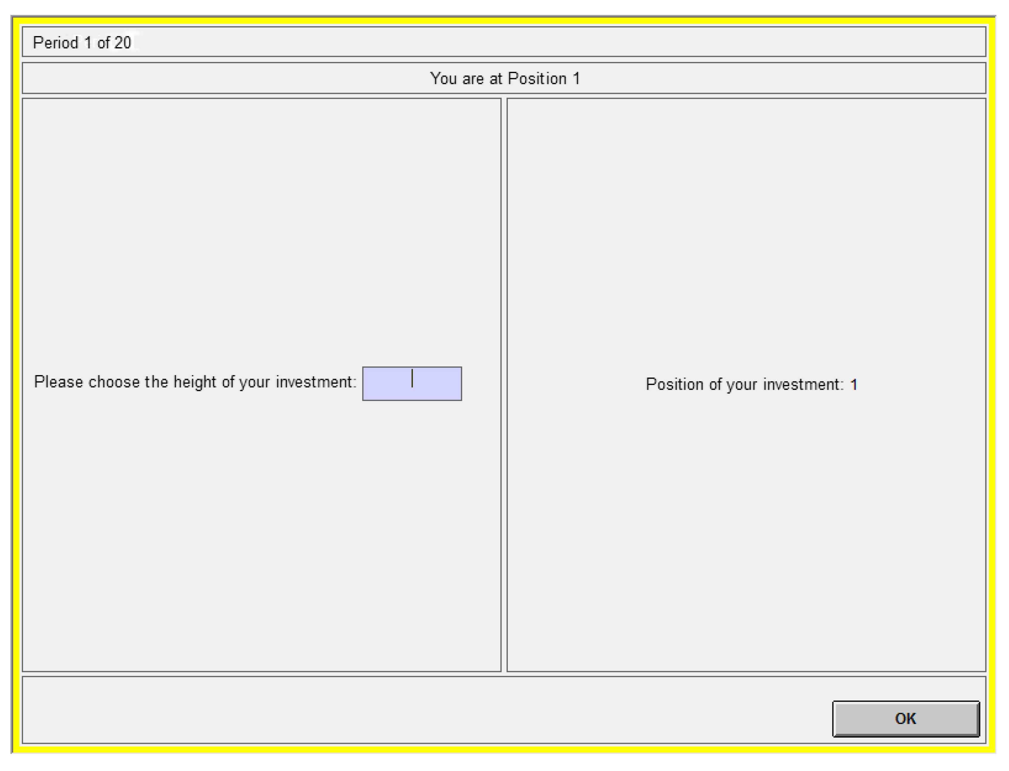
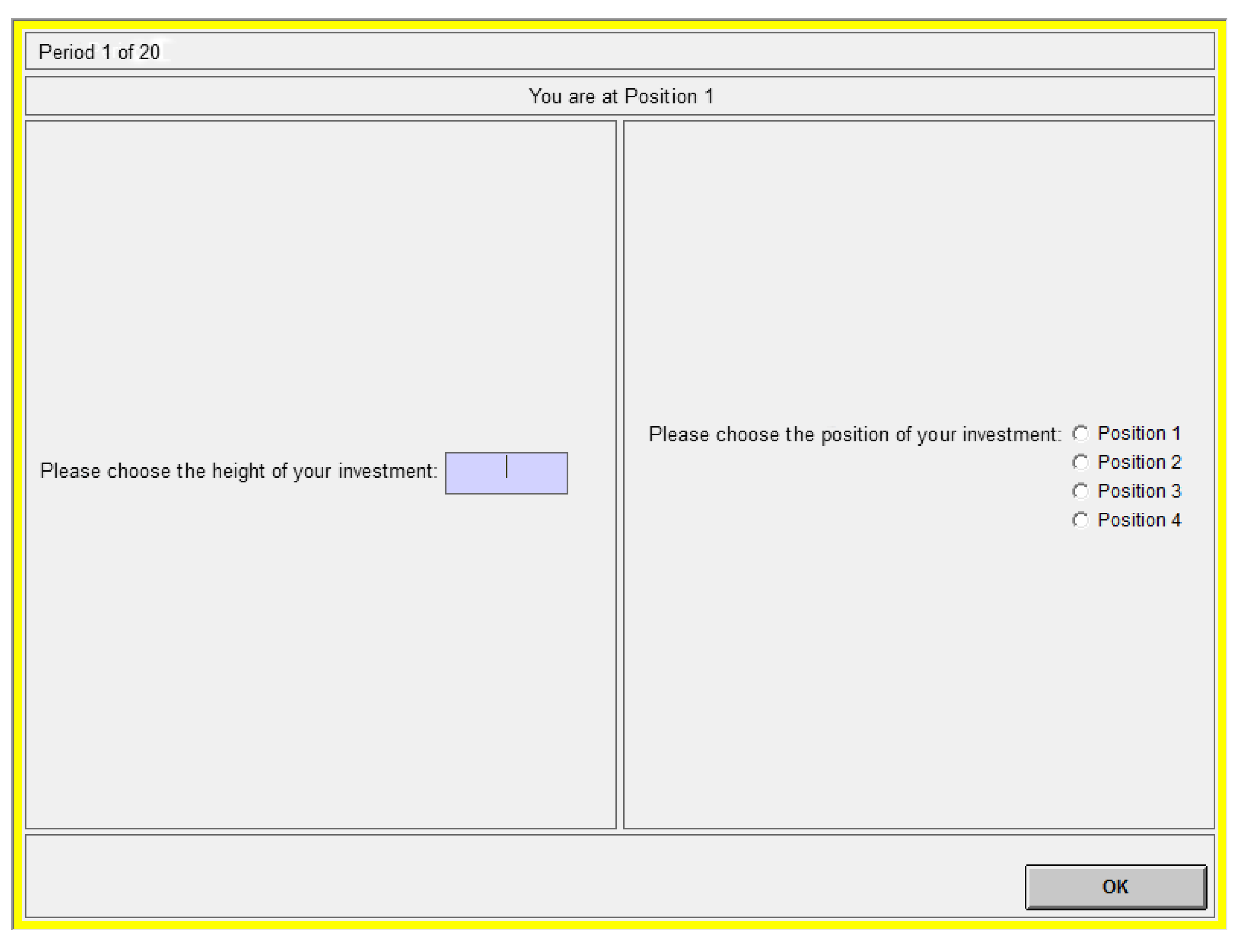
The participants played the four treatments of the Neighborhood Public Good Game for (
) 20 periods.
4 In the beginning of the first period, we assigned each participant to a group and a location, which did not change throughout all 20 periods. In each period,
t, participants received an endowment of (
) 10 tokens. Each participant,
i, decided how many tokens to contribute to the public good (
). In the
M Treatments, each participant also had to specify where to locate it (
), while participants in the
C Treatments were shown a location drawn from a uniform distribution where they could contribute. Each token was worth 10 points. Hence participants earned an integer number of points in each period, given the parameters in
Table 1. At the end of each period, we informed the participants of their payoff, the contributions,
, and the location choices,
, of all participants in the current period. No additional information concerning other participants was given.
Table 2.
Overview of treatments conducted.
Table 2.
Overview of treatments conducted.
| Treatment | Sessions | Independent | No. of |
| | No. | groups per session | observations | participants |
| 3 | 8 (Sessions 1 and 2), | 23 | 92 |
| | | 7 (Session 3) | | |
| 3 | 8 (all sessions) | 24 | 96 |
| 3 | 8 (all sessions) | 24 | 96 |
| 3 | 8 (all sessions) | 24 | 96 |
| Sum | 12 | 95 | 95 | 380 |
A session lasted 60 to 90 minutes, including 25 minutes for reading and understanding the instructions. We paid participants privately at the end of each session. They earned points as payoffs (100 points = 0.20 euro). The average payoff was 14.02 euro. A participant who was replaced after not understanding the instructions received 2.50 euro in addition to the show-up fee of 2.50 euro.
Three hundred and eighty students from various fields of study participated in the experiment at the laboratory of the Max Planck Institute of Economics in Jena. We conducted three sessions with 32 participants for each of the four Treatments (
,
,
,
) with eight groups and one session of Treatment
with 28 participants in 7seven groups (see
Table 2). Hence, we generated 24, respectively 23, independent observations per treatment. The reduction to 23 independent observations in Treatment
resulted from a hardware failure.
2.4. Hypotheses
Clearly, the solution behavior (from backward induction, e.g. in the sense of repeated elimination of weakly dominated strategies or subgame perfect equilibria) for all four players, i, is and in all periods, t. For an efficient outcome, all participants must choose and can make any location choice, , in all periods, t.
However, results from experimental investigations show deviating behavior: in the Neighborhood Public Good Game, participants interact in a partners design. Previous studies (e.g., [
18]) have shown that participants engage in initial cooperation, but reveal a downward sloping development of contributions with a further decline of cooperation in the terminal period. We expect qualitatively similar attempts for
in the Neighborhood Public Good Game, where our participants can additionally make self-serving location choices,
, but much less reliability of such attempts. In our view, this is mainly due to the unrealistic technology of individually targeted and highly detrimental monetary sanctions.
Hypothesis 1 Cooperation decreases after the first period with:- (a)
contributions decreasing rapidly over time and
- (b)
an increasing number of self-serving location choices in later periods.
The higher variance between
,
and
in the
treatment than in the
treatment allows for higher discrimination power regarding location choices. In particular, the positive behavior of others can be more highly rewarded in the
treatment. As we expect reciprocity to be the driving force behind behavior, we also expect more cooperation in the
than in
treatment.
Hypothesis 2 Participants contribute more in the treatment than in the treatment.
Finally, only in M treatments can participants reciprocate the behavior of others, while in C treatments, the location choices are randomly determined. Hence, we derive the following hypothesis.
Hypothesis 3 Participants contribute more in the M than in the C treatments.
3. Results
3.1. The Benefit of Location Choices
The overall contributions (see
Figure 1 (b))
5 in the first period are 5.73 (in
) and 5.72 (in
) and are significantly higher than the contributions of 4.30 (in
) and 4.27 (in
) without location choices (
vs. (MW): p=0.016 /
vs. (MW): p=0.003). Although contributions in treatments with location choices remain higher than contributions in treatments without location choices, they decrease at least for the first 10 periods (
vs.
(MW): p=0.007 /
vs.
(MW): p=0.016) until they approximate each other in the last period, clearly confirming Hypothesis 1 (a) (
: 3.50,
: 2.95,
: 2.41,
: 2.35). Compared to period 19, the last period only shows a weak endgame effect (in
) if any (
(WX): p=0.062 /
(WX): p=0.070 /
(WX): p=0.061 /
(WX): p=0.046).
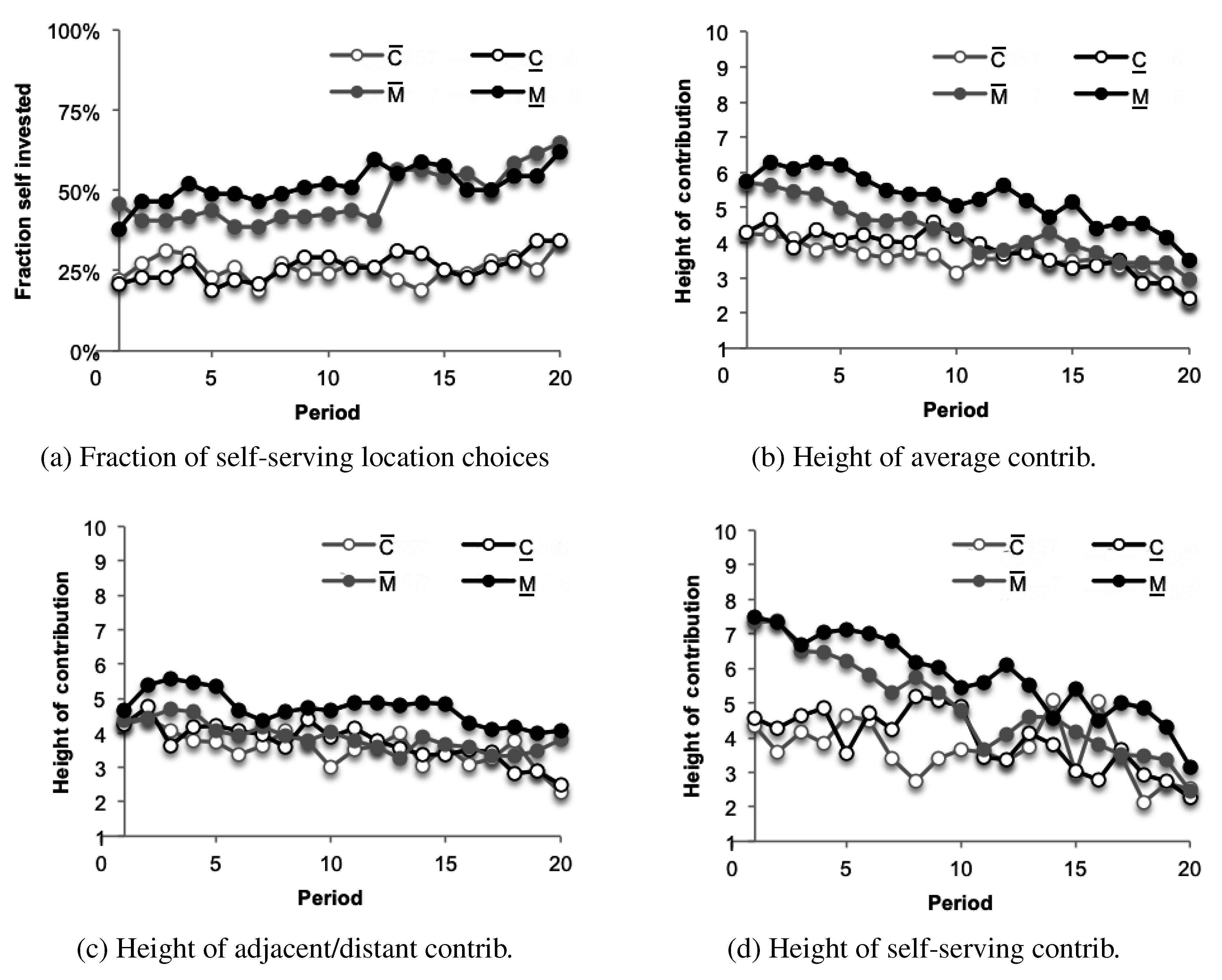
Figure 1.
Development of contributions per treatment
Figure 1.
Development of contributions per treatment
Result 1 Being able to freely locate one’s contribution fosters initial cooperation, but cannot prevent its erosion over time.
We attribute the decrease in contributions (mainly) to the increase in self-serving location choices. Both with high and low intensity of punishment or rewarding, significantly more (about 50%, see
Table 4) participants invest in their own location than in experiments with random location choices (
vs. (MW): p=0.001 /
vs. (MW): p=0.026) and the fraction of investments in self-serving locations slightly increases over time, confirming Hypothesis 1 (b) (see
Figure 1 (a)). An analysis of contributions at adjacent/distant locations (see
Figure 1 (c)) and contributions at self-serving locations (see
Figure 1 (d)) in isolation confirms this. Contributions are significantly higher in treatments with location choices, both for self-serving (
;
vs. (MW): p=0.001 /
vs. (MW): p=0.000) and other contributions (
vs. (MW): p=0.045 /
vs. (MW): p=0.013). The effect even persists during the first 10 periods for contributions in self-serving (
vs. (MW): p=0.001 /
vs. (MW): p=0.003) and other locations (
vs. (MW): p=0.029 /
vs. (MW): p=0.033).
Table 3.
Comparison of first period contributions based on location choices.
Table 3.
Comparison of first period contributions based on location choices.
| Treatment | Other locations | Own location |
| | Mean | SD | Mean | SD |
| 4.65 | 3.52 | 7.49 | 3.80 |
| 4.35 | 2.88 | 7.34 | 3.85 |
| 4.24 | 3.48 | 4.55 | 3.89 |
| 4.25 | 3.43 | 4.33 | 3.41 |
However, the effects are stronger for self-serving location choices (in
p-values). The difference between contributions at self-serving and distant location choices is most obvious when contributions in the first period are analyzed (see
Table 3). Here, contributions at other locations are, on average, around four for all four treatments. However, in treatments allowing participants to choose the location of their contribution, the average contribution at self-serving locations is about twice as high. In addition, we find no endgame effect for contributions at self-serving locations (
(WX):
p = 0.236 /
(WX):
p = 0.091 /
(WX):
p = 0.352 /
(WX):
p = 0.415). Nevertheless, there is an endgame effect for contributions at other locations for Treatment
and
(
(WX): p=0.063 /
(WX):
p = 0.095 /
(WX):
p = 0.135 /
(WX):
p = 0.018).
To sum up, contributions differ between treatments with and without location choices. This effect can be mainly attributed to the role of self-serving location choices. Whenever participants have the possibility, contributions at self-serving locations are more frequent and corresponding contributions are (at least initially) higher than choices for other locations.
Result 2 Contributions at self-serving locations compensate this effect by being larger than contributions at distant locations, suggesting one can substitute free riding by self-serving location choices.
3.2. Impact of Costs for Rewarding and Punishment
How fast cooperation decreases depends on the reward and punishment effects by location. While more than 40% of location choices fall on adjacent locations, only 5% choose distant neighbors (see
Table 4). In particular, while no significant difference between the random (Treatments
C) and the target mechanism (Treatments
M) exists for adjacent locations (MW:
p = 0.150), self-serving contributions at (distant) locations are significantly higher (lower) when participants choose these themselves (self-serving (MW):
p = 0.000 / distant (MW): p=0.000). Thus, they refrain from punishment and rewarding of distant neighbors and focus on adjacent neighbors. The difference in impacts between Treatments
and
leads to differences in the effectiveness of this mechanism.
While investments in the second half of the experiment are significantly higher in Treatment
than in Treatment
(MW:
p = 0.010), no difference exists between Treatment
and Treatment
(MW:
p = 0.359). Although the benefit of our punishment and rewarding mechanism decreases in
Table 4.
Fraction and contributions of participants investing in location types per treatment.
Table 4.
Fraction and contributions of participants investing in location types per treatment.
| | Adjacent | Distant | Self-serving |
| Treatment | Fraction | Height | Fraction | Height | Fraction | Height |
| | Mean | SD | Mean | SD | Mean | SD | Mean | SD | Mean | SD | Mean | SD |
| 43.9% | 0.257 | 4.83 | 2.07 | 4.5% | 0.054 | 3.42 | 2.74 | 51.7% | 0.272 | 5.45 | 2.56 |
| 47.7% | 0.297 | 3.00 | 1.91 | 4.5% | 0.047 | 4.03 | 2.35 | 47.8% | 0.311 | 4.41 | 2.68 |
| 49.7% | 0.067 | 4.07 | 2.35 | 24.1% | 0.060 | 3.29 | 2.41 | 26.2% | 0.050 | 3.73 | 2.18 |
| 49.5% | 0.044 | 3.82 | 2.09 | 24.9% | 0.053 | 2.92 | 2.09 | 25.6% | 0.051 | 3.67 | 2.42 |
the
Treatment, it persists until the final period (
vs.
(MW):
p = 0.013 /
vs.
(MW):
p = 0.220; U = 251.0).
An analysis of all 20 periods shows that allowing for location choices in Treatment is strongly beneficial - here contributions are significantly higher in the M treatment than in the C treatment confirming Hypothesis 3 (MW: p=0.005), while it has no positive impact on contributions in Treatment for the whole experiment contradicting Hypothesis 3 (MW: p=0.076). A side effect of this observation is that average contributions per group are significantly higher in Treatment than in Treatment , obviously contradicting Hypothesis 2 (MW: p=0.046).
Clearly, the results in this subsection are surprising, especially the low contributions in Treatment . In the remainder of this section, we analyze this unexpected behavior from different angles.
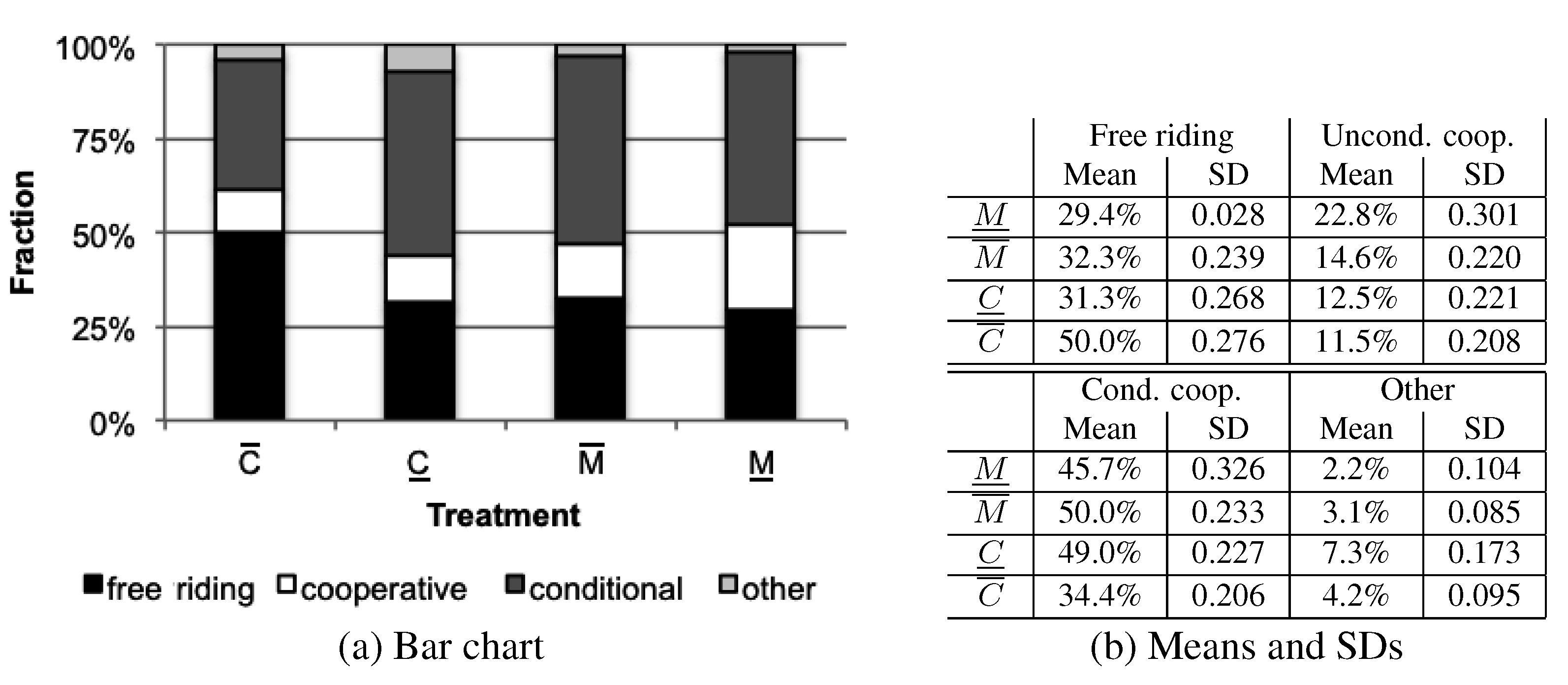
3.3. (Un)conditional Cooperation and Free Riding
To classify cooperation behavior as conditional cooperation, unconditional cooperation and free riding, we resort to a notion introduced by [
4] and formalized by [
6]. In line with this approach, we plot the contributions of each participant against the average contribution of the remaining group in the previous period,
i.e., against observed behavior. We classify participants making contributions above (below) the
line as cooperators (free riders). If the contributions of a participant cluster around the
line, we classify him as a conditional cooperator. Formally, we perform an ordinary least-squares regression of the participant’s contribution on the average contribution of the group. If the regression line is always above (below) 50% of all possible contributions, we classify the participant as an unconditional cooperator (free rider). If the regression line has a positive slope and lies both above and below 50% of all contributions, we classify the participant as a conditional cooperator. We classify all participants who do not fit any of the criteria as others. Although this approach may lead to misclassification (see [
6]), we consider it to be accurate and not prone to tendentious classifications by visual inspection.
On average, the distribution of strategies is similar to other studies on public good games. The majority of all participants (about 45%) resort to conditional cooperation. The second largest group are free riders (about 36%), the smallest group any unconditional cooperators (about 15%). Only 4% of all participants do not fall into either of these groups. When the treatments are investigated in isolation, only Treatment
is different (see
Figure 2). Here, with about 50% of all participants, significantly more participants free ride compared to about 30% in all other treatments (
vs.
(MW):
p = 0.016 /
vs.
(MW):
p = 0.011). This effect comes at the expense of the frequency of conditional cooperators. In Treatment
, only 35% of all participants resort to conditional cooperation—significantly less than the about 48% in the other treatments (
vs.
(MW):
p = 0.013 /
vs.
(MW):
p = 0.017).
Figure 2.
Fraction of contribution “strategies”.
Figure 2.
Fraction of contribution “strategies”.
We now compare contributions between all three strategies by calculating the average contribution per group for each strategy, i.e., free riding, conditional cooperation and unconditional cooperation. We then select only those groups in which participants show this behavioral pattern and compare the contributions between these groups. The analysis shows for all four treatments that free riders contribute significantly less ( (WX): obs. 12; p = 0.002 / (WX): obs. 18; p = 0.000 / (WX): obs. 17; p = 0.000 / (WX): obs. 19; p = 0.000) and earn significantly more ( (WX): obs. 12; p = 0.002 / (WX): obs. 18; p = 0.000 / (WX): obs. 17; p = 0.000 / (WX): obs. 19; p = 0.000) than conditional cooperators.
Result 3 Conditional cooperators suffer from the existence of free riders, which explains the decline in cooperation over time.
3.4. Punishment, Rewarding and Reciprocity
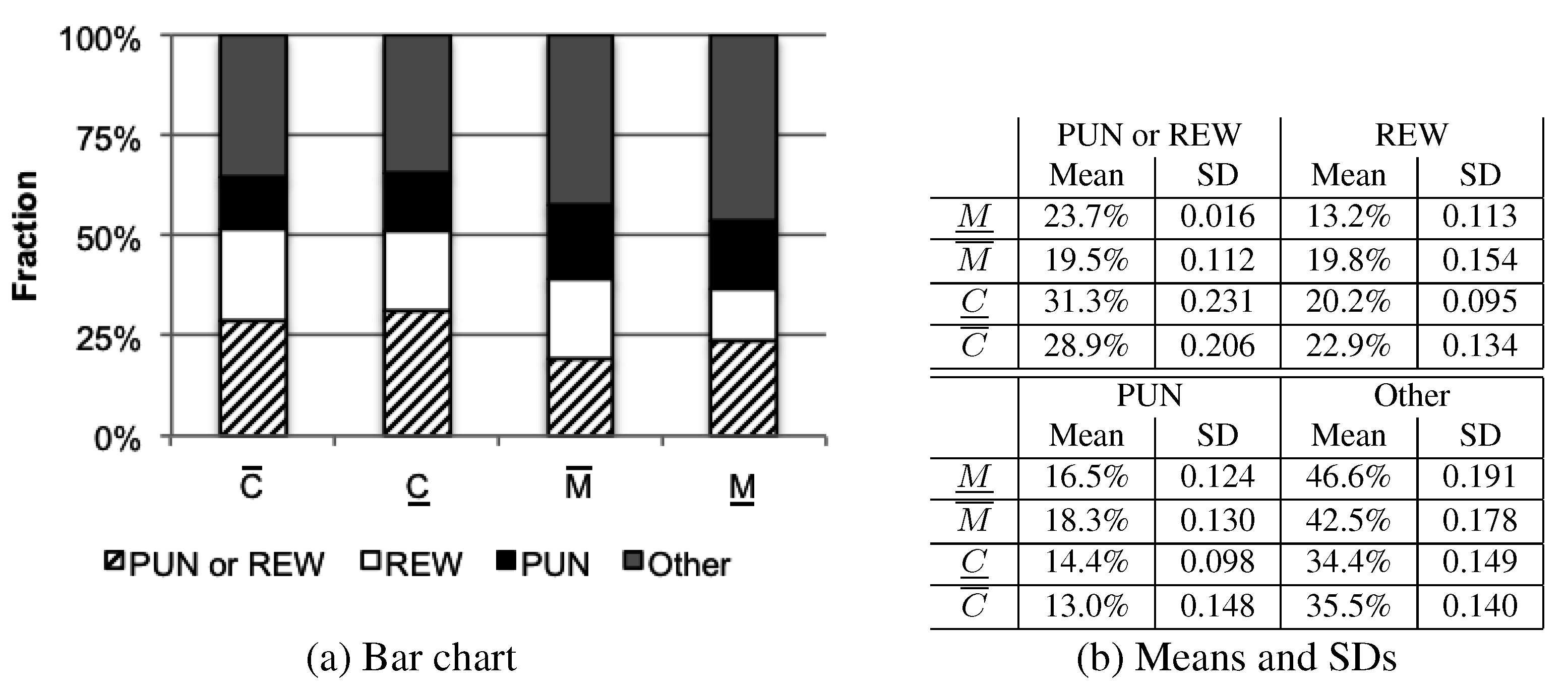
In this subsection, we analyze if location choices are used to punish or reward. To do so, we focus on all non-self-serving location choices (and classify them as punishment or rewarding for a previous act). We rank the highest contributions from the preceding period first and the lowest contributions last. If a participant chooses the participant ranked first in the preceding period as a target for his contribution, we classify this as rewarding and if she chooses the participant opposite to the participant ranked last as punishing. Notice that the first and last rank are opposite to each other, so that locating the contribution at the first rank might be both, punishment and rewarding. We capture this aspect in a third class,
i.e., “either punishment or rewarding.” All location choices which do not fit any of these criteria are categorized as “other choices.”
Figure 3 captures the classification of all our treatments.
Punishment and rewarding differs between treatments without location choices (around 30%) and treatments with location choices (around 20%). However, this difference is not significant (
vs.
(MW):
p = 0.182 /
vs.
(MW):
p = 0.061). In both
M treatments, the fraction of rewarding location choices is about 5% lower than in the
C Treatments. The effect is significant for a comparison of Treatments
and
(
vs.
(MW): p=0.016 /
vs.
(MW): p=0.106). The fraction of punishment choices is quite similar for all treatments (around 15%), although significantly higher
Figure 3.
Fraction of location “strategies”.
Figure 3.
Fraction of location “strategies”.
in Treatment
than
(
vs.
(MW):
p = 0.351 /
vs.
(MW):
p = 0.044). Hence, we believe that neither rewarding nor punishment is an important motive behind making location choices.
Result 4 Contrary to our expectations, location is not used to punish, respectively, reward, past behavior.
Table 5.
Reciprocity and location choices.
Table 5.
Reciprocity and location choices.
| Treatment | Pos. or neg. | Pos. | Neg. | No reciprocity |
| 13.3% | 29.2% | 14.9% | 42.5% |
| 16.9% | 25.6% | 19.9% | 37.6% |
| 6.8% | 18.9% | 17.3% | 57.0% |
| 6.7% | 19.3% | 18.3% | 55.7% |
Do participants use the mechanism to simply reciprocate the location choice made by others? Let us classify a location choice as positively reciprocal if a participant, after being chosen as a target, chooses the giving participant as a target in the next period. As negatively reciprocal, we classify contributions if a participant invests in the distant location of another participant and the latter reciprocates in the next period by investing in the distant location of the former.
Example: In period 1, let the participant at location 1 locate her contribution at location 2. In period 2, the participant at location 2 can show positive reciprocity by investing in location 1, i.e., the location of the initially giving participant, while the participant at location 4 can show negative reciprocity by investing in location 3, i.e., the location opposite to location 1.
As both definitions, positive and negative reciprocity, do not exclude each other, some contributions might be positively and negatively reciprocal.
Table 5 gathers the fraction of corresponding reciprocal acts for all four treatments (again, analyzing non-self-serving location choices only).
Notice that in both C treatments, reciprocity is not possible by intention, as all location choices are chosen from a uniform distribution instead of being specified by the participants. However, reciprocity (according to our definitions of positive and negative reciprocity) might occur even in these treatments. Hence, the comparison of C and M treatments is meaningful: only if reciprocity occurs more frequently in the M treatments than in the C treatments, can it be intended.
In Treatments and , 57.5%, respectively, 62.4%, of all contributions not assigned to a self-serving location are positively or negatively reciprocal (compared to around 44% in the random treatments), indicating that it is reciprocity that drives location choices in the Neighborhood Public Good experiment. For both treatments, it triggers positive reciprocity more frequently than in a random location ( vs. (MW): p = 0.016 / vs. (MW): p = 0.043). While negative reciprocity occurs less frequently in Treatment than in , no such effect occurs in Treatment ( vs. (MW): p = 0.008 / vs. (MW): p = 0.156).
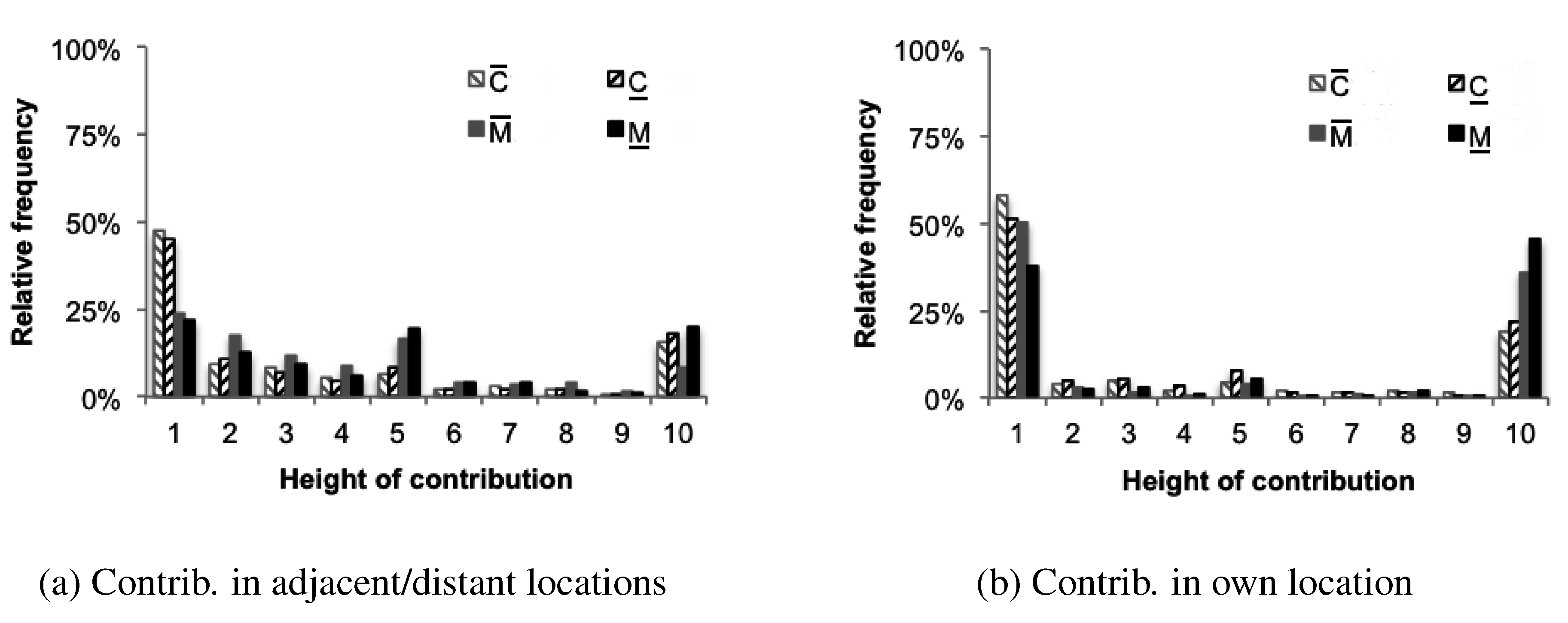
Figure 4.
Height of contributions
Figure 4.
Height of contributions
Result 5 Participants of the M treatments reciprocate the location choice by positively (negatively) reacting to others who locate (distance) their contributions from their position.
4. Discussion
We believe that in a real world, people implement different mechanisms to punish. Think of a firm, where managers can rely on the punishment mechanism often described in the economic literature (e.g., [
7,
12]), while ordinary employees cannot. Instead of cutting salaries or imposing fines, they reward and punish others by distributing or not distributing information. This approach typically incurs no cost on the punisher. However, this punishment mechanism involves a targeted effort. In this sense, we have proposed an unusual way of punishment: our subjects could punish others by locating their contributions in a specific way. We consider this approach to be realistic, not only for teams, but also for families or clubs in which an individual has only limited influence on the formation of the group. In our experimental design, by choosing whom to give new information, the participant controls who finally receives the information and at what precision—more distant participants will not get the information, while close ones will.
With our “Neighborhood Public Good Game”, we have tried to capture such situations by an admittedly stylized paradigm. We expected some initial difficulties of participants in locating their contributions, e.g., in using this action as a means to sanction or reward specific others, but that they would subsequently try to establish high and only slowly decreasing levels of cooperation and an intensive use of rewarding. Since by rewarding one participant another participant is always punished (and
vice versa), we did not expect the permanently high levels of cooperation as observed in other experiments with punishment [
7] and rewarding [
15]. However, the monetary sanctioning schemes in these studies rely on a dramatic inefficiency of sanctions, explaining why our findings are different. Other than in traditional Public Good games, participants in our experiments cannot only free-ride or cooperate; location choices provide them with a happy medium: they can invest in the group project and place their investment in a self-serving location. This is exactly how they use the mechanism. However, one would expect that in the
treatment this effect would be more obvious, as the loss between group investments in self-serving locations and keeping the money is smaller than in the
treatment. This is not the case, because only in the
treatment are contributions significantly higher than in the
treatment, indicating that being perceived as too selfish is not accepted by the participants. In addition, rather than using a location for punishment and rewarding, participants simply use the mechanism to reciprocate the location choices made by others. Nevertheless, we find that, initially, cooperation is higher in an experiment allowing for location choices than in an experiment without this option.
Table 6.
Fraction of contribution compared to endowment.
Table 6.
Fraction of contribution compared to endowment.
| | First period | Last period |
| Partner designs |
| Keser and van Winden, 2000 [18] | 57% | 10% |
| Fehr and Gächter, 2000 [8] | 56% | 16% |
| Punishment |
| Fehr and Gächter, 2000 [8] | 62% | 90% |
| Egas and Riedl, 2008 [12] | 45% | 25%-55% |
| Nikiforakis and Normann, 2008 [13] | 43%-65% | 4%-85% |
| Rewarding |
| Sefton et al., 2007 [14] | 60% | 20% |
| Rand et al., 2009 [15] | 75% | 85% |
| Our treatments |
| 57% | 35% |
| 57% | 30% |
| 43% | 24% |
| 43% | 24% |
Compared to other mechanisms (see
Table 6), allowing for location choices yields the same level of first period contributions as all other designs, namely partner designs and punishment and rewarding. However, the benefit of a mechanism can be observed only in the periods closer to the end of the game, where location choices clearly outperform the partner design with contributions being approximately twice as high in our treatments. Rewarding clearly outperforms location choices—here, cooperation in the terminal period lies above that in the first period.
6 The results concerning punishment are mixed. While the mechanism introduced by [
8] clearly outperforms location choices, experiments with higher relative costs for punishment yield results similar to ours (see [
12,
13]).
As usual, it is widespread conditional cooperation and the existence of free riding that leads to a fast and steady decrease in cooperation. The decrease is faster, the more drastic the payoff effects of location choices are.
Table 7.
Distribution of strategies compared to literature.
Table 7.
Distribution of strategies compared to literature.
| | Free Rider | Cooperator | Cond. coop. | Others |
| Fischbacher et al., 2001 [4] | 30% | 14% | 50% | 6% |
| Kurzban and Houser, 2005 [6] | 20% | 13% | 53% | 14% |
| Chaudhuri and Paichayontvijit, 2006 [19] | 16% | 16% | 62% | 4% |
| 29% | 23% | 46% | 2% |
| 32% | 15% | 50% | 3% |
| 31% | 13% | 49% | 7% |
| 50% | 12% | 34% | 4% |
The strategies observed are similar to existing experiments on repeated Public Good Games using the partner design (see
Table 7), both in the types observed and their frequency. Given our expectation that location choices should allow for punishment and rewarding, we would have expected an increase in the number of conditional cooperators compared to these designs. Only Treatment
is different: here, free riding (conditional cooperation) is more (less) frequent. This is a further indication that location choices have no positive impact on cooperation.
Punishment and rewarding using location choices cannot help to sustain cooperation. Although participants initially saw the potential of the mechanism, its benefit decreased after a few periods. In our opinion, this result implies that cooperation within groups can either be ensured by punishing uncooperative members by some form of manager. Sustaining cooperation in groups of equal members seems to be difficult to impossible. We have come to a more or less frustrating conclusion: hierarchic structures are one way to guarantee cooperative behavior, at least toward higher levels who are able to punish. On the team level, only positive behavior, namely rewarding, sustains cooperation.

