Monopoly, Multi-Product Quality, Consumer Heterogeneity, and Market Segmentation

Abstract

This paper introduces a novel ratio-based framework for analyzing how consumer heterogeneity translates into product differentiation in vertically structured monopoly markets. We consider a monopolist facing a continuum of consumers and a strictly convex production cost function and identify conditions under which the heterogeneity of preferences, measured by the length of the consumer type interval, maps into a corresponding range of offered qualities. The analysis shows that this mapping depends on the curvature of the marginal cost function: under linear costs, the relationship is proportional; under convex costs, heterogeneity expands faster than segmentation; and under concave costs, the reverse occurs. These findings offer a new lens for understanding endogenous market granularity in monopoly settings and have potential applicability in markets with vertically differentiated goods. We also show that under partial market coverage, this proportionality breaks down - even in the linear case - revealing a critical asymmetry in equilibrium structure.

1. Introduction

The relationship between consumer heterogeneity and market segmentation has long attracted the attention of scholars and practitioners, both prior to and following the development of multi-product quality frameworks. Early contributions, such as Spence (1976) and Dixit and Stiglitz (1977), laid the groundwork for understanding how variations in consumer preferences influence firms’ product differentiation strategies. Subsequent work, including Mussa and Rosen (1978) and Gabszewicz et al. (1986), extended this inquiry by incorporating models of vertical quality differentiation.

Spence (1976) investigates firms’ decisions on how many product variants to offer, emphasizing the trade-off between economies of scale and the benefits of tailoring products to a diverse consumer base. Building on this, Dixit and Stiglitz (1977) develop a model of monopolistic competition with differentiated products, showing how consumers’ love of variety shapes firms’ incentives to expand product ranges, depending on the elasticity of substitution between goods.

This study examines a vertically differentiated market with a continuum of consumers whose preferences for quality lie on a one-dimensional spectrum. The monopolist faces a strictly convex production cost function and chooses a menu of quality–price combinations. The central question is how changes in consumer heterogeneity affect the extent of market segmentation, defined here as the range of distinct qualities offered.

While much of the existing literature has examined either the determinants of product variety or the welfare implications of quality choice, relatively little attention has been paid to the quantitative mapping between consumer heterogeneity and market segmentation. This paper addresses that gap by introducing a novel ratio-based analytical framework and showing how the curvature of the marginal cost function governs this relationship. The analysis also distinguishes between fully and partially served markets, extending and qualifying earlier findings. The remainder of the paper reviews the related literature (Section 2), develops the formal model (Section 3), illustrates the results through numerical examples (Section 4), and concludes with a discussion of implications and possible extensions (Section 5).

2. Literature Review

2.1. Monopoly with a Continuum of Consumers

A rich body of the literature has examined monopolistic markets under consumer heterogeneity, particularly when the consumer base is modeled as a continuum. A seminal contribution by Mussa and Rosen (1978) analyzes the monopolist’s optimal quality selection under strictly convex production costs. They show that the equilibrium offer spectrum may range from a continuum of qualities to a single quality–price pair. Crucially, they demonstrate that, in equilibrium, the highest quality offered is not distorted relative to the socially optimal benchmark - a finding that this paper adopts.1 Building on this, Gabszewicz and Thisse (1979) and Gabszewicz et al. (1986) explore the role of income-based heterogeneity in shaping quality offerings. Notably, Gabszewicz et al. (1986) examine market segmentation without production costs, showing that a monopolist can fully differentiate products to match the entire consumer spectrum. In line with their approach, our model uses a connected offer spectrum, where prices are expressible as a function of the lowest price, and we adopt a ratio-based comparison between consumer heterogeneity and product segmentation.2

Motta (1993) distinguished between fixed and variable costs in quality decisions. Other contributions include Noh and Moschini (2006), who introduced the concept of “limit qualities” to deter entry in innovation-driven markets, and Altan (2020), who analyzed quality differentiation in the context of imperfectly durable goods. Besanko et al. (1987) provide conditions under which a monopolist endogenously offers multiple quality levels - conditions that we apply in the present model to derive the emergence of a multi-product spectrum in equilibrium.

Further contributions have extended analysis to cases with congestion externalities (Chander & Leruth, 1989) or conditions for efficiency in vertically differentiated monopoly models (Yang, 2021). In particular, our framework follows Gayer (2014), who demonstrated that in the welfare-maximizing allocation, each consumer is optimally assigned a unique quality level. We also follow Gayer (2024), who showed that under a fully served market with complete segmentation, the equilibrium quality range coincides with the socially optimal allocation.

2.2. Monopoly with a Finite Number of Consumers

A complementary line of research examines monopoly models with a finite number of consumers. Foundational contributions by Spence (1980) and Phlips (1983) introduced early frameworks for analyzing monopolistic behavior in discrete consumer types. In a dynamic durable goods context, Bagnoli et al. (1989) cautioned that assuming a continuum of consumers may yield misleading conclusions, particularly in intertemporal settings. Shitovitz et al. (1989) identified, in the linear case, the conditions under which a monopolist optimally offers only the highest available quality. The present paper builds conceptually on the structure of Shitovitz et al. (1989), extending the analysis to a setting with a continuum of consumers and a strictly convex production cost function.

2.3. Oligopoly

The oligopoly literature has also provided valuable comparative insights. Gayer (2007) investigates the formation of endogenous monopoly under cost asymmetries and a finite consumer base. In contrast, Shaked and Sutton (1982, 1983) model competition among firms facing a continuum of consumers, establishing upper bounds on the number of firms and showing how product differentiation softens price competition. Building on this foundation, Gayer (2017, 2023) derives the conditions under which an endogenous duopoly with positive profits emerges, with each firm offering an endogenous unique quality-price pair. Although the present paper focuses on a monopoly setting, it draws conceptually on the equilibrium logic of Gayer (2007, 2017, 2023), particularly under strictly convex production cost functions, and adapts those insights to a single-firm framework. Research on vertically differentiated oligopolies has also explored how collusion is formed and sustained under varying market conditions. Gabszewicz et al. (2016) study the stability of full price collusion in vertically differentiated oligopolies, showing that the core is guaranteed to be nonempty when product qualities are equispaced but may be empty otherwise. Gabszewicz et al. (2017) find that colluding firms optimally prune their product lines - often keeping only the top product and, in some cases, a low-end “fighting brand” - to reduce competition and defend against low-quality rivals. Subsequent studies, including Bos et al. (2020), Bos and Marini (2022), and Bos et al. (2025), examine cartel stability under asymmetric costs, repeated interactions, and the presence of quality-anchored consumers, highlighting how these factors shape the sustainability of collusion and the discount factors that can support it.

In summary, this study focuses on a monopolistic setting with a continuum of consumers and a strictly convex cost function, under complete market segmentation. It explores how the relationship between consumer heterogeneity and market segmentation evolves with the degree of convexity in production costs. The key insight is that in a fully served market, greater convexity amplifies the rate at which consumer heterogeneity maps into product differentiation. However, this proportionality breaks down in partially served equilibria.

3. The Model

Consider a vertically differentiated product market in which the range of available qualities is represented by the interval $D=(0,\overline{Q}]$, where $\overline{Q}>0$ denotes the highest possible quality level. Consumers are continuously distributed along the interval $T=[a,b]$, representing their preferences for product quality, with $b>a>0$ ensuring that all consumers value quality positively. In particular, consumer a has the lowest marginal utility with respect to quality, while consumer b has the highest.

Each product is offered as a quality-price pair, $(Q,p)\in D\times R_{++}$, where p is the price associated with the quality level Q. We assume that each consumer will choose at most a single quality–price pair. The utility function of a consumer, $t\in T$, who chooses the pair $(Q,p)$, is given by

$$U_t(Q,p)=t·Q-p.$$

This specification implies that consumers’ valuation of quality is proportional to their type, t, while price reduces utility linearly. The reservation utility of not purchasing is normalized to zero:

$$U_t^{*}=U_t(0,0)=0.$$

There is a monopolist who can offer any quality up to the maximum $\overline{Q}$. The monopolist offers a menu of quality-price pairs arranged in increasing order of quality. This menu, referred to as the offer spectrum and denoted by s, is defined as a nonempty, closed, and bounded subset of $D\times R_{++}$. For every $h=(Q,p)\in s$, it holds that $Q\le \overline{Q}$ and $p\le b\overline{Q}$.3

Moreover, for any two elements, $h=(Q,p)$, $h^{\prime }=(Q^{\prime },p^{\prime })\in s$, it must hold that $Q\ge Q^{\prime }\iff p\ge p^{\prime }$. This ensures that higher quality implies (weakly) higher prices, preserving incentive compatibility.

Each consumer $t\in T$ selects the quality–price pair from s that maximizes their utility or opts not to buy if no option offers non-negative utility. In the case of indifference between two pairs, the consumer is assumed to choose the one with the higher quality.

Let $C\left(Q\right)$ denote the cost function associated with producing quality Q.

Assumption 1 

(Strictly Convex Cost Function). The monopolist’s cost function $C\left(Q\right)$ is assumed to be twice continuously differentiable and strictly convex. Specifically,

$$C\left(0\right)=0,C^{\prime }\left(Q\right)>0,\mathit{and}{C}^{\prime \prime }\left(Q\right)>0\mathit{for}\mathit{all}Q>0.$$

In addition, we assume that

$$C^{\prime }\left(0\right)<a\mathit{and}{C}^{\prime }\left(\overline{Q}\right)\ge b.$$

Let ẖ $=($q,p) and $\overline{h}=(\overline{\mathrm{q}},\overline{\mathrm{p}}$) denote the quality-price pairs with the lowest and highest qualities on the offer spectrum. For all $(Q,p)\in s$, we have

$${\underset{¯}{\mathrm{q}}}^{*}\le \underset{¯}{\mathrm{q}}\le Q\le \overline{q}\le Min\{{\overline{q}}^{*},\overline{Q}\},$$

where $a=C^{\prime }($q${}^{*})$ and $b=C^{\prime }\left({\overline{q}}^{*}\right)$.4 We also assume that $C^{\prime }\left(Q\right)\ge a$ for all $Q>{\underset{¯}{\mathrm{q}}}^{*}$.

The marginal consumer ṯ, who is indifferent between choosing the lowest-quality pair ẖ $=($q,p) and not purchasing, is defined by

$$\mathrm{ṯ}={\displaystyle \frac{\underset{¯}{\mathrm{p}}}{\underset{¯}{\mathrm{q}}}}.$$

• If ṯ $>a$ then the market is partially served.
• If ṯ $\le a$ then the market is fully served.

The monopolist’s market share is given by $\Delta t=b-$ ṯ, representing the proportion of consumers who choose to buy.

3.1. Equilibrium

In equilibrium, the monopolist maximizes profit by offering a menu of quality-price combinations that induces self-selection among consumers. Each consumer selects the option that maximizes their individual utility, subject to participation and incentive compatibility constraints.

3.1.1. Profit Function and Equilibrium Conditions

Following Gayer (2024) and considering the consumer’s decision whether to purchase any product, the monopolist’s profit function is

$$\pi =[\underset{¯}{\mathrm{p}}-C\left(\underset{¯}{\mathrm{q}}\right)]·(b-\mathrm{ṯ})·K=[\underset{¯}{\mathrm{p}}-C\left(\underset{¯}{\mathrm{q}}\right)]·\left(b-{\displaystyle \frac{\underset{¯}{\mathrm{p}}}{\underset{¯}{\mathrm{q}}}}\right)·K,$$

where $K\ge 1$.5

Taking the first-order condition with respect to p, we obtain the optimal price function:

$$\underset{¯}{\mathrm{p}}={\displaystyle \frac{b\underset{¯}{\mathrm{q}}+C\left(\underset{¯}{\mathrm{q}}\right)}{2}}={\displaystyle \frac{b+C\left(\underset{¯}{\mathrm{q}}\right)/\underset{¯}{\mathrm{q}}}{2}}·\underset{¯}{\mathrm{q}}=\mathrm{ṯ}·\underset{¯}{\mathrm{q}}.$$

This implies that

$$\mathrm{ṯ}={\displaystyle \frac{b+C\left(\underset{¯}{\mathrm{q}}\right)/\underset{¯}{\mathrm{q}}}{2}}.$$

Substituting back into the profit function yields

$$\pi ={\displaystyle \frac{{\left(b-C\left(\underset{¯}{\mathrm{q}}\right)/\underset{¯}{\mathrm{q}}\right)}^2}{4}}·\underset{¯}{\mathrm{q}}·K.$$

From here, we extend the framework in Gayer (2024). Taking the first-order condition with respect to q, we get

$$[b-{\displaystyle \frac{C\left(\underset{¯}{\mathrm{q}}\right)}{\underset{¯}{\mathrm{q}}}}]·[b+{\displaystyle \frac{C\left(\underset{¯}{\mathrm{q}}\right)}{\underset{¯}{\mathrm{q}}}}-2C^{\prime }\left(\underset{¯}{\mathrm{q}}\right)]=0.$$

This leads to two potential equilibrium cases:

• Case 1 (Zero-Profit):

  $$b-{\displaystyle \frac{C\left(\underset{¯}{\mathrm{q}}\right)}{\underset{¯}{\mathrm{q}}}}=0\Rightarrow \pi =0.$$
• Case 2 (Profit-Maximizing):

  $$b+{\displaystyle \frac{C\left(\underset{¯}{\mathrm{q}}\right)}{\underset{¯}{\mathrm{q}}}}-2C^{\prime }\left(\underset{¯}{\mathrm{q}}\right)=0\Rightarrow C^{\prime }\left(\underset{¯}{\mathrm{q}}\right)={\displaystyle \frac{b+C\left(\underset{¯}{\mathrm{q}}\right)/\underset{¯}{\mathrm{q}}}{2}}=\mathrm{ṯ}.$$

Substituting into the price equation, we obtain

$$\underset{¯}{\mathrm{p}}=C^{\prime }\left(\underset{¯}{\mathrm{q}}\right)·\underset{¯}{\mathrm{q}}.$$

3.1.2. Market Regimes

Three distinct regimes follow from the relationship between the marginal consumer ṯ and the lower bound a:

i.

ṯ $=C^{\prime }\left(\underset{¯}{\mathrm{q}}\right)>a$: Partial market coverage. Only consumers in [ṯ,$b]$ purchase.

ii.

ṯ $=C^{\prime }\left(\underset{¯}{\mathrm{q}}\right)=a$: Full market coverage. The lowest-quality product is priced at $p=a$q.

iii.

ṯ $=C^{\prime }($q$)<a$. Full coverage but with no interior solution for the marginal consumer. In this case, $p=a{\underset{¯}{\mathrm{q}}}^{\prime }$, where $a=C^{\prime }($q${}^{\prime })$, and the consumer of type a receives the lowest quality.

Lemma 1. 

(i) 

Under full market coverage, the lowest quality satisfies

$$a=C^{\prime }\left(\underset{¯}{q}\right).$$

(ii) 

Under partial coverage,

$$ṯ=C^{\prime }\left(\underset{¯}{q}\right)={\displaystyle \frac{b+C\left(\underset{¯}{q}\right)/\underset{¯}{q}}{2}},withṯ>a.$$

In both cases, the lowest quality offered is

$$\underset{¯}{q}=Max\{{\underset{¯}{q}}^f,{\underset{¯}{q}}^p\},$$

where ${\underset{¯}{q}}^f$ and ${\underset{¯}{q}}^p$ denote the lowest qualities under full and partial coverage, respectively.

Proof. 

See Appendix A. □

3.2. Results

Before presenting the formal results, we summarize the core structure of the model:

We analyze a vertically differentiated product market in which a monopolist offers a continuum of product qualities to consumers who are continuously distributed over the preference interval $[a,b]$, reflecting their marginal valuation of quality. The monopolist, facing a strictly convex cost function, offers a menu of quality-price pairs to maximize profit. Our objective is to examine how changes in the consumer interval $[a,b]$ influence the equilibrium range of offered qualities, [q,$\overline{q}]$, and how this relationship depends on the convexity degree of the cost function.

Proposition 1. 

Let $R={\displaystyle \frac{b}{a}}:{\displaystyle \frac{\overline{q}}{\underset{¯}{q}}}$ denote the segmentation ratio, comparing consumer heterogeneity to the product quality range of offered qualities in equilibrium.

1.

Fully served market: $b\le Min\{2a-{\displaystyle \frac{C\left({\underset{¯}{q}}^{*}\right)}{{\underset{¯}{q}}^{*}}},C^{\prime }\left(\overline{Q}\right)\}$:

• a. If $C^{\prime }\left(Q\right)$ is linear, $R=1$ (heterogeneity and segmentation increase proportionally).
• b. If $C^{\prime }\left(Q\right)$ is strictly convex, $R>1$ (heterogeneity increases faster than segmentation).
• c. If $C^{\prime }\left(Q\right)$ is strictly concave, $R<1$ (segmentation increases faster than heterogeneity).

2.

Partially served market: $C^{\prime }\left(\overline{Q}\right)\ge b>2a-{\displaystyle \frac{C\left({\underset{¯}{q}}^{*}\right)}{{\underset{¯}{q}}^{*}}}$:

• R is not constant, and proportionality between heterogeneity and segmentation does not hold, even when $C^{\prime }\left(Q\right)$ is linear.

Proof. 

See Appendix A. □

Remark 1. 

(i) 

Under full coverage, the convexity of $C^{\prime }\left(Q\right)$ governs how heterogeneity maps into product variety.

(ii) 

Under partial coverage, even when $C^{\prime }\left(Q\right)$ is linear, proportionality between ${\displaystyle \frac{b}{a}}$ and ${\displaystyle \frac{\overline{q}}{\underset{¯}{q}}}$ fails.

3.3. A Special Case

We now examine a parametric class of production cost functions given by

$$C\left(Q\right)=c{Q}^{\gamma },\mathrm{with}{C}^{\prime }\left(Q\right)=\gamma c{Q}^{\gamma -1},$$

where $c>0$ and $\gamma >1$. The parameter $\gamma$ determines the curvature of the marginal cost function and gives rise to three benchmark cases, as discussed in part I of the main results:

• Case a. $\gamma =2$

This is a sufficient condition for a linear marginal cost function, since

$$C\left(Q\right)=c{Q}^2,C^{\prime }\left(Q\right)=2cQ.$$

• Case b. $\gamma >2$

This is a sufficient condition for a strictly convex marginal cost.

• Case c. $1<\gamma <2$

This is a sufficient condition for a strictly concave marginal cost.

These cases are explored in more depth through numerical examples in the following section.

4. Numerical Examples

This section presents three numerical examples illustrating how the shape of the cost function affects the relationship between consumer heterogeneity and market segmentation. In each example, we vary the consumer interval $T=\left[a,b\right]$ and assess whether the equilibrium is fully or partially served. We then evaluate the following ratio:

$$R={\displaystyle \frac{b}{a}}:{\displaystyle \frac{\overline{q}}{\underset{¯}{\mathrm{q}}}},$$

where $\overline{q}/$q represents the equilibrium range of product qualities.

Example 1 

(Linear Marginal Cost). Let $T=\left[a,3\right]$, $\overline{Q}=2$ and $C\left(Q\right)=Q^2$, implying that $C^{\prime }\left(Q\right)=2Q$, with $\gamma =2$.

The highest quality satisfies

$$C^{\prime }\left({\overline{q}}^W\right)=2{\overline{q}}^W=3\Rightarrow {\overline{q}}^W={\displaystyle \frac{3}{2}}={\overline{q}}^E=\overline{q}.$$

We solve for the lowest quality under the partially served equilibrium:

$$3+{\underset{¯}{q}}^E-4{\underset{¯}{q}}^E=0\Rightarrow {\underset{¯}{q}}^E=1,$$

Thus, q $=Max\{{\underset{¯}{q}}^E$,q${}^W\}=Max\{1$,q${}^W\}$.

• Subcase I. $a=2$:
• Since $b=3=2a-C\left({\underset{¯}{q}}^W\right)/$q${}^W=4-1=3$, the market is fully served. Here, $a=2$ is the critical value - -meaning that the market is fully served for all $a\ge 2$ and only partially served for all $0<a<2$.
• In this case, $C^{\prime }\left({\underset{¯}{q}}^W\right)=2$q${}^W=2$⇒ q${}^W=1={\underset{¯}{q}}^W=$q${}^E=$q. We have

  $${\displaystyle \frac{b}{a}}={\displaystyle \frac{3}{2}},{\displaystyle \frac{\overline{q}}{\underset{¯}{q}}}={\displaystyle \frac{3/2}{1}}={\displaystyle \frac{3}{2}}\Rightarrow R={\displaystyle \frac{b}{a}}:{\displaystyle \frac{\overline{q}}{\underset{¯}{q}}}=1.$$
• Subcase II. $a=2.5$:
• Since $b=3\le 2a-C\left({\underset{¯}{q}}^W\right)/$q${}^W=5-1.25=3.75$, the market is fully served.
• Here, $C^{\prime }\left({\underset{¯}{q}}^W\right)=2.5$q${}^W=2$⇒ q${}^W=1.25=\underset{¯}{q}>1={\underset{¯}{q}}^E$. We have

  $${\displaystyle \frac{b}{a}}={\displaystyle \frac{3}{2.5}}=1.2,{\displaystyle \frac{\overline{q}}{\underset{¯}{q}}}={\displaystyle \frac{3/2}{1.25}}=1.2\Rightarrow R={\displaystyle \frac{b}{a}}:{\displaystyle \frac{\overline{q}}{\underset{¯}{q}}}=1.$$
• Subcase III. $a=1.5$:
• Since $b=3>2a-C\left({\underset{¯}{q}}^W\right)/$q${}^W=3-1.25=1.75$, the market is partially served, where consumers $[1.5,2)$ will not buy at all.
• Here, $C^{\prime }\left({\underset{¯}{q}}^W\right)=1.5$q${}^W=2\Rightarrow {}^W=0.75<1=$q${}^E=$q. We have

  $${\displaystyle \frac{b}{a}}={\displaystyle \frac{3}{1.5}}=2,{\displaystyle \frac{\overline{q}}{\underset{¯}{q}}}={\displaystyle \frac{3/2}{1}}={\displaystyle \frac{3}{2}}\Rightarrow R={\displaystyle \frac{b}{a}}:{\displaystyle \frac{\overline{q}}{\underset{¯}{q}}}>1.$$

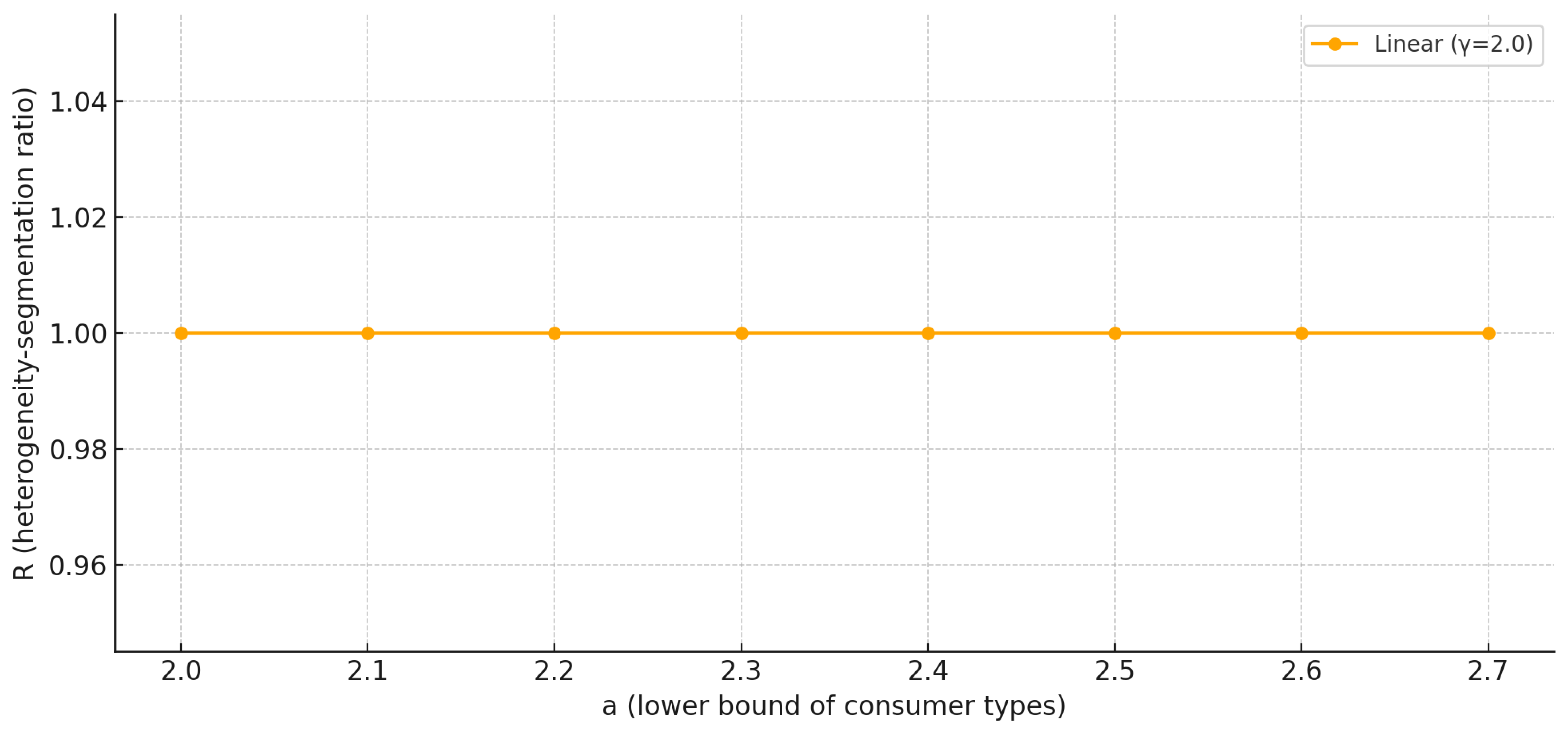
We extend the numerical analysis in

Table 1. Constant segmentation ratio $R=1$ under fully served equilibrium ($a\ge 2$).

a	$\mathit{b}=3$	$\underset{¯}{\mathbf{q}}=\mathit{a}/2$	$\overline{\mathit{q}}=3/2$	$\mathit{R}=\frac{\mathit{b}}{\mathit{a}}:\frac{\overline{\mathit{q}}}{\underset{¯}{\mathbf{q}}}$
2.0	3	1.00	3/2	1
2.1	3	1.05	3/2	1
2.2	3	1.10	3/2	1
2.3	3	1.15	3/2	1
2.4	3	1.20	3/2	1
2.5	3	1.25	3/2	1
2.6	3	1.30	3/2	1
2.7	3	1.35	3/2	1

to cover the case of a fully served equilibrium for all $a\ge 2$. In this regime, the marginal cost condition $C^{\prime }\left({\underset{¯}{q}}^W\right)=2$q${}^W=a$ implies that q $=a/2$. Substituting $b=3$, $\overline{q}=3/2$, and q $=a/2$ into the segmentation ratio R, we obtain

$$R={\displaystyle \frac{b}{a}}:{\displaystyle \frac{\overline{q}}{\underset{¯}{q}}}={\displaystyle \frac{3}{a}}:{\displaystyle \frac{3/2}{a/2}}=1.$$

This confirms that under linear marginal cost, the segmentation ratio remains constant as a increases within the fully served regime.

Figure 1 illustrates the case of a linear marginal cost function, where the segmentation ratio R remains constant across different values of a within the fully served equilibrium regime. This outcome aligns with the model’s prediction that $R=1$, reflecting a one-to-one correspondence between consumer heterogeneity and the range of product qualities offered.

Example 2 

(Strictly Convex Marginal Cost). Let $T=\left[a,20\right]$, $\overline{Q}=3$ and $C\left(Q\right)=Q^3$, implying that $C^{\prime }\left(Q\right)=3Q^2$, with $\gamma =3>2$.

The highest quality satisfies

$$C^{\prime }\left({\overline{q}}^W\right)=3{\left({\overline{q}}^W\right)}^2=20\Rightarrow {\overline{q}}^W=\sqrt{{\displaystyle \frac{20}{3}}}={\overline{q}}^E=\overline{q}.$$

We solve for the lowest quality under the partially served equilibrium:

$$20+{\left({\underset{¯}{q}}^2\right)}^E-6{\left({\underset{¯}{q}}^2\right)}^E=0\Rightarrow {\underset{¯}{q}}^E=2,$$

where q $=Max\{{\underset{¯}{q}}^E$,q${}^W\}=Max\{2$,q${}^W\}$.

• Subcase I. $a=12$:
• Since $b=20=2a-C\left({\underset{¯}{q}}^W\right)/$q${}^W=24-4=20$, the market is fully served. Here, $a=12$ is the critical value - -meaning that the market is fully served for all $a\ge 12$ and only partially served for all $0<a<12$.
• In this case, $C^{\prime }\left({\underset{¯}{q}}^W\right)=3($q${}^W)^2=12$⇒ q${}^W=2=$q${}^E=$q. We have

  $${\displaystyle \frac{b}{a}}={\displaystyle \frac{20}{12}}={\displaystyle \frac{5}{3}},{\displaystyle \frac{\overline{q}}{\underset{¯}{q}}}={\displaystyle \frac{\sqrt{20/3}}{2}}=\sqrt{{\displaystyle \frac{5}{3}}}\Rightarrow R={\displaystyle \frac{b}{a}}:{\displaystyle \frac{\overline{q}}{\underset{¯}{q}}}=\sqrt{{\displaystyle \frac{5}{3}}}>1.$$
• Subcase II. $a=15$:
• Since $b=20\le 2a-C\left({\underset{¯}{q}}^W\right)/$q${}^W=30-1.25=28.75$, the market is fully served.
• Here, $C^{\prime }\left({\underset{¯}{q}}^W\right)=3($q${}^W)^2=15$⇒ q${}^W=\sqrt{5}=\underset{¯}{q}>{\underset{¯}{q}}^E$. We have

  $${\displaystyle \frac{b}{a}}={\displaystyle \frac{20}{15}}={\displaystyle \frac{4}{3}},{\displaystyle \frac{\overline{q}}{\underset{¯}{q}}}={\displaystyle \frac{\sqrt{20/3}}{\sqrt{5}}}=\sqrt{{\displaystyle \frac{4}{3}}}\Rightarrow R={\displaystyle \frac{b}{a}}:{\displaystyle \frac{\overline{q}}{\underset{¯}{q}}}=\sqrt{{\displaystyle \frac{4}{3}}}>1.$$

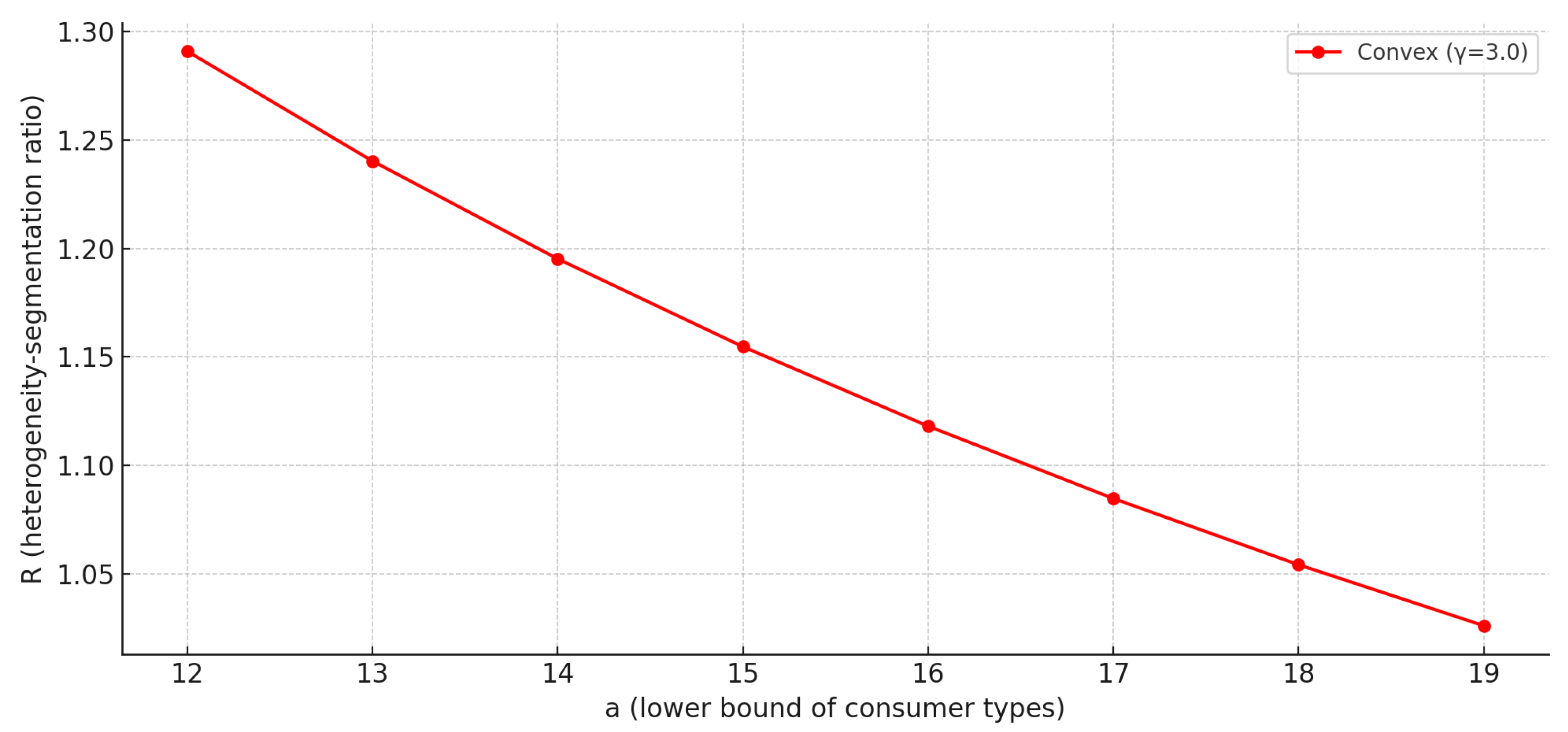
We extend the numerical analysis in

Table 2. Segmentation ratio $R=\sqrt{{\displaystyle \frac{20}{a}}}$ under fully served equilibrium ($a\ge 12$).

a	$\mathit{b}=20$	$\underset{¯}{\mathbf{q}}=\sqrt{\frac{\mathit{a}}{3}}$	$\overline{\mathit{q}}=\sqrt{\frac{20}{3}}$	$\mathit{R}=\frac{\mathit{b}}{\mathit{a}}:\frac{\overline{\mathit{q}}}{\underset{¯}{\mathbf{q}}}=\sqrt{\frac{20}{\mathit{a}}}$
12	20	2	$\sqrt{{\displaystyle \frac{20}{3}}}$	$\sqrt{{\displaystyle \frac{5}{3}}}$
13	20	$\sqrt{{\displaystyle \frac{13}{3}}}$	$\sqrt{{\displaystyle \frac{20}{3}}}$	$\sqrt{{\displaystyle \frac{20}{13}}}$
14	20	$\sqrt{{\displaystyle \frac{14}{3}}}$	$\sqrt{{\displaystyle \frac{20}{3}}}$	$\sqrt{{\displaystyle \frac{10}{7}}}$
15	20	$\sqrt{5}$	$\sqrt{{\displaystyle \frac{20}{3}}}$	$\sqrt{{\displaystyle \frac{4}{3}}}$
16	20	$\sqrt{{\displaystyle \frac{16}{3}}}$	$\sqrt{{\displaystyle \frac{20}{3}}}$	$\sqrt{{\displaystyle \frac{5}{4}}}$
17	20	$\sqrt{{\displaystyle \frac{17}{3}}}$	$\sqrt{{\displaystyle \frac{20}{3}}}$	$\sqrt{{\displaystyle \frac{20}{17}}}$
18	20	$\sqrt{6}$	$\sqrt{{\displaystyle \frac{20}{3}}}$	$\sqrt{{\displaystyle \frac{10}{9}}}$
19	20	$\sqrt{{\displaystyle \frac{19}{3}}}$	$\sqrt{{\displaystyle \frac{20}{3}}}$	$\sqrt{{\displaystyle \frac{20}{19}}}$

to cover the case of a fully served equilibrium for all $a\ge 12$. In this setting, the marginal cost condition $C^{\prime }\left({\underset{¯}{q}}^W\right)=3{\left({\underset{¯}{q}}^W\right)}^2=a$ implies that q $=\sqrt{{\displaystyle \frac{a}{3}}}$. Substituting $b=20$, $\overline{q}=\sqrt{{\displaystyle \frac{20}{3}}}$, and q $=\sqrt{{\displaystyle \frac{a}{3}}}$ into the segmentation ratio R, we obtain

$$R={\displaystyle \frac{b}{a}}:{\displaystyle \frac{\overline{q}}{\underset{¯}{q}}}={\displaystyle \frac{20}{a}}:{\displaystyle \frac{\sqrt{20/3}}{\sqrt{a/3}}}=\sqrt{{\displaystyle \frac{20}{a}}}.$$

This confirms that under a strictly convex marginal cost function, consumer heterogeneity grows faster than market segmentation - i.e., the segmentation ratio R is strictly greater than 1 and declines with a.

Figure 2 shows the behavior of R under a strictly convex marginal cost function. As the parameter a increases, the segmentation ratio $R=\sqrt{{\displaystyle \frac{20}{a}}}$ declines. This reflects the key result that consumer heterogeneity increases more rapidly than the range of qualities offered by the monopolist. In other words, convex marginal costs dampen the monopolist’s incentive to match rising heterogeneity with an equally broad quality spectrum.

Example 3 

(Strictly Concave Marginal Cost). Let $T=\left[a,4\right]$, $\overline{Q}=8$ and $C\left(Q\right)=Q^{3/2}$, implying that $C^{\prime }\left(Q\right)={\displaystyle \frac{3}{2}}{Q}^{1/2}$, with $\gamma =3/2<2$.

The highest quality satisfies

$$C^{\prime }\left({\overline{q}}^W\right)={\displaystyle \frac{3}{2}}{\left({\overline{q}}^W\right)}^{1/2}=4\Rightarrow {\overline{q}}^W={\displaystyle \frac{64}{9}}={\overline{q}}^E=\overline{q}.$$

We solve for the lowest quality under the partially served equilibrium:

$$4+{\left({\underset{¯}{q}}^{0.5}\right)}^E-3{\left({\underset{¯}{q}}^{0.5}\right)}^E=0\Rightarrow {\underset{¯}{q}}^E=4,$$

where q $=Max\{{\underset{¯}{q}}^E$,q${}^W\}=Max\{4$,q${}^W\}$.

• Subcase I. $a=3$:
• Since $b=4=2a-C\left({\underset{¯}{q}}^W\right)/$q${}^W=6-2=4$, the market is fully served. Here, $a=3$ is the critical value - -meaning that the market is fully served for all $a\ge 3$ and only partially served for all $0<a<3$.
• In this case, $C^{\prime }\left({\underset{¯}{q}}^W\right)={\displaystyle \frac{3}{2}}{\left({\overline{q}}^W\right)}^{1/2}=3$⇒ q${}^W=4=$q${}^E=$q. We have

  $${\displaystyle \frac{b}{a}}={\displaystyle \frac{4}{3}},{\displaystyle \frac{\overline{q}}{\underset{¯}{q}}}={\displaystyle \frac{64/9}{4}}={\displaystyle \frac{16}{9}}\Rightarrow R={\displaystyle \frac{b}{a}}:{\displaystyle \frac{\overline{q}}{\underset{¯}{q}}}={\displaystyle \frac{4/3}{16/9}}={\displaystyle \frac{3}{4}}<1.$$
• Subcase II. $a=3.75$:
• Since $b=4\le 2a-C\left({\underset{¯}{q}}^W\right)/$q${}^W=7.5-2=5.5$, the market is fully served.
• Here, $C^{\prime }\left({\underset{¯}{q}}^W\right)={\displaystyle \frac{3}{2}}{\left({\overline{q}}^W\right)}^{1/2}=3.75\Rightarrow$ q${}^W={\displaystyle \frac{25}{4}}=\underset{¯}{q}>{\underset{¯}{q}}^E$. We have

  $${\displaystyle \frac{b}{a}}={\displaystyle \frac{4}{3.75}}={\displaystyle \frac{16}{15}},{\displaystyle \frac{\overline{q}}{\underset{¯}{q}}}={\displaystyle \frac{64/9}{25/4}}={\displaystyle \frac{256}{225}}\Rightarrow R={\displaystyle \frac{b}{a}}:{\displaystyle \frac{\overline{q}}{\underset{¯}{q}}}={\displaystyle \frac{16/15}{256/225}}={\displaystyle \frac{15}{16}}<1.$$

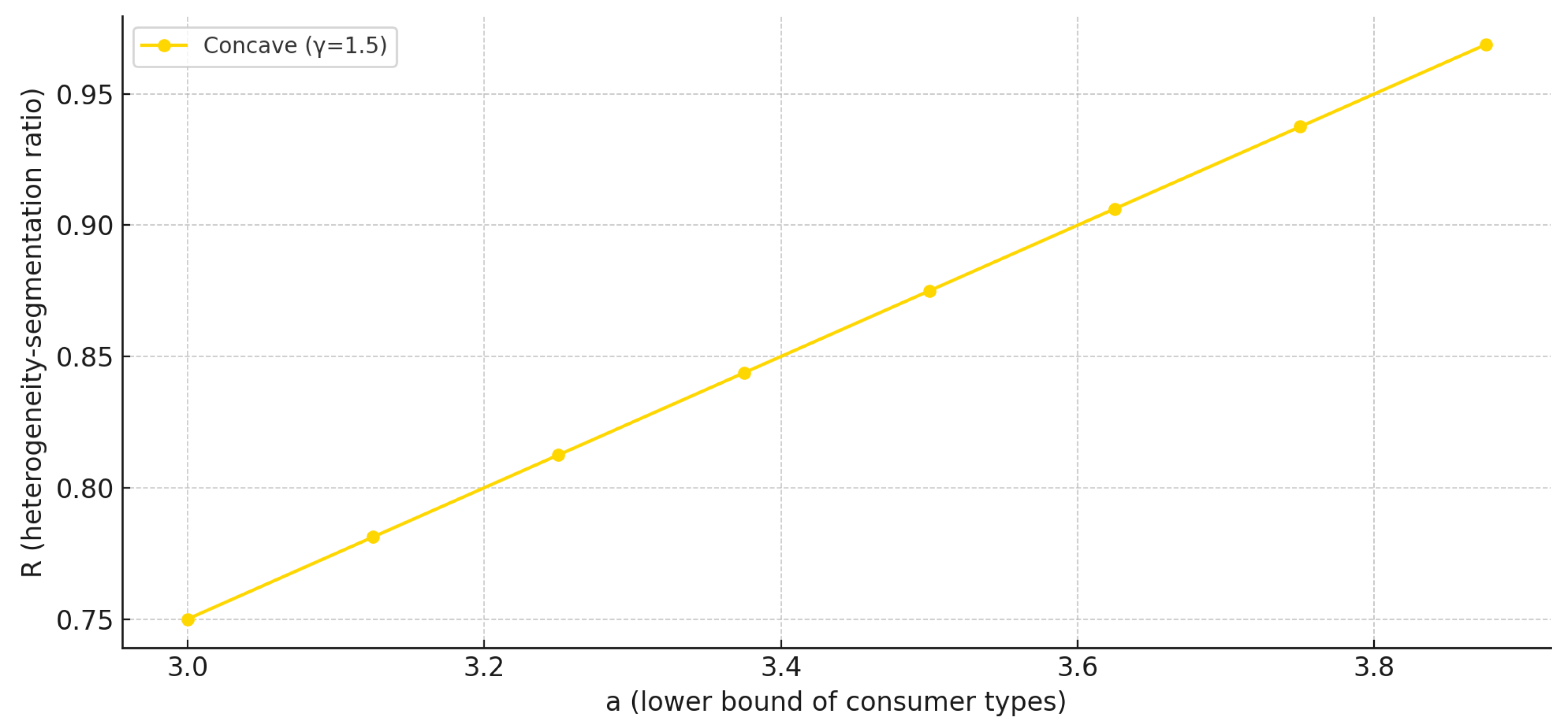
We extend the numerical analysis in

Table 3. Segmentation ratio $R={\displaystyle \frac{a}{4}}$ under fully served equilibrium ($a\ge 3$).

a	$\mathit{b}=4$	$\underset{¯}{\mathbf{q}}=\sqrt{\frac{\mathit{a}}{3}}$	$\overline{\mathit{q}}=\frac{64}{9}$	$\mathit{R}=\frac{\mathit{b}}{\mathit{a}}:\frac{\overline{\mathit{q}}}{\underset{¯}{\mathbf{q}}}=\frac{\mathit{a}}{4}$
3.000	4	2	${\displaystyle \frac{64}{9}}$	${\displaystyle \frac{3}{4}}$
3.125	4	$\sqrt{{\displaystyle \frac{13}{3}}}$	${\displaystyle \frac{64}{9}}$	${\displaystyle \frac{25}{32}}$
3.250	4	$\sqrt{{\displaystyle \frac{14}{3}}}$	${\displaystyle \frac{64}{9}}$	${\displaystyle \frac{13}{16}}$
3.375	4	$\sqrt{5}$	${\displaystyle \frac{64}{9}}$	${\displaystyle \frac{27}{32}}$
3.500	4	$\sqrt{{\displaystyle \frac{16}{3}}}$	${\displaystyle \frac{64}{9}}$	${\displaystyle \frac{7}{8}}$
3.625	4	$\sqrt{{\displaystyle \frac{17}{3}}}$	${\displaystyle \frac{64}{9}}$	${\displaystyle \frac{29}{32}}$
3.750	4	$\sqrt{6}$	${\displaystyle \frac{64}{9}}$	${\displaystyle \frac{15}{16}}$
3.875	4	$\sqrt{{\displaystyle \frac{19}{3}}}$	${\displaystyle \frac{64}{9}}$	${\displaystyle \frac{31}{32}}$

to cover the case of a fully served equilibrium for all $a\ge 3$. In this setting, the marginal cost condition $C^{\prime }\left({\underset{¯}{q}}^W\right)={\displaystyle \frac{3}{2}}{\left({\overline{q}}^W\right)}^{1/2}=a$ implies that q $={\left({\displaystyle \frac{2a}{3}}\right)}^2={\displaystyle \frac{4}{9}}{a}^2$. Substituting $b=4$, $\overline{q}={\displaystyle \frac{64}{9}}$, and q $={\displaystyle \frac{4}{9}}{a}^2$ into the segmentation ratio R, we obtain

$$R={\displaystyle \frac{b}{a}}:{\displaystyle \frac{\overline{q}}{\underset{¯}{q}}}={\displaystyle \frac{4}{a}}:{\displaystyle \frac{64/9}{(4/9)a^2}}={\displaystyle \frac{a}{4}}.$$

This confirms that under a strictly concave marginal cost function, market segmentation increases more rapidly than consumer heterogeneity - -i.e., the segmentation ratio R is strictly less than 1 and increases with a.

Figure 3 shows the segmentation ratio $R={\displaystyle \frac{a}{4}}$ for the case of a strictly concave marginal cost function. Here, R increases with a, confirming that market segmentation expands more rapidly than consumer heterogeneity. This result aligns with the model’s prediction that concave marginal costs amplify the monopolist’s responsiveness to increased heterogeneity by incentivizing a broader range of product qualities.

5. Discussion and Conclusions

This paper investigates a vertically differentiated monopoly model characterized by a strictly convex production cost function and a continuum of consumers under complete market segmentation. The central objective is to examine how the relationship between consumer heterogeneity and market segmentation is affected by the degree of convexity in the cost function.

The study makes three key contributions. First, it identifies the conditions under which there is equality between two ratios: the ratio of consumer heterogeneity, measured by $b/a$, and the ratio of quality differentiation, measured by $\overline{q}/$q. Second, it compares how changes in consumer heterogeneity influence market segmentation under different marginal cost structures - linear, strictly convex, and strictly concave. Third, it analyzes the divergence between fully and partially served equilibria in terms of their implications for consumer heterogeneity and market segmentation.

The main result reveals that, in a fully served market, the proportional relationship between consumer heterogeneity and market segmentation is governed by the convexity of the marginal cost function. This relationship is captured by the segmentation ratio $R={\displaystyle \frac{b/a}{\overline{q}/\underset{¯}{\mathrm{q}}}}$. Specifically, when the marginal cost $C^{\prime }\left(Q\right)$ is strictly convex, the segmentation ratio satisfies $R>1$, indicating that consumer heterogeneity increases more sharply than product differentiation (Example 2). When $C^{\prime }\left(Q\right)$ is strictly concave, $R<1$, meaning that market segmentation expands more rapidly than heterogeneity (Example 3). When $C^{\prime }\left(Q\right)$ is linear, $R=1$, reflecting a constant rate between heterogeneity and segmentation (Example 1, Parts I and II). In contrast, under a partially served equilibrium, this proportional relationship breaks down. Even with a linear cost function, changes in consumer heterogeneity do not lead to proportional adjustments in the quality range, causing the segmentation ratio R to vary and thus breaking the link between heterogeneity and market segmentation (Example 1, Parts II and III). This finding contrasts with Gabszewicz et al. (1986), whose framework excluded production costs and generated different segmentation dynamics.

Although welfare analysis is not the central focus of this paper, the findings have important policy implications. As shown in Gayer (2024), under similar conditions, a fully served equilibrium coincides with the welfare-maximizing allocation, whereas a partially served equilibrium represents a form of market failure, as some consumers who value the product do not purchase it. In this context, the present results suggest that cost curvature indirectly affects welfare by influencing whether full coverage is sustained and by shaping the balance between consumer heterogeneity and product variety. Policymakers concerned with welfare outcomes in vertically differentiated markets may therefore wish to consider how production cost structures - and the factors that drive them - affect both coverage and segmentation.

While the current analysis is theoretical, future research could explore potential empirical validation by examining data from industries where firms offer vertically differentiated products - such as automobiles, electronics, or education services - to test whether observed segmentation patterns align with the predicted effects of cost curvature. Furthermore, the framework could be extended to oligopoly settings, where strategic interaction between firms may alter the relationship between consumer heterogeneity and quality differentiation, potentially yielding richer market structures and different welfare outcomes.

References

1. Altan, B. (2020). Dynamic durable goods monopoly and market power. Games, 11(2), 22. [Google Scholar] [CrossRef]
2. Bagnoli, M., Salant, S. W., & Swierzbinski, J. E. (1989). Durable-goods monopoly with discrete demand. Journal of Political Economy, 97(6), 1459–1478. [Google Scholar] [CrossRef]
3. Besanko, D., Donnenfeld, S., & White, L. J. (1987). Monopoly and quality distortion: Effects and remedies. The Quarterly Journal of Economics, 102, 743–768. [Google Scholar] [CrossRef]
4. Bos, I., Cesi, B., & Marini, M. A. (2025). Cartel stability with quality-anchored buyers. Economics Letters, 254, 112449. [Google Scholar] [CrossRef]
5. Bos, I., & Marini, M. A. (2022). Collusion in quality-segmented markets. Journal of Public Economic Theory, 24(2), 293–323. [Google Scholar] [CrossRef]
6. Bos, I., Marini, M. A., & Saulle, R. D. (2020). Cartel formation with quality differentiation. Mathematical Social Sciences, 106, 36–50. [Google Scholar] [CrossRef]
7. Chander, P., & Leruth, L. (1989). The optimal product mix for a monopolist in the presence of congestion effects: A model and some results. International Journal of Industrial Organization, 7(4), 437–449. [Google Scholar] [CrossRef]
8. Dixit, A. K., & Stiglitz, J. E. (1977). Monopolistic competition and optimum product diversity. The American Economic Review, 67(3), 297–308. [Google Scholar]
9. Gabszewicz, J. J., Marini, M. A., & Tarola, O. (2016). Core existence in vertically differentiated markets. Economics Letters, 149, 28–32. [Google Scholar] [CrossRef]
10. Gabszewicz, J. J., Marini, M. A., & Tarola, O. (2017). Vertical differentiation and collusion: Pruning or proliferation? Research in Economics, 71(1), 129–139. [Google Scholar] [CrossRef]
11. Gabszewicz, J. J., Shaked, A., Sutton, J., & Thisse, J. F. (1986). Segmenting the market: The monopolist’s optimal product mix. Journal of Economic Theory, 39, 273–289. [Google Scholar] [CrossRef]
12. Gabszewicz, J. J., & Thisse, J. F. (1979). Price competition, quality and income disparities. Journal of Economic Theory, 20(3), 340–359. [Google Scholar] [CrossRef]
13. Gayer, A. (2007). Oligopoly, endogenous monopolist and product quality. The BE Journal of Theoretical Economics, 7(1), 1376. [Google Scholar] [CrossRef]
14. Gayer, A. (2014). Monopoly, social welfare, and multi product quality. Mathematical Economics Letters, 2(3–4), 51–57. [Google Scholar] [CrossRef]
15. Gayer, A. (2017). Endogenous duopolies. Economics Letters, 159, 1–3. [Google Scholar] [CrossRef]
16. Gayer, A. (2023). Duopoly and endogenous single product quality strategies. Games, 14(4), 56. [Google Scholar] [CrossRef]
17. Gayer, A. (2024). Monopoly and quality omission. Games, 15(6), 36. [Google Scholar] [CrossRef]
18. Motta, M. (1993). Endogenous quality choice: Price vs. quantity competition. The Journal of Industrial Economics, 41, 113–131. [Google Scholar] [CrossRef]
19. Mussa, M., & Rosen, S. (1978). Monopoly and product quality. Journal of Economic Theory, 18, 301–317. [Google Scholar] [CrossRef]
20. Noh, Y. H., & Moschini, G. (2006). Vertical product differentiation, entry-deterrence strategies, and entry qualities. Review of Industrial Organization, 29(3), 227–252. [Google Scholar] [CrossRef]
21. Phlips, L. (1983). The economics of price discrimination. Cambridge University Press. [Google Scholar]
22. Shaked, A., & Sutton, J. (1982). Relaxing price competition through product differentiation. The Review of Economic Studies, 49(1), 3–13. [Google Scholar] [CrossRef]
23. Shaked, A., & Sutton, J. (1983). Natural oligopolies. Econometrica: Journal of the Econometric Society, 51, 1469–1483. [Google Scholar]
24. Shitovitz, B., Spiegel, M., & Weber, S. (1989). ‘Top of the line’ quality as an optimal solution for a multi-quality monopolist. European Economic Review, 33, 1641–1652. [Google Scholar] [CrossRef]
25. Spence, M. (1976). Product selection, fixed costs, and monopolistic competition. The Review of Economic Studies, 43(2), 217–235. [Google Scholar] [CrossRef]
26. Spence, M. (1980). Multi-product quantity-dependent prices and profitability constraints. Review of Economic Studies, 47, 821–841. [Google Scholar] [CrossRef]
27. Yang, K. H. (2021). Efficient demands in a multi-product monopoly. Journal of Economic Theory, 197, 105330. [Google Scholar] [CrossRef]
Figure 1. Constant segmentation ratio R under linear marginal cost.
Games 16 00049 g001
Figure 2. Declining segmentation ratio R under convex marginal cost.
Games 16 00049 g002
Figure 3. Increasing segmentation ratio R under concave marginal cost.
Games 16 00049 g003