Abstract
This paper examines stochastic cooperation in markets with two sellers who exhibit one-sided dependency. The independent seller’s pricing influences the dependent seller’s demand, but not vice versa. We study the one-dimensional hybrid game class whose parameter is the exogenously given probability of cooperation. In each game of this class, both sellers simultaneously choose prices that determine their endogenous threats, i.e., conflict profits. The sellers are aware of the cooperation probability but cannot condition prices on whether or not there is cooperation. We characterize the equilibrium prices and the sellers’ expected profits. Our main result shows that the independent seller earns higher expected profits when cooperation is more likely. In contrast, the dependent seller earns lower expected profits when the likelihood of cooperation is below a threshold that we characterize explicitly, and higher profits are earned thereafter. These findings suggest that, within our framework, antitrust concerns may be mitigated. Since dependent sellers can incur losses from cooperation, collusion attempts become less viable in markets with one-sided dependency.
JEL Classification:
C72; C78; D43
1. Introduction
Economic analyses of markets with horizontally and vertically differentiated products have extensively examined collusion, cartel stability, and the effectiveness of antitrust interventions, emphasizing their dependence on factors such as product differentiation, cost asymmetries, and demand volatility (see Feuerstein, 2005; Marini, 2018, for surveys; see also Motta, 2004).1 These studies typically assume a two-sided dependency characterized by non-zero mutual cross-elasticities of demand (see, e.g., Varian, 1992, Chapter 16). In contrast, we focus on one-sided dependency, where the pricing of an independent seller affects the demand—and hence, the profit—of a dependent seller, while the reverse does not hold.
One-sided positive dependency occurs when a price reduction by the independent seller increases demand for the dependent seller’s product, while the reverse effect is negligible. This most likely occurs when the two goods are complementary in consumption. For example, in the market for printers and ink cartridges, a lower price of printers increases the demand for ink cartridges via increasing the demand for printers, yet a reduction in the price of ink cartridges would unlikely increase the demand for printers. Similarly, on markets for bicycles and helmets, lower prices of bicycles boost the demand for helmets, whereas the reverse effect is likely negligible.
In the case of one-sided negative dependence, a price cut by an independent seller reduces the demand of the dependent seller, whereas the same effect hardly works in the opposite direction. This asymmetry most likely occurs when the products are substitutes in consumption and are perceived by consumers as rather different in terms of quality or cultural characteristics. For instance, a price drop in luxury goods can reduce demand for cheaper alternatives, but the reverse is unlikely. Similarly, a reduction in the price of electric cars likely will negatively affect the demand for internal combustion engine vehicles, but the opposite is unlikely if the demand for electric vehicles is primarily driven by factors such as environmental concerns and fuel efficiency.
Due to the price externality, sellers may benefit from cooperating. For instance, they could form a cartel and share profits,2 or they could merge. Rather than examining specific cooperation arrangements, we analyze stochastic cooperation with joint profit maximization and equal surplus sharing for an exogenously given probability of cooperation. In our view, there are several reasons to assume that cooperation among (non-)mutually dependent sellers is stochastic. First, implementing collusive behavior requires sellers to coordinate multiple aspects of their interaction, the success of which is inherently uncertain. Second, collusion may evade detection by antitrust authorities, particularly when mistakenly perceived as random fluctuations in volatile markets.
Specifically, we analytically explore a one-dimensional hybrid game class, in which the parameter , with , is the exogenously given probability of cooperation. In each game of this class, both sellers choose prices simultaneously. As in Nash (1953), these prices determine their endogenous threats, i.e., the conflict profits defining the surplus from cooperation—given by the maximal joint profit minus the sum of the conflict profits.3 When setting prices, the sellers are aware of the cooperation probability, , but cannot condition prices on whether or not there is cooperation. Therefore, they only react to the commonly known cooperation probability. In line with Nash (1953), we assume that sellers commit to the prices chosen before the stochastic uncertainty is resolved.4
We characterize the equilibrium prices and expected profits from stochastic cooperation. Specifically, we examine whether each seller’s expected profit increases monotonically with the probability of cooperation, given a level of one-sided dependency. Our main result shows that the independent seller earns higher expected profits when cooperation is more likely. In contrast, the dependent seller earns lower expected profits when the likelihood of cooperation is below a threshold that we explicitly characterize, and profits are higher thereafter. In contrast, the dependent seller’s expected profits decrease with the probability of cooperation when this probability is below a threshold that we explicitly identify, and increase once the probability exceeds this threshold. Despite the inherent asymmetry, due to the one-sided externality, this result seems unexpected: one might have guessed that both sellers would benefit from cooperation, earning higher expected profits as cooperation becomes more likely.
Our results are related to two features of the model. First, when cooperation occurs, sellers prefer a larger share of the joint profit. This share increases with the difference between their own conflict profit and the other seller’s conflict profit. Second, the independent seller can leverage the price externality when balancing the change in their conflict profit with that in their share of the joint profit. Given these features, it follows from an envelope argument that the independent seller’s expected profit raises monotonically with the probability of cooperation. The same argument shows that, when cooperation is certain not to occur, raising the probability of cooperation has no first-order effect on the independent seller’s conflict profit, but it reduces the dependent seller’s conflict profit. This negative impact offsets the positive effect of a higher likelihood of surplus sharing on the dependent seller’s expected profits. However, we also demonstrate that these effects reverse when is large enough.
This paper is organized as follows: Section 2 introduces the model of stochastic cooperation; Section 3 derives and analyzes the best responses and the equilibrium prices; Section 4 derives the equilibrium expected payoffs and analyzes how they depend on the exogenous cooperation probability; Section 5 analyzes graphically the equilibrium quantities; Section 6 discusses some concluding remarks.
2. A Model of Stochastic Cooperation
Let denote the independent seller, to whom we also refer to as the “monopolist,” and denote the dependent seller. Furthermore, let denote the demand and the sale price of .
The (linear) demand functions are and . Here, captures the sign and strength of the price externality: the demand of D increases with when and decreases when .5 To avoid negative sales amounts, of course it will be ensured that and will hold. Moreover, to guarantee interior solutions to maximization problems below, we impose suitable restrictions on the parameters and , in addition to . Specifically, we present the following assumptions.6
Assumption 1.
and .
Furthermore, for the sets
we assume the following:
Assumption 2.
When , then must hold;
Assumption 3.
When , then must hold.
We neglect production costs so that the profits of the sellers are
When cooperating, sellers equally share the surplus from cooperation, i.e., the difference between their maximal joint profit and the sum of both profits in (1). When denotes the solution to
the surplus from cooperation is
The maximal joint profit is attained at the prices7
so that
It follows that holds trivially when , and it is due to Assumption 2 when .
According to the terminology of bargaining with variable threats (Nash, 1953), the profits in (1) define the threat point, i.e., they are the conflict profits in the case, while the agreement profits are
As mentioned in the Introduction, we analyze the class of hybrid games that arise when sellers cooperate with an exogenously given probability . In these games, the expected payoff of seller M is8
while the expected payoff of seller D is equal to
The second lines in (5) and (6) express the expected payoffs as the sum of the conflict profit and half of the cooperation surplus, being weighted by the probability of cooperation. The third lines show how payoffs depend on via a probability-weighted difference between each seller’s own conflict profit and that of the other.
3. Best Responses and Equilibrium Prices
The best responses and allow each seller to maximize their own expected payoff given the other seller’s price and are9
When , the best response of seller M is , which is independent of because of the one-sided dependency, and the associated profit is .10 When , the best response of seller M depends on the sign of : for positive (negative), seller M reduces (increases) its price relative to , with the adjustment becoming more pronounced when the likelihood of cooperation increases. This follows because seller M maximizes the expression , given . As a result, seller M has to balance the reduction in their own monopoly profit against the reduction in demand and profit of seller D via the price externality. Conversely, the best response of seller D does not depend on due to the one-sided dependency. This follows since D maximizes for a given , which is equivalent to maximizing , because does not depend on .
Furthermore, from (8), one derives the marginal effects of the change in on the equilibrium prices as12
Since ,13 decreases (increases) with when (). The intuition for this result is that a larger increases the weight of the negative component of D’s expected payoffs, , while it decreases the weight of the positive component, ; see Equation (5) above. Seller M optimally adjusts so that the reduction of compensates M in expectation for the reduction of , and the sign of the externality determines whether this lets marginally increase or decrease. Instead, is negative regardless of the sign of . The intuition for this is that, as increases, seller M adjusts , thus decreasing the demand of seller D, which in turn reduces .
4. Expected Equilibrium Payoffs
Let and denote the conflict equilibrium profits. Moreover, let denote the equilibrium surplus, which satisfies14
For seller , let denote the expected equilibrium payoff. Using the second expression in (5) and (6), direct computation yields
The total marginal effect of on is the sum of the direct effect when holding and —and thus the surplus—constant, and the indirect effect which accounts for the change in conflict profits and surplus due to changing and .
In order to characterize the indirect effects, one must take into account that profits vary with via equilibrium prices. However, according to a standard envelope argument, one might expect the first-order effects to vanish. In fact, and satisfy the following first-order conditions for interior solutions:
Therefore, when , the indirect effect (12) is equal to
since holds. From (12) and (15), one has
and, since holds, the expected payoff of seller M unambiguously increases with the cooperation probability, which also implies that , i.e., the expected payoff is higher when cooperation is certain than when conflict is certain.
When , the indirect effect in (12) is equal to
Using (14) once again, one has
and therefore,
So finally, (12) and (18) imply that
By evaluating the derivatives at the (interior) solution to the seller’s own profit maximization problem, one has that for seller M, the first-order effect of the change in equilibrium prices is null due to the asymmetric price externality: changing has no direct effect on , and expected payoff maximization implies that the first-order effects of own pricing are zero for both sellers.
For seller D, the situation is different: while the first-order effect of changing is zero, the first-order effect of changing is . Since the first term in (19) is positive and the second is negative when (see (11)), it may be that the expected payoff of seller D decreases as the cooperation probability rises. To get an intuition for this result, while both sellers prefer a larger share of the maximum joint profit in case of cooperation, they rather seek a larger conflict profit if they do not. Each seller’s share in the case of cooperation depends positively on the difference between their own conflict profit and that of the other seller (see the third line in (6)). Starting from , an increase in the probability of cooperation has no first-order effect on seller M’s conflict profit, while it has a negative first-order effect on seller D’s conflict profit (see (13) and (17)). The negative effect on seller D’s expected payoff, due to the smaller conflict profit, offsets the positive effect due to a larger likelihood of sharing the surplus from cooperation. However, from (19), one might suppose that these effects could reverse as rises, meaning that the expected payoff of seller D eventually increases with the likelihood of cooperation. The next proposition confirms this intuition by identifying the threshold cooperation probability, , below which decreases as rises, and above which it increases.
Proposition 1.
For a given α, the equilibrium payoff of seller D, , decreases with β when and increases when , where
Proof.
See Appendix C.2. □
Furthermore, for seller D, it also holds that the expected payoff is higher when cooperation is certain than when conflict is certain, i.e., one has15
Let us finally discuss two possible modifications to our model. One idea is to avoid the assumption that surplus is shared equally among firms. While this is rather natural and focal, one can also assume unequal surplus sharing.16 To this end, let be the surplus share of seller with , so that the agreement profits (4) are
and the expected profits (5) and (6) for the two sellers can be presented as:
and
for seller D. In this case, the equilibrium prices can be computed as in Appendix B, setting . Provided that , so that prices are interior, the qualitative features of our analysis will be preserved.
Another possible modification is to explicitly account for production costs.17 One approach is to assume that the marginal cost of production is constant and equal across sellers. In this case, the prices of sellers M and D would represent unit profit. With a suitable reinterpretation of the model’s parameters, the main qualitative results will remain unaffected.
5. A Graphical Analysis of the Equilibrium Quantities
In this section, we graphically simulate the equilibrium quantities as varies exogenously. To maintain consistency with the main analysis in the previous section, we assume equal surplus sharing. Moreover, to simplify the exposition and create noticeable visual effects, we also assume that and .
Figure 1, with in the left panel and in the right panel, plots agreement profits (dotted lines) and conflict profits (dashed lined) as varies between 0 and , and is set according to , as in (7). In all cases, the green lines pertain to seller M and the brown lines to seller D. The solid lines represent the equilibrium expected payoffs and as varies between 0 and 1. The three dots on these lines, moving leftward in the left panel and rightward in the right panel, correspond to and , respectively.
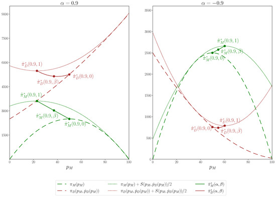
Figure 1.
Agreement profits, conflict profits, and equilibrium expected payoffs.
When , the expected payoffs coincide with the conflict profits, and the equilibrium values coincide with the non-cooperative ones. As increases, according to (9) and (10), seller M and D reduce their price when , and they increase it when . Furthermore, as shown in the figure, when , the first-order effect on seller M’s conflict profit is zero, while it is negative for seller D. As increases, the conflict profit curve of seller D, which is initially steeper than that of seller M, flattens, and the difference in the reduction of conflict profits shrinks. Initially, this allows seller M to increase its own equilibrium expected payoff at seller D’s expense. Subsequently, both sellers’ expected profits increase with the likelihood of cooperation.
Figure 2 shows an alternative representation of profits and expected payoffs when and .18 The dotted red line, referred to as , is the conflict profit frontier, i.e., the locus of conflict profit combinations. The continuous section of this line shows the conflict profit combinations as varies. Specifically, for a given , the point denoted by identifies the combination . The dotted blue line, referred to as , represents the combinations of profits that add up to , which can be achieved via side payments among the sellers. The continuous section of this line shows the combinations of agreement profits as varies. Specifically, for a given , the point denoted by identifies the combination . Finally, in clockwise order, the green dots and line represent the combinations of sellers’ expected payoffs for and 1, respectively, when . The difference in how the expected payoffs of sellers M and D vary with is also clearly apparent in this case.
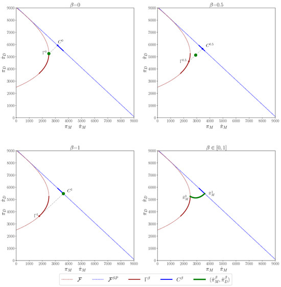
Figure 2.
Conflict and agreement profit frontiers and equilibrium expected payoffs ().
6. Conclusions
Our analysis of the one-dimensional hybrid game class, parameterized by the exogenous probability of cooperation, shows that the dependent seller’s expected payoff falls below the non-cooperative payoff when the probability of cooperation is low enough. However, when the probability of cooperation is greater than a critical threshold, the dependent seller’s expected payoff exceeds the non-cooperative payoff and rises with the probability of cooperation. This non-monotonicity of the expected payoff highlights an asymmetry which could provide some insights for more extended analyses aiming at investigating the factors which determine the likelihood of cooperation. For example, while a low probability of cooperation may stem from volatile market conditions, it may also stem from dependent sellers boycotting the attempt to establish any system of coordination among sellers. Moreover, in case communication is necessary to support collusion (as for instance in Aubert et al., 2006), the dependent firm can whistle-blow any attempt to promote cartelization by the monopolist.19 Furthermore, substantially increasing the probability of cooperation more likely attracts scrutiny, provokes public discussion, and potentially leads to prosecution. In practice, the probability of cooperation—assumed here to be exogenously given—is likely shaped by efforts to establish, maintain, and, if necessary, conceal cooperative arrangements. Successful cooperation may even require sellers to disclose private information, creating an additional barrier to its initiation and reinforcement.
In such cases, the incentive to engage in cooperative behavior is weak, possibly deterring the dependent seller from participating in collusion attempts. A final implication of our analysis is that, within our framework, antitrust concerns may be attenuated. Since dependent sellers can incur losses from cooperation, such arrangements become less viable. When unanimity among sellers is required for cooperation, the non-monotonic incentives faced by dependent sellers further reduce the likelihood of collusive agreements in cases of one-sided dependencies between sellers.
Finally, we suggest two directions for future research: First, the analysis could be extended to consider the possibility that the cooperation probability is endogenously determined.20 Second, the theoretical analysis could be complemented with an experimental analysis that investigates the behavioral implications of our model.
Author Contributions
Conceptualization, L.F., W.G., V.L. and L.P.; Methodology, L.F., W.G., V.L. and L.P.; Formal analysis, L.F., W.G., V.L. and L.P.; Writing—original draft, L.F., W.G., V.L. and L.P.; Writing—review & editing, L.F., W.G., V.L. and L.P. All authors have read and agreed to the published version of the manuscript.
Funding
Luca Panaccione acknowledges the support of the Italian Ministry of University and Research (PRIN 20229LRAHK).
Data Availability Statement
The original contributions presented in the study are included in the article, further inquiries can be directed to the corresponding author.
Acknowledgments
We thank the referees for their useful comments. Lorenzo Ferrari acknowledges that the views and opinions expressed in this article are strictly those of the author and they do not reflect in any way those of the Institution to which he is affiliated.
Conflicts of Interest
The authors declare no conflicts of interest.
Appendix A. Related to Section 2
Appendix A.1. Assumptions
Recall that we assume , and we define
Moreover, recall that Assumptions 1–3 introduced in Section 2 regarding and require that:
- (1)
- and ;
- (2)
- if , and ;
- (3)
- if , .
Figure A1 and Figure A2 represent the sets and , respectively, when Assumption 1 holds. The shaded area illustrates the pairs which satisfy Assumption 2 and Assumption 3.

Figure A1.
.

Figure A2.
.
The above assumptions imply some conditions which will be used in what follows. Therefore, for the sake of clarity, we list them here so that can be recalled when necessary.
When and , one has , and therefore, . It follows that, in this case, Assumption 3 implies that . When , Assumption 1 implies that whenever . Altogether, if , Assumptions 1 and 3 imply that
When , one has , and therefore, . It follows that, in this case, Assumption 3 implies that . When , Assumption 1 implies that . By the same reasoning, one has holds for both and . Altogether, Assumptions 1 and 3 imply that
Appendix A.2. Derivation of Equations (2) and (3)
To maximize the joint profits , one solves the following problem:21
Recall that and . Let and be the multipliers associated with the first and second constraint, respectively. The Kuhn–Tucker conditions are
Since is a strictly concave function of , because its Hessian matrix is negative-definite,22 conditions (A4)–(A7) are sufficient. To investigate all possible cases,23 we consider three scenarios:
- (i)
- and ,
- (ii)
- and ,
- (iii)
- and .
In scenario (i), (A6) and (A7) imply that and , respectively. Therefore, scenario (i) includes four cases:
- (i.a)
- (i.b)
- (i.c)
- (i.d)
In scenario (ii), (A6) implies that . Therefore, this scenario includes three cases:
- (ii.a)
- (ii.b)
- (ii.c)
Recall that, in scenario (iii), and hold, so this means that (A6) implies and (A7), which implies that . This scenario, therefore, includes two cases:
- (iii.a)
- and , which implies that, via (A5), ; hence, . However, by the usual argument, this is not possible.
- (iii.b)
- and , which implies that via (A5). However, this is not possible, since and imply that .
Summing up, the only admissible case is (i.d), which corresponds to interior values of both prices and , as given by (A8).
Appendix B. Related to Section 3
Appendix B.1. Derivation of Equation (7)
- First, we characterize the best response of seller M. Given , the seller M chooses to maximize the expected profits as
- (i)
- (ii)
- . In this case, (A17) implies that , and (A16) implies that ; hence, When , the condition is always satisfied, while the condition is verified provided that holds. When , the condition is always satisfied, while the condition is verified provided that holds. Summing up, we have that this case arises when .
- (iii)
- Summing up, the price which maximizes the expected profits of seller M is given by
- (i)
- (ii)
- (iii)
- Summing up, the only admissible case is , and therefore, the best response of seller D is
Appendix B.2. Derivation of Equation (8)
Before computing the equilibrium prices, we verify that one has if Assumptions 1–3 hold so that the equilibrium price of seller M will be interior. To this end, we verify that holds so that the result follows from (A18).
From (A21) and , one has . Therefore, it is enough to show that, if Assumptions 1–3 hold, one has , which is equivalent to
When , (A22) is equivalent to . Since and , one has . For the same reason, one also has , hence , and therefore, . It follows that one has , in which the second inequality holds because of Assumption 3.
When , (A22) is equivalent to . Since and , one has . Furthermore, since , one has , and therefore, . It follows that one has , in which the second inequality holds because of Assumption 2.
It follows that to compute the equilibrium prices, one can use (A21) and the first condition in (A18). Proceeding by substitiution, for the price of seller M, one has
which implies that
and hence,
Therefore, it follows that the price of seller D is given by
In what follows, we let and denote the equilibrium prices of seller M and D, respectively. Therefore, one has
Appendix B.3. Derivation of Equations (9) and (10)
As for Equations (9), one has
As for Equation (10), one has
Due to Assumption 1 the following holds . Hence, it follows that increases (decreases) with when (), whereas is decreasing with regardless of the sign of .
Appendix C. Related to Section 4
Appendix C.1. Derivation of Equation (11)
Let and . Firstly, we compute and . As for , one has
As for , it follows that
Hence, one has
Given and , the surplus is computed as follows:
It is straightforward to verify that the above expression is positive. Finally, from (A23), one has
which is always positive.
Appendix C.2. Derivation of Proposition 1
Using the results from Appendix C.1, one has
which is positive only if the term in the last round brackets is positive. The derivative is positive (negative) if the numerator of the term in square brackets is positive (negative). By focusing on this term, one has
Appendix C.3. Derivation of Equation (21)
The equilibrium expected payoff for is equal to
The non-cooperative profit of D is equal to
By comparing these values, one gets
Given the result above, and the fact that is continuous in and is first decreasing and then increasing in , we can conclude that there exists such that
Appendix D. Related to Section 5
Appendix D.1. The Profit Frontier When α < 0
Figure A3 replicates Figure 2 for when . Since the elements are the same, we refer the reader to the comment of Figure 2 for the explanation.

Figure A3.
Conflict and agreement profit frontiers and equilibrium expected payoffs ().
Notes
| 1 | While initial studies focused on horizontal and vertical cooperation separately, more recent papers have extended the analysis to settings involving both types of cooperation. See for instance Symeonidis (1999) and Sen et al. (2024). |
| 2 | See, e.g., Bolle and Güth (1992), who analyze theoretically mutual shareholding and assess it empirically for the German energy market. |
| 3 | The Nash (1953) model with variable threats (see also van Damme, 1991, Chapter 7.8) has been generalized for more than two players by Kaneko and Mao (1996), who also analyze the case with no commitment. Bolt and Houba (1998) instead consider an explicit dynamic bargaining stage. |
| 4 | If this assumption is removed, the analysis and its conclusions should be adapted accordingly. |
| 5 | When , both sellers would be independent monopolists. |
| 6 | See Appendix A.1 for a visualization of Assumptions 2 and 3 and some useful implications of Assumptions 1–3. |
| 7 | See Appendix A.2 for derivations. |
| 8 | We use “profits” when we refer to conflict or agreement and “expected payoffs” otherwise. |
| 9 | In Appendix B.1 it is shown that or are admissible best response with corner values. However, they are disregarded, since these values cannot arise in equilibrium when given our assumptions. |
| 10 | These values are the same as those resulting from a standard monopoly profit maximization problem. |
| 11 | See Appendix B.2 for derivations. |
| 12 | See Appendix B.3 for derivations. |
| 13 | When this follows from Assumption 2. |
| 14 | See Appendix C.1 for derivations. |
| 15 | See Appendix C.3 for derivations. |
| 16 | We thank one referee for suggesting that we also consider this case. |
| 17 | We thank one referee for this suggestion. |
| 18 | For completeness, Figure A3 in Appendix D illustrates the case . |
| 19 | In this respect, our results are in line with empirical findings of, among others, Besley et al. (2021) and Block et al. (1981). |
| 20 | We thank a referee for suggesting this extension. |
| 21 | The rather natural constraints are consistent with those associated to the non-cooperative profit maximization problem and guarantee that a solution exists for any parameter constellation. |
| 22 | Let and denote the second derivative of with respect to and , respectively. Then one has and due to (see, e.g., Mas-Colell et al., 1995, p. 937). |
| 23 | The variables and can assume either an interior value or one boundary value (out of two). Therefore, there are cases altogether. |
| 24 | In this problem, must also satisfy the constraint for a given . However, since the values of , which are ultimately admissible, maximize the expected payoff of seller D, this constraint is always satisfied. |
| 25 | Since we are ultimately interested in the equilibrium analysis, this restriction is without loss of generality. |
References
- Aubert, C., Rey, P., & Kovacic, W. E. (2006). The impact of leniency and whistle-blowing programs on cartels. International Journal of Industrial Organization, 24(6), 1241–1266. [Google Scholar] [CrossRef]
- Besley, T., Fontana, N., & Limodio, N. (2021). Antitrust policies and profitability in nontradable sectors. American Economic Review: Insights, 3(2), 251–265. [Google Scholar] [CrossRef]
- Block, M. K., Nold, F. C., & Sidak, J. G. (1981). The deterrent effect of antitrust enforcement. Journal of Political Economy, 89(3), 429–445. [Google Scholar] [CrossRef]
- Bolle, F., & Güth, W. (1992). Competition among mutually dependent sellers. Journal of Institutional and Theoretical Economics (JITE)/Zeitschrift für die gesamte Staatswissenschaft, 148(2), 209–239. [Google Scholar]
- Bolt, W., & Houba, H. (1998). Strategic bargaining in the variable threat game. Economic Theory, 11, 57–77. [Google Scholar] [CrossRef]
- Feuerstein, S. (2005). Collusion in industrial economics—A survey. Journal of Industry, Competition and Trade, 5, 163–198. [Google Scholar] [CrossRef]
- Kaneko, M., & Mao, W. (1996). N-person Nash bargaining with variable threats. The Japanese Economic Review, 47(3), 235–250. [Google Scholar] [CrossRef]
- Marini, M. A. (2018). Collusive agreements in vertically differentiated markets. In L. C. Corchón, & M. A. Marini (Eds.), Handbook of game theory and industrial organization volume II (pp. 34–56). Edward Elgar Publishing. [Google Scholar]
- Mas-Colell, A., Whinston, M. D., & Green, J. R. (1995). Microeconomic theory. Oxford University Press. [Google Scholar]
- Motta, M. (2004). Competition policy: Theory and practice. Cambridge University Press. [Google Scholar]
- Nash, J. F. (1953). Two-Person cooperative games. Econometrica, 21(1), 128–140. [Google Scholar] [CrossRef]
- Sen, N., Tandon, U., & Biswas, R. (2024). Collusion under product differentiation. Journal of Economics, 142, 1–43. [Google Scholar] [CrossRef]
- Symeonidis, G. (1999). Cartel stability in advertising-intensive and R&D-intensive industries. Economics Letters, 62(1), 121–129. [Google Scholar]
- van Damme, E. (1991). Stability and perfection of nash equilibria (Vol. 339). Springer. [Google Scholar]
- Varian, H. R. (1992). Microeconomic analysis. W.W. Norton & Company. [Google Scholar]
Disclaimer/Publisher’s Note: The statements, opinions and data contained in all publications are solely those of the individual author(s) and contributor(s) and not of MDPI and/or the editor(s). MDPI and/or the editor(s) disclaim responsibility for any injury to people or property resulting from any ideas, methods, instructions or products referred to in the content. |
© 2025 by the authors. Licensee MDPI, Basel, Switzerland. This article is an open access article distributed under the terms and conditions of the Creative Commons Attribution (CC BY) license (https://creativecommons.org/licenses/by/4.0/).