Abstract
In this work, we study n-agent Bayesian games with m-dimensional vector types and linear payoffs, also called linear multidimensional Bayesian games. This class of games is equivalent with n-agent, m-game uniform multigames. We distinguish between games that have a discrete type space and those with a continuous type space. More specifically, we are interested in the existence of pure Bayesian Nash equilibriums for such games and efficient algorithms to find them. For continuous priors, we suggest a methodology to perform Nash equilibrium searches in simple cases. For discrete priors, we present algorithms that can handle two-action and two-player games efficiently. We introduce the core concept of threshold strategy and, under some mild conditions, we show that these games have at least one pure Bayesian Nash equilibrium. We illustrate our results with several examples like the double-game prisoner’s dilemma (DGPD), the game of chicken, and the sustainable adoption decision problem (SADP).
1. Introduction
Game theory provides an abstract framework to model a broad range of decision-making scenarios in real-life situations. From social cooperation (Larson, 2021) to biological evolution (Friedman, 1998) and economics (Shapiro, 1989) we can find models of games that can help to predict, or at least explain, the decision-makers’ behavior. “Game theory is a bag of analytical tools designed to help us understand the phenomena that we observe when decision-makers interact” (Osborne & Rubinstein, 1994). A game is designed to model any situation involving decision-makers (players and/or agents) that are rational and reason strategically. An agent is rational when it has a well-defined objective, is able to identify a preferable situation, and attempts to maximize its payoff. Strategic reasoning is the use of knowledge in a manner that best anticipates the other agents’ actions and taking them into account in the decision process. The knowledge of an agent is the information that it has before making its decision. Information only known by one player is said to be private knowledge. When it is shared among a group of players, we say that this is common knowledge.
More formally, we assume that agents are indexed by a set I. We denote the set of actions of agents by A, the set of outcomes by O, and consider an outcome function that gives the outcome of a set of actions. The preferences of any agent are specified by the maximization of a utility (or payoff) function . The simplest form of a game is the Strategic Game given in Definition 1. An action profile is an outcome of the game. We use the index to designate “all players except i” and write for .
Definition 1.
A Strategic Game comprises the following:
- 1.
- A finite set of n agents.
- 2.
- For each agent , there exists a nonempty set of possible actions. If is finite for all agents, then we say that the game is finite.
- 3.
- A set of possible outcomes.
- 4.
- A set of utility functions specifying the preferences of agent i.
A Nash equilibrium (NE) “captures a steady state” (Osborne & Rubinstein, 1994) of a game in which all agents have no incentive to deviate from their action unilaterally (Definition 2).
Definition 2.
A Nash equilibrium of the strategic game is an action profile such that
For a set X, let denote its set of subsets.
Definition 3.
Given an agent i and the action , the best-response function is such that
This implies that is a Nash equilibrium if and only if .
The prisoner’s dilemma (PD) (Flood, 1958) is a widely used toy example that models a simple situation of self-interest driven decision and illustrates a case where the Nash equilibrium is not Pareto efficient (Osborne & Rubinstein, 1994). When extended to more than two agents, it is often associated with the tragedy of the commons (Carrozzo Magli et al., 2021). This is a situation in which “individuals, who have open access to a shared resource act independently according to their own self-interest and, contrary to the common good of all users, cause depletion of the resource through their uncoordinated action (Hardin, 1968).”
However, empirical evidence challenges this theoretical prediction. In (Poundstone, 1993), the authors observed that New Zealand’s unlocked newspaper boxes (where taking without paying is easy) function successfully. Rather than exploiting this vulnerability, most customers voluntarily pay, suggesting they understand that collective defection would collapse the system.
Consider, for example, the TV show “Friend or Foe?”, which aired between 2002 and 2005 in the US. Two players who previously failed to answer some questions have to play “The Trust Box”: if they both choose Friend, they share a specified amount of money. If they both choose Foe, the money is lost. If one plays Friend while the other plays Foe, the player choosing Foe wins all the money. Although (Friend, Friend) is not a NE, data collected from this kind of game showed that in such situation, “cooperation is surprisingly high” (van den Assem et al., 2011). Experience suggests that when a significant amount of money is at stake, players tend to cooperate. Indeed, humans are not only driven by material considerations but also by moral and sociocultural matters.
1.1. Bayesian Games
Concrete situations usually involve uncertainty at multiple levels so Strategic Games with perfect information (such as the prisoner’s dilemma or hawk–dove (Székely et al., 2010)) may not be sufficient to describe the game. Usually, we denote this unknown information as a state of nature and model it with a state space (Osborne & Rubinstein, 1994). Suppose each agent has some private information (or private knowledge): this information, called the type of agent i, is unknown to the other agents, who can only have a (subjective) probability distribution over such possible types for an agent. So, we assume that they have in mind a type space and a probability measure over , and, following von Neumann and Morgenstern’s theory (von Neumann & Morgenstern, 1944), they play that maximizes the expected value of subject to .
A game G is Bayesian (Harsanyi, 1967, 1968a, 1968b) when there is uncertainty for the agents (as in Definition 4). In this situation, an agent can no longer anticipate the output of the game with certainty because some information about the game is unknown. Variance in the outcome is generally associated with risk or “how much we could diverge from what we expect”. A human player who wants to maximize his/her payoff without taking too much risk could be modeled by optimizing a combination of the expected value and the associated variance, as seen in portfolio management models (Luenberger, 1998).
A key feature of Bayesian games is that strategies are functions of agents’ types, mapping from private information to action choices. Indeed, the action of an agent depends on all the information it has (its own type) at the moment of the decision. We distinguish pure strategies from mixed strategies , where denotes the set of all probability distributions on a set X. In the latter case, the action played is no longer deterministic but chosen randomly according to a probability distribution.
Definition 4.
A Bayesian game G is a game in strategic form with incomplete information which we denote by where
- 1.
- is the set of agents.
- 2.
- is agent i’s action set and is the set of action outcomes or action profiles.
- 3.
- is agent i’s type space and is the set of type profiles.
- 4.
- is agent i’s utility for each .
- 5.
- is a (subjective) joint probability on Θ for each .
For such games, we can derive the notion of Bayesian Nash equilibrium from the NE of strategic games where we maximize an expected utility subject to agents’ types. We also distinguish pure and mixed Nash equilibria. Thanks to the Nash theorem (Theorem 1), we know that there always exists a mixed-strategy Nash equilibrium (denoted by mixed NE). However, this theorem does not give a practical method to find this Nash equilibrium. In fact, finding a Nash equilibrium is often very complex and cannot be computed in a reasonable time. In 1994, Christos H. Papadimitriou introduced the complexity class PPAD (polynomial parity arguments on directed graphs) (Papadimitriou, 1994) in order to classify the problem of finding a Nash equilibrium. Later, he also showed that the problem of finding a Nash equilibrium for a finite game is PPAD-complete (Daskalakis et al., 2009).
Theorem 1
(Nash Theorem (Osborne & Rubinstein, 1994)). Every finite strategic game has a mixed-strategy Nash equilibrium.
Although finding a Nash equilibrium is very hard in general, we can find some classes of games that have nice properties and an efficiently computable Nash equilibrium (Rabinovich et al., 2013).
1.2. Linear Multidimensional Bayesian Games
For our study, we consider linear multidimensional Bayesian games (Definition 5). They were initially introduced by Krishna and Perry to model multiple object auctions (Krishna & Perry, 1998). This class of games was shown (Edalat et al., 2018) to be equivalent to another class of games called uniform multigames (Theorem 2). A multigame (Definition 6) is a game that comprises several local games that are played simultaneously by all agents. Each local game has its own payoff matrix and possible actions. For example, an agent playing “Head or Tail” with one person and “Rock, Paper, Scissors” with another person simultaneously can be modeled by a multigame. Even if both local games are solved simultaneously, the agent is just playing on two “separate” games and tries to maximize a global utility which is a linear combination of local utilities. More specifically, for multigames in which every agent has the same set of actions in all local games, we can consider uniform games: agents can only take the same action in all local games. When a multigame is uniform, an agent chooses only one strategy that is played identically in all local games. In other words, one decision has multiple consequences and each agent wants to optimize their overall utility. An agent chooses a global strategy that is applied to all the local games. Let denote the set of non-negative real numbers.
Definition 5 (Linear Multidimensional Bayesian Games).
A Bayesian game G is m-dimensional if the type space of each agent is a bounded subset of . When the positive integer is implicitly given, we say that G is multidimensional. A multidimensional Bayesian game is linear if the utility of each agent only depends linearly on its own type components, i.e., there exists such that .
Definition 6.
A multigame
is a game in strategic form with incomplete information with the following structure:
- 1.
- The set of agents .
- 2.
- The set of n-agent basic games is given by , where with action space and utility function for each agent in the game .
- 3.
- Agent i’s strategy is where is agent i’s action in .
- 4.
- Agent i’s type is with , and .
- 5.
- Agent i’s utility for the strategy profile and type profile depends linearly on its types:
- 6.
- The agents’ type profile is drawn from a given joint probability distribution . For any , the function specifies a conditional probability distribution representing what agent i believes about the types of the other agents if its own type where .
The type coefficients represent agent i’s weight or priority for game j, reflecting how much agent i values outcomes in that particular game relative to others.
Theorem 2
(Edalat et al., 2018). Suppose that G is a linear m-dimensional Bayesian game with a bounded type space for each ; then, G is equivalent with a uniform multigame with m basic games.
Note that according to Definition 6, the type can be any m-dimensional vector with positive coefficients. We say that a multigame is normalized when . Any multigame can be converted into a normalized multigame by adding a well-chosen local game (Edalat et al., 2018). Thus, we can assume without loss of generality that multigames are normalized; as such, all agents’ type coefficients add up to 1. As previously mentioned, this paper focuses on uniform multigames that have the following two basic features: (1) identical action sets in all local games for every agent , i.e., and (2) each agent plays the same action in all basic games , i.e., . Additionally, we assume that the agents’ types are independent
We aim to show, beyond what is provided in (Edalat et al., 2018), that the multigame framework can model a wide range of complex situations that are worth exploring such as coordinated international environmental and social actions. First, consider a situation in which two countries could either keep an unsustainable traditional production system or shift to more responsible production. This shift is only beneficial if both countries commit to it. However, each country can be tempted to keep the old traditional production system, which does not incur an additional cost and is more efficient and profitable (at least this is what agents trust). This situation falls into the original prisoner’s dilemma framework, and we end up with a situation where both countries keep their traditional production (assuming that they act rationally).
Now, we extend this situation to N companies in the same geographical area. We assume that each company that continues to keep an unsustainable production unit causes a pollution cost of 1 unit. Thus, the (shared) pollution cost k is the number of companies that do not shift their production unit, . On the other hand, a company that shifts its production unit for a more sustainable one has to pay an additional (fixed) cost . Thus, represents a company i that shifts its production and is a company that keeps it. If all N agents shift, they all end up with a (small) cost c, and if no agent does so, they all end up with a (high) cost of N. Therefore, it is in the common interest that everyone shifts their production unit. However, as each individual company has no incentive to deviate from not shifting, the only Nash equilibrium of this game occurs when they all avoid the shift. The latter example can handle any number of companies but remains very limited as we cannot include the particularities of the agents (types) and the uncertainty about what other companies value the most (i.e., the Bayesian aspect).
Later on, we study a more powerful approach through the multigames framework. We call it the Sustainable Adoption Decision Problem (SADP): n independent countries share m possible concerns like population well-being, air pollution, economic stability, education, or preserving biodiversity. Each country has its own (subjective) priorities characterized by an m-dimensional vector and has to choose between keeping their current lifestyle or radically shifting to a more sustainable one.
We denote using a uniform multigame with n agents, m local games, and a number of possible actions, assuming that all agents have the same number of possible actions. When we have games with two actions (), we call these two actions C (cooperation) and D (defection). In this paper, we study multigames with continuous type space and show that with a simple condition on local games, the existence of a pure Bayesian Nash equilibrium is guaranteed. At the same time, we define the notion of threshold strategy and discuss the possibility to extend it to any number of actions. Then, we operate the same kind of analysis for discrete games. For both continuous and discrete type spaces we define a particular kind of multigame that is called double-game prisoner’s dilemma (DGPD). In the final part, we propose algorithms that can efficiently find NE in particular situations and formulate postulates by exploring some properties of multigames.
1.3. Motivations and Applications
Real-world decision-makers rarely optimize a single objective. Firms balance profit against environmental impact and reputation (Porter & Kramer, 2011), countries weigh economic growth against sustainability (Stern, 2007), and investors consider returns alongside risk and social responsibility (Friede et al., 2015). These multidimensional preferences, combined with incomplete information about others’ priorities, motivate our study of linear multidimensional Bayesian games.
Our focus on pure (Nash) equilibria reflects their practical relevance. When organizations like companies or government decide whether to adopt sustainable practices or negotiate agreements, decisions are typically binary rather than probabilistic mixtures (Heal & Kunreuther, 2011). Pure strategies offer clearer interpretation and direct implementation. The threshold strategies we identify—where agents act based on whether their type exceeds a critical value—naturally capture many real-world decision rules and provide tractable equilibrium characterizations.
The computational algorithms we develop bridge theory and practice. While equilibrium existence is guaranteed theoretically, finding equilibria in multidimensional games remains computationally challenging (Rabinovich et al., 2013). Our algorithms exploit the linear payoff structure to achieve efficiency, enabling analysis of realistic scenarios.
Applications span multiple domains. In environmental economics, our Sustainable Adoption Decision Problem (SADP) captures how countries with heterogeneous priorities over economic and environmental objectives can reach stable agreements without central coordination (Nordhaus, 2015). In corporate strategy, firms competing while balancing profit, social responsibility, and reputation can achieve stable market configurations when each has private information about its own priorities. Financial markets exhibit similar dynamics as investors with diverse preferences over return, risk, and ESG criteria reach equilibrium allocations (Pástor et al., 2021).
This framework addresses pressing global challenges requiring multidimensional trade-offs under uncertainty—climate change mitigation, pandemic response, sustainable development. By proving that pure equilibria exist in broad game classes and providing efficient algorithms to find them, we offer both theoretical insights and practical tools for policy design. The threshold structure reveals how incremental changes in preferences can trigger discrete behavioral shifts (Granovetter, 1978), while our classification of games illuminates which structures guarantee stable outcomes. These contributions suggest natural extensions to games with more actions and correlated types, suggesting promising directions for future research.
1.4. Related Work
While (Krishna & Perry, 1998) introduced linear multidimensional Bayesian games for multi-object auctions, the literature on multidimensional games extends significantly beyond this foundation. (Reny, 2011) studied monotone equilibria in multi-unit auctions with interdependent values, and (Athey, 2001) characterized monotone equilibria in games with single-dimensional types, providing techniques partially applicable to multidimensional settings. The complexity of multidimensional mechanism design has been explored by (Manelli & Vincent, 2007), who analyzed revenue maximization in multiple-good monopolies, while (Rabinovich et al., 2013) developed algorithms for Bayesian games with continuous types but without exploiting linear payoff structures.
Our work builds on (Edalat et al., 2018), who established the equivalence between linear multidimensional Bayesian games and uniform multigames and proved existence of ex-post Nash equilibria. We extend their framework by focusing on pure Bayesian Nash equilibria, where agents must form beliefs about others’ types, rather than ex-post equilibria. We introduce threshold strategies as a unifying framework for both continuous and discrete type spaces, proving all equilibria in two-action games must have this structure. Additionally, we develop the first polynomial-time algorithms for finding these equilibria.
Our threshold strategy concept relates to the broader monotone strategy literature (McAdams, 2003; Milgrom & Shannon, 1994), but the linear payoff structure yields much sharper characterizations. Recent work by (Einy & Haimanko, 2023) on potential Bayesian games (Monderer & Shapley, 1996) provides complementary results under different assumptions. (He & Sun, 2019) identified necessary and sufficient conditions for pure equilibria in general Bayesian games; our condition—having purely competitive or cooperative local games—provides an alternative sufficient condition for our specific class.
Beyond theoretical contributions, our algorithms achieve polynomial-time complexity for two-action cases by exploiting threshold structures, contrasting with the exponential worst-case complexity of general methods. Our empirical classification of games based on equilibrium existence properties (Dresher, 1970; Rinott & Scarsini, 2000; Stanford, 1995, 1997, 1999) reveals patterns specific to linear multidimensional games. Applications span environmental economics (Harstad, 2012; Martimort, 2010) and other domains where agents balance multiple objectives under incomplete information.
2. Uniform Multigames with Continuous Type Space
2.1. General Remarks
We use the standard Lebesgue measure on finite dimensional Euclidean spaces. When the type space is continuous, there are three possibilities: the probability distribution is either discrete, continuous, or a mixture of both. If the probability distribution is fully discrete, we fall into the discrete type space case that we study later on. We choose to exclude the mixture case so that the distribution over the type space has no atomic value.
We suppose that the probability distribution for the game is absolutely continuous with respect to the Lebesgue measure: Denote the Lebesgue measure on by ; if p is a probability distribution on , then the probability distribution p is absolutely continuous with respect to if for any measurable set E, we have . Let be the probability distribution for agent . We assume that we can use a probability density function: recall that, for any measurable set E, the probability density function satisfies:
In our case, is the probability, according to agent i, that the other agents have a type in the set and is the associated density function.
The type space is assumed to be a compact subset of and, thanks to the fact that the multigame is normalized, we have .
A pure strategy for agent i is denoted by , a mixed strategy by . We use if we do not know a priori the nature of the strategy. We recall that for a pure strategy the agent plays an action for a given type. For a mixed strategy , the agent follows a probability for a given type where is the probability of agent i playing when their type is .
2.2. Threshold Strategy
First, consider agent i’s expected utility given that it plays action , has type and other agents follow the strategy :
is agent i’s utility playing with type given that the others follow . This utility can be expressed in terms of for :
As G is a multigame, can be expressed as follows:
We define
Here, is the probability that is played by others given that they follow strategy . Thus, is the expected utility for agent i in the local game j if it plays action and others follow the strategy . Using these, we can write the following:
We thus have a more compact and explicit expression of the expected utility . Indeed, it can be computed as the scalar product of the vector type of agent i and the vector of the expected utilities for local games.
So far, we have kept game parameters and a as general as possible, the previous expression holds for any choice of those parameters. To go further on with the analysis, we consider that . We will discuss extension to any number of actions in the Section 4.
We aim to evaluate whether agent i with type and opponents’ strategy prefers to play C or D. We compare and :
where and . This difference expressed as a scalar product indicates the best action for agent i: if it is strictly positive, then the best action is C; if it is strictly negative, then the best action is D; and if it is equal to zero, then any mixed combination of C and D is the best response.
Definition 7 (Threshold strategy).
The vector is called agent i’s threshold. A threshold strategy with threshold for agent i is a strategy such that
where . Such a strategy is also denoted by .
The first and second cases () are called pure components of the strategy and the last case () is called the mixed component. Notice that as a direct consequence of what we previously said the best response is always a threshold strategy and thus any Bayesian Nash equilibrium is exclusively composed of threshold strategies. Also, a threshold strategy is said to be pure when , .
2.3. Existence of Pure Bayesian Nash Equilibrium
Theorem 3.
If a (normalized) uniform multigame with continuous type space and continuous prior has a mixed-strategy Nash equilibrium with non-zero threshold vectors for all agents then it has a pure Bayesian Nash equilibrium.
Proof.
Consider a mixed Nash equilibrium that satisfies the condition given in the theorem. We show that starting from the mixed strategy we can derive a pure-strategy Nash equilibrium.
First, we notice that ’s are threshold strategies with threshold as they are the best responses for each agent given the opponents’ strategies. We suppose that there is at least one agent i such that is a mixed strategy () because otherwise is already a pure-strategy Nash equilibrium, and the proof is over. For each , derive the pure strategy from by replacing the mixed component with a pure action, i.e., by setting . We now demonstrate that is a Bayesian Nash equilibrium for G.
By construction, ’s are threshold strategies with the same threshold as ’s. So, if we can show that for all agents i, then s is a Bayesian Nash equilibrium. For this purpose, we prove that
by computing the difference:
Since is a non-zero vector, the set is contained in a hyperplane of . Thus, for any agent i, the set has zero measure. Also, note that only when where the latter set is the finite union of null sets. In other words, and are equal almost everywhere. So, the difference expressed by the integral is zero. This shows that the constructed pure strategy s is a Nash equilibrium solution. □
Theorem 3 provides a pure Bayesian Nash equilibrium for uniform multigames with two actions, but it relies on a specific condition on mixed-strategy solutions. In practice, we do not seek to enumerate all possible mixed solutions just to check whether any one of them has non-zero threshold vectors for all agents. Fortunately, we can find conditions that do not rely on the mixed solutions but can help us to determine whether there exists pure solutions.
Definition 8 (Purely cooperative/competitive local game).
A local game is said to be purely cooperative for agent if
and to be purely competitive if
This notion is equivalent to the condition that C (or D) is a strictly dominant strategy for agent i in game j.
Proposition 1.
An agent with at least one purely competitive (or cooperative) local game will always play a threshold strategy with a non-zero threshold regardless of the opponents’ strategy .
Proof.
Assume that game k is purely cooperative for agent i (the same reasoning applies to a purely competitive game). Let us compute :
Since the terms express probabilities, they are non-negative with . Because the local game k is purely cooperative for agent i, we have for all . Thus, the sum is strictly positive and which implies . □
In the light of Proposition 1 we easily deduce the following:
Theorem 4.
Any normalized uniform multigame with continuous type space and continuous prior and at least one purely competitive/cooperative local game for each agent has a pure Bayesian Nash equilibrium.
Proof.
We note that, according to Proposition 1, all agents must play a threshold strategy with a non-zero threshold. So, any mixed Nash equilibrium must comprise threshold strategies with non-zero thresholds. Thus, the conditions of Theorem 3 hold, and a pure Bayesian Nash equilibrium exists. □
2.4. The Double Game Prisoner Dilemma
In this subsection, we define and study a more particular type of multigame from (Edalat et al., 2012) called the double game prisoner’s dilemma (DGPD). On the discrete type space section, we will also refer to such multigames.
Definition 9.


The double game prisoner’s dilemma is a -multigame (two agents, two local games, two actions) such that the first local game is a prisoner’s dilemma game (described by Table 1) and the second local game is a “social game” motivating cooperation (described by Table 2).

Table 1.
Prisoner’s dilemma payoffs.

Table 2.
Social game payoffs.
The coefficients follow the given conditions (illustrated in Figure 1):

Figure 1.
Example of coefficients verifying the DGPD conditions.
There are two games, so we choose to denote the vector types of both agents with and , and is called the pro-social coefficient of agent i.
As a direct consequence of Theorem 4, we can easily deduce the existence of a pure Bayesian Nash equilibrium.
Corollary 1.
For any DGPD with a continuous type space and a continuous prior, there exists a pure Bayesian Nash equilibrium (comprising threshold strategies).
Proof.
This is a direct consequence of Theorem 4 as the social game is a purely cooperative game for both agents. □
Replacing and in the previous computations by DGPD parameters gives us the following:
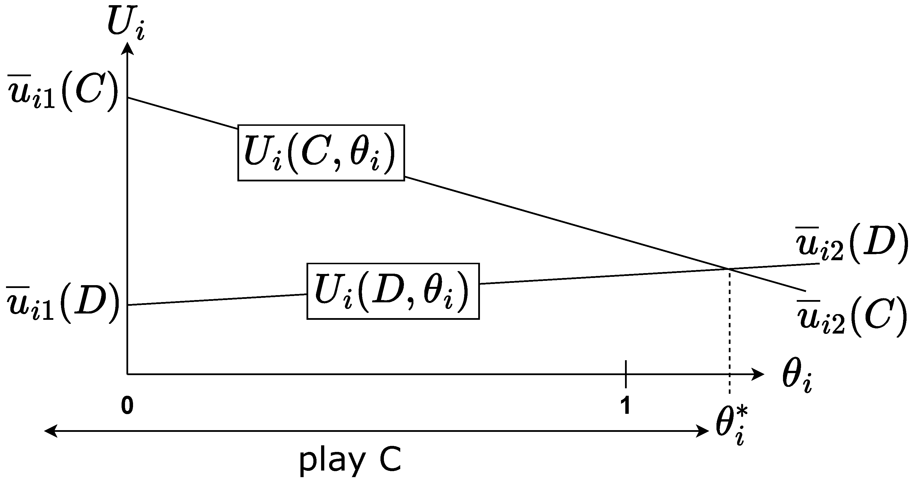
Note that for a given the expected values and are linear functions in , and they cross at since we have
As a result of this, we can formulate a more convenient definition for threshold strategy in the DGPD context.
Definition 10 (DGPD Threshold strategy).
A threshold strategy with threshold for agent i is a strategy such that
Again, by construction, the best response must be a threshold strategy as we have just rearranged the notation compared to the general definition. Note that when the pro-social coefficient is low (i.e., below the threshold), agent i defects, and when the pro-social coefficient is high (i.e., above the threshold), agent i cooperates. Figure 2 summarizes the concept of threshold strategy in the context of DGPD.

Figure 2.
DGPD strategy summarized ().
We define the threshold function using the following:
Using a simple calculation, we conclude that, given the other agent strategy , agent i’s best response is a threshold strategy with threshold .
We now define and that are combinations of DGPD payoff parameters as in (Edalat et al., 2018):
Proposition 2 ( monotonicity).
The threshold function is monotonic and is increasing if , decreasing if and is constant for .
Proof.
The monotonicity is straightforward. Then, we just note that and . □
Proposition 3.
For any DGPD with continuous type space and continuous prior, there exists a pure Bayesian Nash equilibrium. This equilibrium comprises threshold strategies with thresholds .
Proof.
The predicate results from the fact that and is monotonic in . □
2.5. Example for the SADP
Consider a simple situation with two companies, each having two different visions and two possible actions. Assume, for example, that the first vision is to protect the brand reputation and the second is to gain market shares. Suppose that there is an opportunity to establish a new production facility in a controversial area. Seizing the opportunity will for sure help gain market shares but will also impact negatively on the reputation. Each company can either leave this opportunity (C) or compete to set up a new site in the area (D). Table 3 and Table 4 summarize this situation:

Table 3.
Market share game.

Table 4.
Reputation game.
Both companies have a continuous type space and prior. According to our last result, there exists a pure Bayesian Nash equilibrium comprising threshold strategies. By computing and , we also know that the thresholds are in . If we add the assumption that priors are uniform, we can show (see Section 2.7 on Algorithmic results) that
2.6. Application to Other 2-Players Games
In this section, we present other examples of multigames for which we can apply our result on the existence of pure NE.
2.6.1. A Chicken Game Variation
In the game of chicken (also called the hawk–dove game) (Osborne & Rubinstein, 1994) there are two agents that can either pursue conflict (Conflict) or avoid it (Avoid). The best outcome for an agent is to play Conflict while the other plays Avoid. As opposed to the PD, if they both play Conflict, they both face the worst outcome. An example is given in Table 5.

Table 5.
The chicken game payoff matrix.
Because it is mainly a toy example like the PD, this game can only model very specific situations. We suggest that the game can be understood as a combination of two drivers: ego and survival. Under the ego consideration, we want to play Conflict to not be considered the “chicken”. It is important is to show that we dominate our opponent and have a stronger mind. Under the survival consideration, we mainly want to avoid the situation where both agents play Conflict. An example of both games is given in Table 6 and Table 7. The double game comprising those two games with continuous priors has a pure Nash equilibrium because the ego game has a strictly dominant strategy (Conflict).

Table 6.
Ego game.

Table 7.
Survival game.
2.6.2. A Battle of Sexes Variation
In the Battle of Sexes (also called Bach or Stravinsky), there are two agents that want to meet in an event but have opposed tastes (see Table 8). The main goal of both is to spend time together, but they also value going to the event they enjoy the most.

Table 8.
The Bach or Stravinsky payoff matrix.
As presented in the previous example, we can try to decompose considerations into taste and social considerations. In the taste game (Table 9) both agents are motivated to follow their taste no matter what the other does. In the social game (Table 10), the agents want to be at the same event, no matter which event it is.

Table 9.
Taste game.

Table 10.
Social game.
Like before, the double game comprising those two games with continuous priors has a pure Nash equilibrium because the taste game has a strictly dominant strategy (Bach for agent 1 and Stravinsky for agent 2).
2.6.3. An Assurance Game Variation
The assurance game (or Stag Hunt) is a two-player game involving a conflict between personal safety and social cooperation. An example of payoff matrix is given in Table 11. In essence, this game is very similar to the prisoner’s dilemma. Thus, we naturally combine it with a social game and obtain a variation of the DGPD.

Table 11.
The Stag Hunt payoff matrix.
2.7. Equilibrium Computation
2.7.1. Uniform Prior
Recall the definition of and that characterize the best response of an agent given its opponent’s strategy (assuming that they both follow a threshold strategy):
In the case of a uniform prior, . For simplicity, we use the notation and . Given that the opponent plays a threshold strategy with the threshold , we have
Therefore, we can rewrite the threshold function as a function of :
where
First, assume that the solution is symmetric for both players, meaning that :
which is reduced to
This is a quadratic equation. To evaluate the number of solutions we compute the discriminant:
If we search for non-symmetric solutions, the condition no longer holds. By performing the same kind of computation we end up with
This is also a quadratic equation, and we notice that it is the same quadratic as the symmetric case but multiplied by the constant . Hence, both equations have exactly the same solutions.
Proposition 4.
Proof.
The discriminant of those quadratics can be written as . From the constraints on the DGPD parameters, and , we thus have and the quadratics have two solutions and . □
Now, we need to check the validity of the solutions, i.e., .
Proposition 5.
Proof.
By computing and we can notice that depending on the sign of d, we have either or . In both cases, the solution is not valid. With the same kind of reasoning, we can show that depending on the sign of d, we have either or . Thus, is always valid. □
We end up with the fact that such games have always exactly one pure NE which is symmetric (i.e., both players have the same threshold) where .
2.7.2. General Solution
We denote by the cumulative distribution function of agent i’s prior . In the case of a uniform prior, we were able to explicitly find and deduce an algebraic equation for the solutions. To find a solution for any prior, we have to solve the following set of equations:
with
Therefore, for a continuous type space, the NE search is equivalent to solving a nonlinear multivariate equation:
3. Uniform Multigames with Discrete Type Space
3.1. General Remarks
The type space is now assumed to be discrete. The term , for , is the same as the continuous prior except that the integral is now replaced with a sum. Thus, we keep the same notations and consider
When there are only two actions, the notion of threshold strategy remains exactly the same; however, since the type space is discrete, two strategies with different thresholds can evaluate to the same value for types and actions .
Definition 11 (Equivalent strategies and thresholds).
Two strategies and for player are said to be equivalent () if
Given two threshold strategies and , and are said to be equivalent () if .
Notice that the binary relation ∼ restricted to threshold strategies is obviously an equivalence relation.
We also note that in contrast to the relation between strategies, the relation between thresholds is not an equivalence relation. Indeed, if a threshold leads to a mixed threshold strategy we cannot write because of Definition 7 is not constrained. In other words, two strategies with the same threshold can be different (as long as the mixed case is reached by some ). Note that a threshold strategy is mixed if and only if there exists such that .
Given a threshold strategy , let be the set of threshold strategies equivalent to . Given a threshold , let be the set of thresholds equivalent to .
Proposition 6.
Suppose that a threshold for leads to a pure threshold strategy (i.e., ). Then, we have the following properties:
- 1.
- is a non-empty set.
- 2.
- For any (strictly) positive , .
- 3.
- is a convex set.
- 4.
- If is finite, contains vectors that are not collinear with .
Proof.
1. We have ; thus, the latter set is non-empty.
- 2.
- Since the strategy only depends on the sign of , multiplying by a strictly positive has no impact on the resulting action.
- 3.
- Take , and , then notice that has the same sign as , so that .
- 4.
- Assume that is finite and consider and . Let :So, and have the same sign for any which concludes the proof.
□
3.2. The Double Game Prisoner’s Dilemma
We keep the same framework for the DGPD with a discrete type space. For each , we have
and
Proposition 7.
Consider agent i and let be two consecutive types from . All threshold strategies with a threshold such that are equivalent.
Proof.
This follows from the fact that there exists no type between and , so as long as we keep the threshold between those two values we end up with the same actions for agent i. □
Note that for threshold strategies, the third case () can only be reached if . So, if or , then the strategy is pure.
The search for a pure Nash equilibrium in the discrete case requires a different method since we do not have a general result for two-action multigames that can be used as in the case of continuous type space. To go further, we assume that the type space is finite. Recall for player i that is the probability that the other agent’s action is given that it follows .
Proposition 8 ( monotonicity).
Consider agent i and suppose that the other agent follows a threshold strategy with threshold . This threshold strategy induces a value for agent i. If the other agent changes its strategy by increasing its threshold , then the induced value decreases.
Proof.
By increasing its threshold value, agent decreases the probability of playing C and thus decreases the value
□
For integers with , let denote the set of integers, .
Lemma 1.
Suppose and are both increasing (or both decreasing). Then, there exists such that .
Proof.
We first notice that is increasing and for . Hence, there exists a least non-negative integer k such that and it follows that . □
Theorem 5.
For any DGPD with finite type space there exists a pure Bayesian Nash equilibrium comprising threshold strategies such that for both agents, the threshold .
Proof.
We suppose that (the reasoning for is similar). Suppose that agent plays a threshold strategy . Then, the agent i’s best response is also a threshold strategy . By the monotonicity of and (Propositions 2 and 8), if agent increases its threshold then the threshold of agent i’s best response also increases (if then agent i’s best response threshold decreases).
Now, consider the partition of into intervals according to agents’ type spaces:
For agent i’s threshold strategy and agent ’s best response , there exists (1) such that and (2) such that . Note that if , then it belongs to two adjacent intervals and . In this case, we arbitrarily choose to take .
We define the transition functions and such that . In order to show that there exists a pure Nash equilibrium, we need to show that
Equivalently, we search for such that . From Lemma 1 with and as f and g, we can find a solution . □
3.3. Example
Suppose that G is a double game prisoner’s dilemma with a uniform prior such that utilities for both agents are given according to Table 12 and Table 13 and type space for . We obtain and (represented in Figure 3).

Table 12.
Utilities for the first game.

Table 13.
Utilities for the second game.
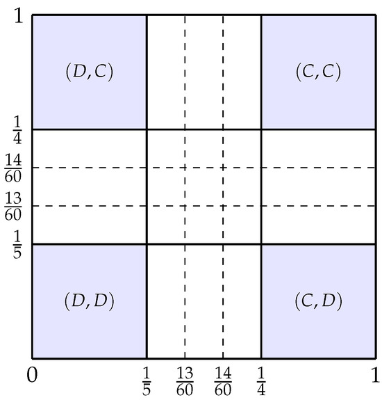
Figure 3.
Representation of both agent’s type space.
To find a pure Bayesian NE, one has to find a pair of threshold strategies such that is the best response to and is the best response to . From the symmetry of the game, we can expect that (i.e., they have the same threshold). We have
while can take three different values:
Possible values for are , or . Those three values are in the interval . So, the pair where
is a pure (Bayesian) strategy Nash equilibrium for the game G.
3.4. On a Simple Multigame Classification
In this section, we consider multigames with finite type space. Both actions are still denoted by C and D (even if they are not necessarily associated to cooperation or defection). The payoff matrix U is not constrained as opposed to DGPD configuration. First, we define a simple classification of such games according to properties of U.
Definition 12.
We denote the type space configuration by . Any payoff matrix U belongs to one of the following sets:
- 1.
- The full set: payoff matrices U such that for any type space configuration the game has a pure Nash equilibrium.
- 2.
- The solutionless set: payoff matrices U such that for any type space configuration the game has no pure Nash equilibrium.
- 3.
- The hybrid set: payoff matrices U such that the existence of a pure NE for depends on the type space configuration.
Proposition 9.
The full set is not empty: it contains matrices U with the DGPD payoff constraints. The hybrid set is also not empty.
Proof.
The first set is obviously not empty in view of Theorem 5. The second set is not empty as we can find G and sharing the same payoff matrix such that one has a pure NE and the other not (see next examples). □
Consider the uniform double game G with utilities for agents given by Table 14 with type space , and the prior , such that

Table 14.
Utilities for both basic games.
This game has no pure Bayesian Nash equilibrium. Consider a slight variation of the game G such that utilities for agents are given by Table 14 with type space , and the prior , such that
Consider as a C/D threshold strategy with and as a C/D threshold strategy with . The pair is a pure Bayesian Nash equilibrium for the game .
Note that we do not give any particular property for the solutionless set. We postulate that this set is empty (see Section 3.5 on algorithmic results). Recall the following formulae for the configuration:
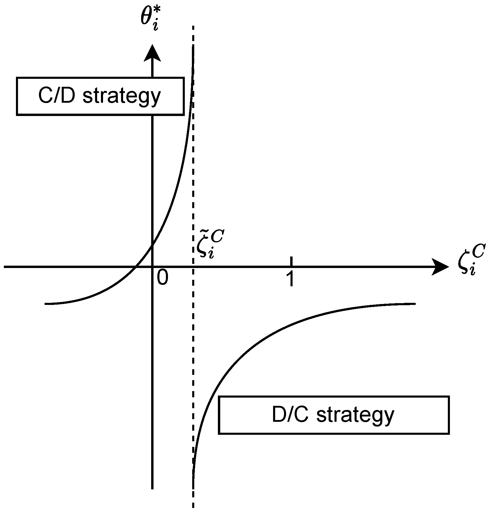
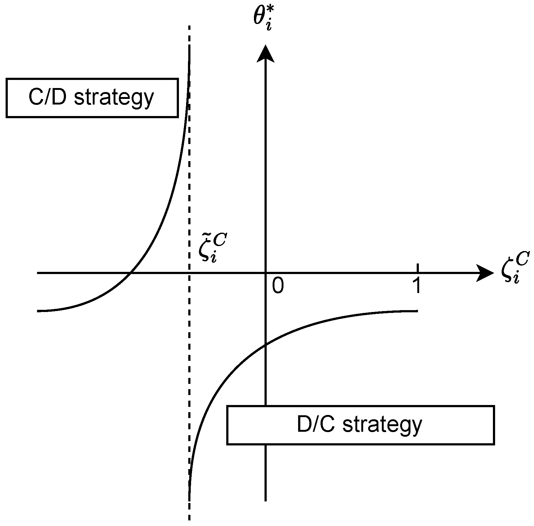
Observe that with no assumption on the payoff matrix, there is no guarantee that and will cross for a given . Moreover, the crossing point (if it exists) is not guaranteed to be inside as illustrated by Figure 4 and Figure 5. It cuts into two regions, one in which the best action is C and the other in which the best action is D. If the left region is C then the resulting strategy is a C/D strategy (Figure 4) and if the left region is D then the resulting strategy is a D/C strategy (Figure 5). We call this the strategy type. For any DGPD configuration, the best response is always a D/C strategy.
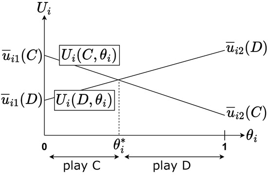
Figure 4.
Crossing point (threshold) inside .
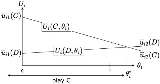
Figure 5.
Crossing point outside .
As with the DGPD, we define the threshold function for agent i:
When , both utility functions have the same slopes and the threshold function is not defined. As long as , utility functions are not equal; so, there is one best action (either C or D). In this case, the best response is also a threshold strategy with the threshold . Otherwise, both utility functions are equal (there is an infinite number of crossing points). Because of the latter case, we can no longer state that any best response comprises threshold strategies.
Definition 13 (D/C threshold strategy).
A threshold D/C strategy with threshold for agent i is a strategy such that
Now, we can express the threshold as a function of instead of :
The case of equal slopes is reached at the forbidden value :
Therefore, the case of equal utility functions happens when
We notice that the graph of is split into two regions by the forbidden value (Figure 6 and Figure 7). Each region is associated with a different strategy type. Thus, if is not in , then agent i will always play the same strategy type notwithstanding its opponent’s strategy. In Figure 7, the forbidden value is outside , so agent i will only play a D/C strategy. In Figure 6, the forbidden value is in , so agent i may play both strategy types depending on the opponent’s strategy : if then agent i plays a C/D strategy and if then agent i plays a D/C strategy. Suppose that for . Both agents always stick to the same strategy type and there are three cases: (1) both play C/D, (2) both play D/C (like the DGPD), and (3) one plays C/D while the other plays D/C.

Figure 6.
Forbidden value inside .

Figure 7.
Forbidden value outside .
In order to characterize the variations of , define
Proposition 10
( monotonicity). The threshold function is monotonic and satisfies the following
- 1.
- if then is increasing,
- 2.
- if then is decreasing,
- 3.
- if then is constant.
Proof.
Simply compute the derivative of the function which is a homography and obtain the condition on . □
Proposition 11.
Let U be the payoff matrix of a two-player double game such that
- 1.
- for where is the forbidden value of ,
- 2.
- and have the same sign if both agents play the same strategy type or have opposite sign otherwise.
Then, for any type space configuration the game has a pure Bayesian Nash equilibrium.
Proof.
The two conditions imply that (1) agents have a unique strategy type and (2) their best response threshold functions have the same monotonicity, i.e., increasing or decreasing. Thus, we can follow the same reasoning as we had for DGPD to prove the existence of a pure Bayesian NE. □
3.5. Algorithmic Results
In this section, we develop efficient algorithms to find pure Bayesian Nash equilibria for finite type space . The first part focuses on an optimized version for DGPD while the second one focuses on a more general version. In the third part, the complexity of both algorithms are evaluated and compared to each other.
3.5.1. Algorithm for DGPD
Recall that the agents’ best response sets only comprise threshold strategies. Thus, given a finite type space (with elements for agent i) the search space comprises threshold strategy pairs. The pure Bayesian Nash equilibrium search consists of finding a fixed point (two strategies that are the mutual best responses of each other) among those combinations.
For clarity, we formulate a graphical method to represent the solution search that we call a strategy diagram that looks like Figure 8. There are two unit intervals , one for each agent’s type space. An arrow from agent i’s interval to agent ’s interval indicates that if agent i plays a threshold strategy with a threshold in , the best response of agent is a threshold strategy with a threshold in . A solution is then simply represented by two compatible arrows as displayed in Figure 9.
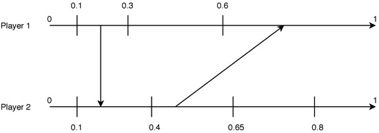
Figure 8.
If agent 1 plays a threshold strategy with , agent 2’s best response is a threshold strategy with .

Figure 9.
A pure Bayesian NE represented by compatible arrows.
We now introduce Algorithm 1 for NE search on finite DGPD. For every threshold strategy of agent 1, we compute the associated best response of agent 2 and then compute the best response of agent 1 given the latter. Whenever for any of agent 1’s threshold strategy the computed best response is equivalent, we obtain a pure NE. The procedure compute_cumul_proba() returns the cumulative probabilities given a probability distribution. finder() returns the index of the type space interval that contains a given threshold. search_space_boundaries() computes and and then the associated indices in the type space. This helps us optimize the overall algorithm by reducing the search space to thresholds . Finally, threshold_i() is the threshold function of agent i.
| Algorithm 1 Exhaustive NE search |
| Require: for do if then return , end if end for return False |
Figure 10 and Figure 11 illustrate the finding of NE search for two situations that we encounter. Note that when we reverse the second agent’s axis as the best response threshold monotonicity is reversed compared to . Also note that there could be multiple solutions (Figure 11). If we only seek one solution then we stop at the first finding to reduce the computational cost.

Figure 10.
Strategy diagram when .

Figure 11.
Strategy diagram when .
3.5.2. General Algorithm
We now describe a different algorithm that can handle a broader range of games but is more expensive. It can also handle DGPD games but is computationally less efficient as it explores a larger search space without exploiting the DGPD structure.
Apart from the fact that we have to explore both C/D and D/C strategies, the double game algorithm is very similar to the DGPD algorithm. For each type space interval of agent 1, we compute the best response of agent 2 and the best response of agent 1 given the latter. We check that we fall back to the initial strategy by ensuring that the thresholds are in the same interval and that the strategy types are the same. Of course, we cannot benefit from the reduced search space with and as they make no sense in the general context. The overall procedure is summarized in Figure 12.

Figure 12.
Search process for the discrete double game.
Given this general algorithm we explore some properties of payoff matrices. We generated hundreds of random payoff matrices and thousands of type space configurations and ran Nash equilibrium searches. We experimentally classified the payoff matrices thanks to the NE search results. Interestingly, we notice that none of the generated matrices belongs to the solutionless set as we postulated earlier. Secondly, we find that there exist matrices in the full set that do not satisfy the conditions of Proposition 11: the set of conditions is sufficient, but not necessary, for belonging to the full set.
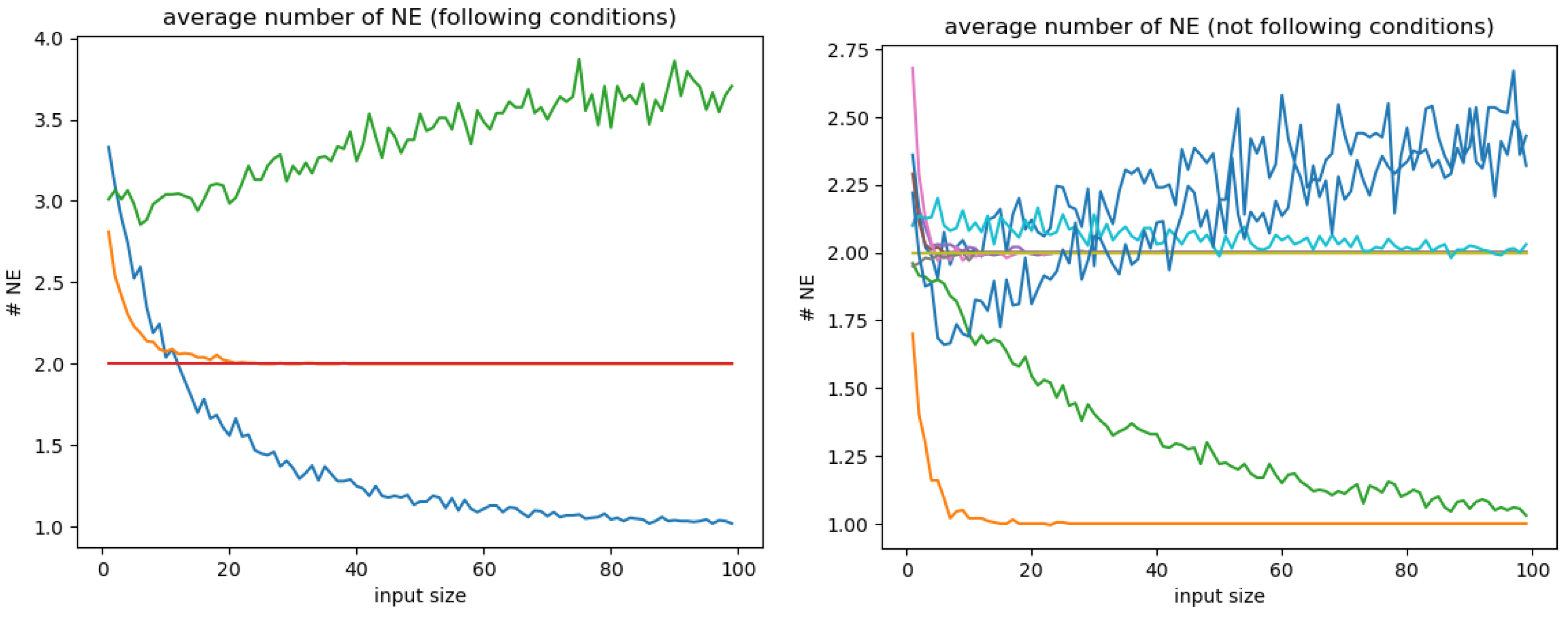
Next, using a modified version of the NE search that does not stop at the first solution (if it exists) we computed the average number of solutions for different type space configurations. Let input size denote the number of elements in the type space for both players. In this context, and .
Figure 13 shows the results for a sample of payoff matrices randomly chosen from the full set (thanks to our previous classification). The first trivial result is that the average never goes under 1 (otherwise it would not belong to the full set). Secondly, it seems that the average number of solution can either be constant, increase or decrease with the input size. In many cases, we even observe that the average number tends to stabilize around an arbitrary value which seems to be an integer.

Figure 13.
Average number of solutions with respect to the input size of both agents. Each curve corresponds to a payoff matrix. Among matrices belonging to the full set, we distinguish those satisfying the conditions of Proposition 11 (left) from those not satisfying them (right).
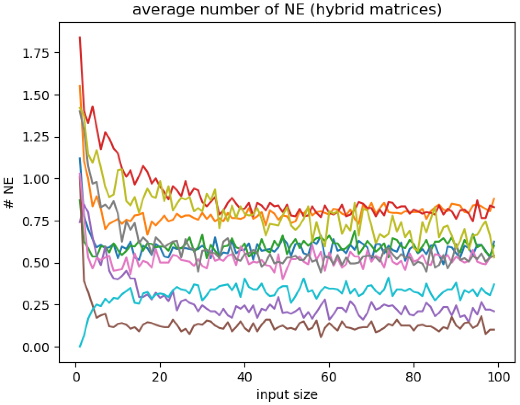
We repeated this experiment with payoff matrices randomly picked from the hybrid set. Figure 14 shows a sample of results for such matrices. As we said earlier for the full set, it seems that the averages can either increase, decrease, or stay constant and that they converge to different values. This time, those values are smaller than 1 and may not be integers.

Figure 14.
Average number of solutions with respect to the input size of both agents. Each curve corresponds to a payoff matrix from the hybrid set.
3.5.3. Complexity Comparison
In this section, we discuss the complexity of each algorithm and compare their performances.
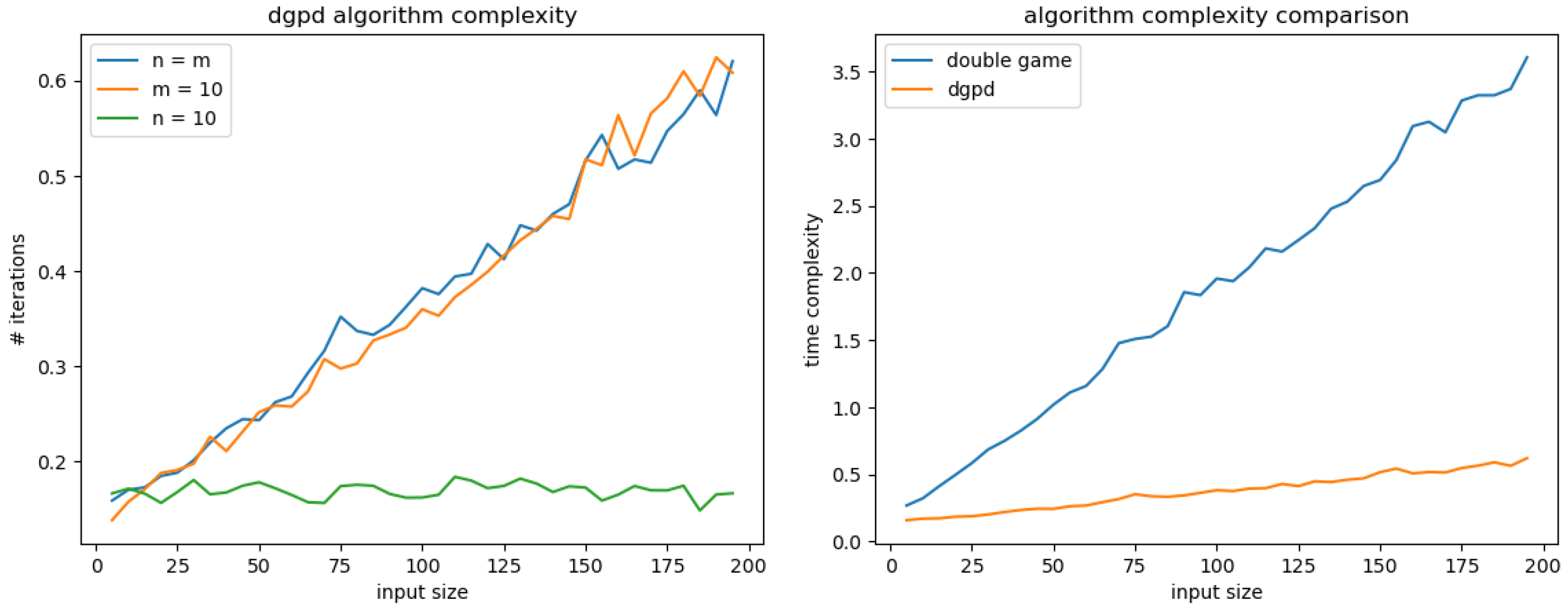
First of all, the left part of Figure 15 displays the complexity of DGPD NE search for different variations of inputs. When , both input sizes vary, while when or only input size varies. Notice that when the first agent’s input size is constant, the complexity is also constant. When n varies, the complexity is linear and is almost independent of whether m varies or not. In fact, the main driver of the complexity is the main loop that iterates over the elements of . The procedure finder() has a low computational cost as it comprises a binary search. In practice, for imbalanced type space size, one should always consider the agent having the smallest type space as the first agent.
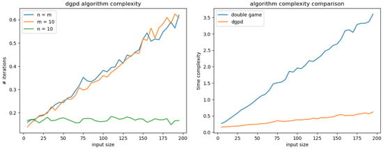
Figure 15.
DGPD time complexity (left) and comparison with general algorithm (right).
The right part of Figure 15 illustrates the improved performance of DGPD specific algorithm over the more general one. The latter also has a linear complexity but with a much higher slope. One explanation comes from the fact that for each element of we consider both C/D and D/C strategies as starting points. Also, we do not reduce the search space with bounds like and .
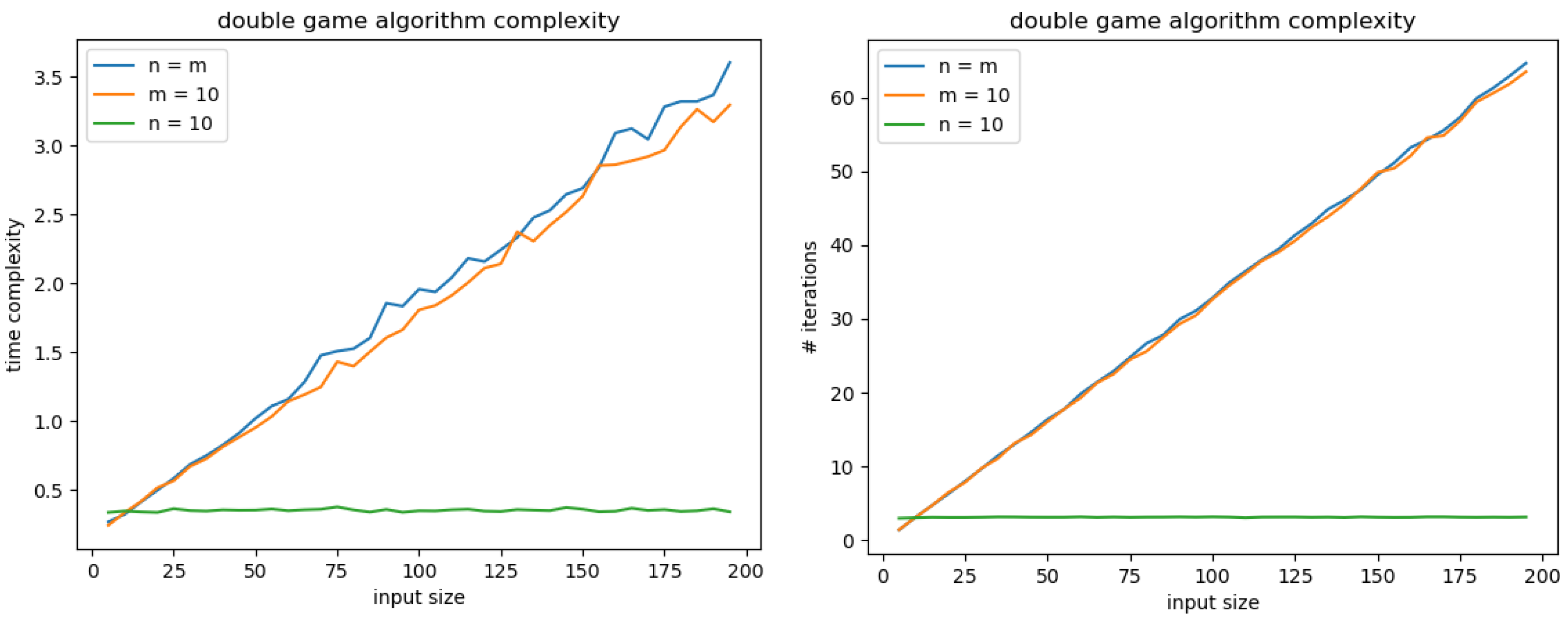
For the general algorithm, we also compare the complexity for different variations in the input size as display in Figure 16 (left). Again, the complexity heavily relies on the first agent’s type space size. In contrast to the DGPD algorithm, we notice that for the complexity is slightly below the complexity when . On the right side of Figure 16 we see that this behavior cannot be explained by a difference in the number of iterations on the main loop. It is probably due to the cost of finder() that increases in when m increases. This effect might also affect the DGPD algorithm but is not significant in our experiment.
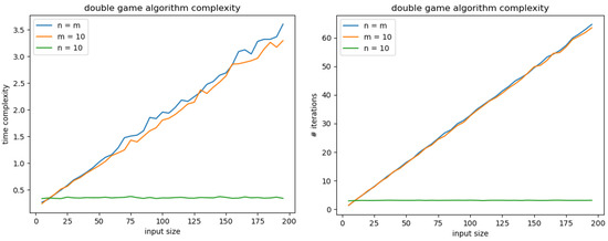
Figure 16.
Complexity comparison for different input sizes through computation time (left) and average number of iterations (right).
4. Conclusions
In this paper, we explored pure Bayesian Nash equilibrium existence for a subset of uniform multigames. We made the distinction between games according to their type space, either continuous or discrete.
For continuous type space games with two actions, we showed in Theorem 4 the existence of a pure Bayesian Nash equilibrium when there are local games having a strictly dominant strategy for each agent. We illustrated its application through the DGPD and SDAP examples that can model real situations with more precision than toy examples usually presented. In Section 2.7 we formulated a methodology to solve two-action games with any kind of prior.
For finite type space DGPD, we showed in Theorem 5 the existence of a pure Bayesian Nash equilibrium. Following this, we were able to provide efficient algorithms to find pure Bayesian Nash equilibrium and explore experimentally our classification of discrete double multigames (Proposition 11).
Threshold strategy is a core concept developed for both the continuous and the discrete type space games with two actions. As we saw, a threshold strategy is fully characterized by its threshold and defines three regions in the type space: one associated to a pure action C, one associated to a pure action D, and one associated to a mix. By construction, the best response must be a threshold strategy. The threshold strategies presented for the DGPD are the more basic version where we play D if , play C if , and a mix of both if .
As for future work, we could try to extend this notion to more than two actions. In this case, we would consider the to determine the action played by agent i with type . When the highest value is reached by two or more actions , the response of agent i would be a mixed combination of such actions. This definition would still use the fact that a Nash equilibrium solution (be it pure or mixed) must comprise threshold strategies.
Author Contributions
Conceptualization, A.E.; formal analysis, S.H.; investigation, S.H.; methodology, S.H.; software, S.H.; supervision, A.E.; validation, A.E. and S.H.; visualization, S.H.; writing—original draft preparation, S.H.; writing—review and editing, A.E. and S.H. All authors have read and agreed to the published version of the manuscript.
Funding
This research received no external funding.
Data Availability Statement
The algorithms presented in the study are openly available in GitHub on the repository https://github.com/huot-s/pure_ne_multigames (accessed on 3 July 2025). No new data were created or analyzed in this study.
Acknowledgments
We would like to thank Samira Hossein Ghorban https://orcid.org/0000-0003-4147-3181 (accessed on 3 July 2025) for helping us design some of the examples displayed in this article, in particular, the one in Section 3.3.
Conflicts of Interest
The authors declare no conflicts of interest.
Abbreviations
The following abbreviations are used in this manuscript:
| DGPD | Double-Game Prisoner’s Dilemma |
| SADP | Sustainable Adoption Decision Problem |
| NE | Nash Equilibrium |
| PD | Prisoner’s Dilemma |
| PPAD | Polynomial Parity Arguments on Directed graphs |
| C | Cooperation |
| D | Defection |
References
- Athey, S. (2001). Single crossing properties and the existence of pure strategy equilibria in games of incomplete information. Econometrica Wiley, Econometric Society. Available online: http://www.jstor.org/stable/2692247 (accessed on 3 July 2025).
- Carrozzo Magli, A., Posta, P. D., & Manfredi, P. (2021). The tragedy of the commons as a prisoner’s dilemma. its relevance for sustainability games. Sustainability, 13(15), 8125. [Google Scholar] [CrossRef]
- Daskalakis, C., Goldberg, P. W., & Papadimitriou, C. H. (2009). The complexity of computing a Nash equilibrium. SIAM Journal on Computing, 39(1), 195–259. [Google Scholar] [CrossRef]
- Dresher, M. (1970). Probability of a pure equilibrium point in n-person games. Journal of Combinatorial Theory, 8(1), 134–145. [Google Scholar] [CrossRef]
- Edalat, A., Ghorban, S. H., & Ghoroghi, A. (2018). Ex post Nash equilibrium in linear Bayesian games for decision making in multi-environments. Games, 9(4), 85. [Google Scholar] [CrossRef]
- Edalat, A., Ghoroghi, A., & Sakellariou, G. (2012). Multi-games and a double game extension of the prisoner’s dilemma. arXiv, arXiv:12.05.4973. [Google Scholar]
- Einy, E., & Haimanko, O. (2023). Pure-strategy equilibrium in Bayesian potential games with absolutely continuous information. Games and Economic Behavior, 140, 341–347. [Google Scholar] [CrossRef]
- Flood, M. M. (1958). Some experimental games. Management Science, 5(1), 5–26. [Google Scholar] [CrossRef]
- Friede, G., Busch, T., & Bassen, A. (2015). ESG and financial performance: Aggregated evidence from more than 2000 empirical studies. Journal of Sustainable Finance and Investment, 5, 210–233. [Google Scholar] [CrossRef]
- Friedman, D. (1998). On economic applications of evolutionary game theory. Journal of Evolutionary Economics, 8(1), 15–43. [Google Scholar] [CrossRef]
- Granovetter, M. (1978). Threshold models of collective behavior. American Journal of Sociology, 83, 1420–1443. [Google Scholar] [CrossRef]
- Hardin, G. (1968). The tragedy of the commons. Science, 162(3859), 1243–1248. [Google Scholar] [CrossRef]
- Harsanyi, J. C. (1967). Games with incomplete information played by “Bayesian” players, i-iii. part i. the basic model. Management Science, 14(3), 159–182. [Google Scholar] [CrossRef]
- Harsanyi, J. C. (1968a). Games with incomplete information played by “Bayesian” players, i-iii. part ii. Bayesian equilibrium points. Management Science, 14(5), 320–334. [Google Scholar] [CrossRef]
- Harsanyi, J. C. (1968b). Games with incomplete information played by “Bayesian” players, i-iii. part iii. the basic probability distribution of the game. Management Science, 14(7), 486–502. [Google Scholar] [CrossRef]
- Harstad, B. (2012). Climate contracts: A game of emissions, investments, negotiations, and renegotiations. The Review of Economic Studies, 79, 1527–1557. [Google Scholar] [CrossRef]
- He, W., & Sun, Y. (2019). Pure-strategy equilibria in Bayesian games. Journal of Economic Theory, 180, 11–49. [Google Scholar] [CrossRef]
- Heal, G., & Kunreuther, H. (2011). Tipping climate negotiations. National Bureau of Economic Research. [Google Scholar] [CrossRef]
- Krishna, V., & Perry, M. (1998). Efficient mechanism design. Hebrew University of Jerusalem. [Google Scholar]
- Larson, J. M. (2021). Networks of conflict and cooperation. Annual Review of Political Science, 24(1), 89–107. [Google Scholar] [CrossRef]
- Luenberger, D. G. (1998). Investment science. Oxford University Press. [Google Scholar]
- Manelli, A. M., & Vincent, D. R. (2007). Multidimensional mechanism design: Revenue maximization and the multiple-good monopoly. Journal of Economic Theory, 137, 153–185. [Google Scholar] [CrossRef]
- Martimort, D. (2010). Multi-Contracting mechanism design. In Advances in economics and econometrics: Theory and applications, ninth world congress (Volume I). Cambridge University Press. [Google Scholar] [CrossRef]
- McAdams, D. (2003). Isotone equilibrium in games of incomplete information. Econometrica Wiley, Econometric Society. Available online: http://www.jstor.org/stable/1555494 (accessed on 3 July 2025).
- Milgrom, P., & Shannon, C. (1994). Monotone comparative statics. Econometrica Wiley, Econometric Society. Available online: http://www.jstor.org/stable/2951479 (accessed on 3 July 2025).
- Monderer, D., & Shapley, L. S. (1996). Potential games. Games and Economic Behavior, 14(1), 124–143. [Google Scholar] [CrossRef]
- Nordhaus, W. (2015). Climate clubs: Overcoming free-riding in international climate policy. American Economic Review, 105, 1339–1370. [Google Scholar] [CrossRef]
- Osborne, M. J., & Rubinstein, A. (1994). A course in game theory (Vol. 1). The MIT Press. ISBN 9780262650403. [Google Scholar]
- Papadimitriou, C. H. (1994). On the complexity of the parity argument and other inefficient proofs of existence. Journal of Computer and System Sciences, 48(3), 498–532. [Google Scholar] [CrossRef]
- Pástor, Ľ., Stambaugh, R. F., & Taylor, L. A. (2021). Sustainable investing in equilibrium. Journal of Financial Economics, 142, 550–571. [Google Scholar] [CrossRef]
- Porter, M. E., & Kramer, M. R. (2011). Creating shared value. Harvard Business Review, 89, 4–5. [Google Scholar]
- Poundstone, W. (1993). Prisoner’s dilemma: John von neumann, game theory, and the puzzle of the bomb. Knopf Doubleday Publishing Group. ISBN 0-385-41580-X. [Google Scholar]
- Rabinovich, Z., Naroditskiy, V., Gerding, E. H., & Jennings, N. R. (2013). Computing pure bayesian-nash equilibria in games with finite actions and continuous types. Artificial Intelligence, 195, 106–139. [Google Scholar] [CrossRef]
- Reny, P. J. (2011). On the existence of monotone pure-strategy equilibria in bayesian games. Econometrica Wiley, Econometric Society. Available online: http://www.jstor.org/stable/41057464 (accessed on 3 July 2025).
- Rinott, Y., & Scarsini, M. (2000). On the number of pure strategy nash equilibria in random games. Games and Economic Behavior, 33(2), 274–293. [Google Scholar] [CrossRef][Green Version]
- Shapiro, C. (1989). The theory of business strategy. The Rand Journal of Economics, 20(1), 125–137. [Google Scholar] [CrossRef]
- Stanford, W. (1995). A note on the probability of k pure nash equilibria in matrix games. Games and Economic Behavior, 9(2), 238–246. [Google Scholar] [CrossRef]
- Stanford, W. (1997). On the distribution of pure strategy equilibria in finite games with vector payoffs. Mathematical Social Sciences, 33(2), 115–127. [Google Scholar] [CrossRef]
- Stanford, W. (1999). On the number of pure strategy nash equilibria in finite common payoffs games. Economics Letters, 62(1), 29–34. [Google Scholar] [CrossRef]
- Stern, N. (2007). The economics of climate change: The stern review. Cambridge University Press. [Google Scholar]
- Székely, T., Moore, A. J., & Komdeur, J. (2010). Social behaviour: Genes, ecology and evolution. Cambridge University Press. [Google Scholar]
- van den Assem, M. J., van Dolder, D., & Thaler, R. H. (2011). Split or steal? cooperative behavior when the stakes are large. Management Science, 58, 2–20. [Google Scholar] [CrossRef]
- von Neumann, J., & Morgenstern, O. (1944). Theory of games and economic behavior. John Wiley and Sons. [Google Scholar]
Disclaimer/Publisher’s Note: The statements, opinions and data contained in all publications are solely those of the individual author(s) and contributor(s) and not of MDPI and/or the editor(s). MDPI and/or the editor(s) disclaim responsibility for any injury to people or property resulting from any ideas, methods, instructions or products referred to in the content. |
© 2025 by the authors. Licensee MDPI, Basel, Switzerland. This article is an open access article distributed under the terms and conditions of the Creative Commons Attribution (CC BY) license (https://creativecommons.org/licenses/by/4.0/).


