A Generalization of Quantal Response Equilibrium via Perturbed Utility ^†

Abstract

We present a tractable generalization of quantal response equilibrium via non-expected utility preferences. In particular, we introduce concave perturbed utility games in which an individual has strategy-specific utility indices that depend on the outcome of the game and an additively separable preference to randomize. The preference to randomize can be viewed as a reduced form of limited attention. Using concave perturbed utility games, we show how to enrich models based on logit best response that are common from quantal response equilibrium. First, the desire to randomize can depend on opponents’ strategies. Second, we show how to derive a nested logit best response function. Lastly, we present tractable quadratic perturbed utility games that allow complementarity.

1. Introduction

This paper generalizes quantal response equilibrium (QRE) using the standard Nash equilibrium concept via the class of concave perturbed utility games (PUGs). QRE, as studied in [1,2], assumes that individuals maximize expected utility, but that there is an unobserved additive random shock to a base utility index that drives deviations from Nash equilibrium behavior. In contrast, PUGs specify a deterministic non-expected utility function with a preference for randomization that is additively separable from a base utility index. Here, the preference for randomization can be viewed as a reduced form of limited attention. While these approaches seem different, any QRE can be modeled as a Nash equilibrium of a concave perturbed utility game.1 PUGs also generalize the control costs approach of van Damme [6,7].2

Using the Nash equilibrium concept with the more general concave PUGs is useful compared to QRE since it is often difficult to select a distribution of tractable additive random shocks. PUGs facilitate estimation of model parameters via standard maximum likelihood methods (without numerical integration). Moreover, PUGs allows complementarity between strategies which is not allowed in any QRE. PUGs also can easily incorporate that the probability an individual chooses a strategy as a best response also depends on how likely opponents play their strategies. Importantly, any concave PUG has a Nash equilibrium as an immediate corollary of Debreu [8]. This existence result allows us to generate different flavors of the logit best response, derive a nested logit best response function, and discuss quadratic perturbed utility games.

The result that QRE can be represented as Nash equilibria of a non-expected utility game matters for interpretation and has practical implications. Concerning interpretation, violations of standard Nash play can be interpreted either as errors of individual perception or as the manifestation of a non-expected utility preference. These two interpretations have different implications for welfare analysis. For example, one may not want perceptual errors to enter welfare calculations but may want to include all facets of a non-expected utility preference in welfare calculations. On the practical side, it may be easier to place restrictions on perturbation functions than restricting the additive error term of QRE since analytical results for integrating error distributions are known only in some special cases. In contrast, rich classes of analytical perturbation functions are studied in [9,10]. These perturbation functions can be seen as generalizations of the entropy function that is often used to study limited attention.

We mention a non-extensive summary of related work. A perturbed utility game is similar to the control costs approach developed in [6,7] whereby there is a cost associated to the ability to control a “tremble.” Control costs are assumed to be additively separable, whereas perturbed utility games have costs that are nonseparable and can depend on the opponents’ strategies. Rosenthal [11] considered a related approach of bounded rationality where the probability of choosing an action is monotone with utility. Voorneveld [12] showed that the solution concept in [11] can be represented with quadratic control costs or a quantal response equilibrium with uniform errors. Stahl [13] looked at a game with trembles and an entropic cost to control the trembles. Mattsson and Weibull [14] gave axioms for entropic control functions for individual decisions and deals with a continuum of alternatives. With regards to QRE, the regular quantal response equilibrium of Goeree et al. [15] places additional assumptions on QRE and a textbook treatment of QRE is available in [16].3 We also note that recent work by Melo [18] examines uniqueness properties of quantal response equilibrium while using a perturbed utility game as an intermediate step.

We also briefly describe some history regarding non-expected utility games and QRE. Shortly after the study of individual non-expected utility functions in [19], there was some interest to study non-expected utility in strategic games following those in [20,21]. For example, equilibrium concepts, existence of equilibria, and dynamic consistency properties when individuals do not satisfy the independence axiom are studied in [22,23]. However, there is little applied work that resulted from this research. In contrast, quantal response equilibria was developed a few years later by the authors of [1,2], and has been extensively used in applications to account for deviations from Nash equilibrium. By linking these two approaches, we show applied researchers that Nash equilibrium with non-expected utility preferences provides a rich and tractable avenue to account for deviations from Nash equilibrium with expected utility preferences.

Finally, PUGs model individuals with a deterministic preference for randomization following Machina [24] and relate more broadly to the stochastic choice literature.4 We say an individual has a preference for randomization when the individual plays the game as if they randomize their play according to a most-preferred distribution of pure strategies. We assume throughout that individuals commit to randomize according to their most-preferred distribution.5 While a preference for randomization may seem foreign, there is growing experimental evidence that supports this interpretation [34,35,36,37,38,39,40,41]. The most important finding for our purposes is that of Agranov et al. [41], who found that individuals who randomize choices in individual decision problems also randomize their choices in strategic environments. Therefore, it may be important to account for a preference of randomization in games.

The rest of this paper is organized as follows. Section 2 describes the structure of a concave perturbed utility game and shows existence of equilibria for all such games. Section 3 derives the logit best response function from a concave perturbed utility game with entropy costs and discusses various flavors of the logit best response. Section 4 examines other forms of concave perturbed utility games. In particular, we examine nested logit equilibria and discusses quadratic perturbed utility games. Section 5 provides an example game and graphs best responses for various perturbed utility functions. We give our final remarks in Section 6. The proofs are mathematically simple, but included in the Appendix A for completeness.

2. Concave Perturbed Utility Games and Existence

Consider a finite N-player game with a set $\{1,\dots ,N\}$ of players. Each player $n\in \{1,\dots ,N\}$ has a set of pure strategies given by $S_n=\{s_{n,1},\dots ,s_{n,J_n}\}$ where $J_n$ is the number of pure strategies for the nth player. Let a pure strategy profile be defined by $s=(s_1,\dots ,s_n)\in S={\prod }_{n=1}^N{S}_n$ where S is the set of all pure strategy profiles. Occasionally, it is useful to represent a strategy profile by $s=(s_n,s_{-n})$ where $s_n$ is the strategy of the nth player while $s_{-n}$ contains the pure strategies taken by all other players where $s_{-n}\in S_{-n}={\prod }_{m\ne n}{S}_m$.

Let ${\Delta }_n$ be the set of probability measures on $S_n$. We represent elements of ${\Delta }_n$ by $p_n\in {\Delta }_n=\{p_n\in {\mathbb{R}}^{J_n}\mid \mathrm{for}\mathrm{all}j\in J_n,p_{n,j}\ge 0\mathrm{and}{\sum }_{j=1}^{J_n}{p}_{n,j}=1\}$. The element $p_n\in {\Delta }_n$ is a mixed strategy for the nth player. Here, $p_{n,j}$ is the probability the nth agent plays their jth strategy $s_{n,j}$. Further, let all mixed strategy profiles be given by $\Delta ={\prod }_{n=1}^N{\Delta }_n$ where a mixed strategy profile is given by $p=(p_1,\dots ,p_N)\in \Delta$. We use the shorthand $p=(p_n,p_{-n})$ to denote a mixed strategy profile where the nth player plays the mixed strategy $p_n$ and all other agents play their corresponding mixed strategy in $p_{-n}\in {\Delta }_{-n}={\prod }_{m\ne n}{\Delta }_m$.

We assume there are observed outcomes for each player $n\in \{1,\dots ,N\}$ that depend on the strategy profile $s\in S$ denoted by $x_{n,s}\in X_n$. For example, $X_n$ could be monetary outcomes that depend on the strategies of all players. If an individual has social preferences and cares about other individuals, then $X_n$ could be the monetary allocations to all individuals. This means that a motive for cooperation can be modeled in this framework. Finally, $X_n$ could be a consumption bundle. For example, if each pure strategy is to bring an item to a picnic, then $X_n$ could be the space of ordered tuples of consumption goods. Thus, we view the outcome of a game as covariates similar to in [42,43,44].

We let $x_n={\left(x_{n,s}\right)}_{s\in S}$ denote the vector of the nth player’s outcomes for all strategy profiles. Let $x=(x_1,\dots ,x_N)$ denote the collection of all individual observable outcomes. We use the notation $x_n^j={\left(x_{n,(s_{n,j},s_{-n})}\right)}_{s_{-n}\in S_{-n}}$ to denote the vector of outcomes the nth player can obtain for all other combinations of opponent pure strategies when their jth strategy is played. The different values of the outcomes are mapped into a utility index that depends on opponent mixed strategies.

We consider non-expected utility preferences for each player $n\in \{1,\dots ,N\}$ given by the class of concave perturbed utility preferences. In particular, the nth player has preferences represented by the non-expected utility function given by

$$\sum _{j=1}^{J_n}{p}_{n,j}{U}_{n,j}(p_{-n},x_n^j)+D_n(p_n,p_{-n}).$$

Here, $U_{n,j}:{\Delta }_{-n}\times X_n^{|S_{-n}|}\to \mathbb{R}$ is a utility index that captures the attractiveness of the nth player’s jth strategy that is assumed continuous in $p_{-n}$ and depends on the outcomes associated with the nth player’s jth strategy. The function $D_n:{\Delta }_n\times {\Delta }_{-n}\to \mathbb{R}$ is assumed concave in $p_n$ for every $p_{-n}$ and jointly continuous in $(p_n,p_{-n})$. We call $D_n$ the nth individual’s perturbation function. The perturbed utility approach differs from the control function approach of van Damme [7] since the attractiveness of a pure strategy can depend on the play of opponents and the preference for randomization can also depend on the play of opponents.

The usual expected utility conditions are expressed when the nth individual evaluates the value of the jth strategy when the utility index is given by conditional expected utility (CEU) $U_{n,j}^{CEU}(p_{-n},x_n^j)={\sum }_{s_{-n}\in S_{-n}}{p}_{-n}\left(s_{-n}\right)u_n\left(x_{n,(s_{n,j},s_{-n})}\right)$ where $u_n:X_n\to \mathbb{R}$ is a sub-utility index that maps outcomes directly to utility numbers for the nth player. Here, $p_{-n}\left(s_{-n}\right)$ is the probability of the pure strategy of all players except the nth player for a strategy $s_{-n}=(s_{1,j_1}\dots ,s_{n-1,j_{n-1}},s_{n+1,j_{n+1}},\dots ,s_{N,j_N})\in S_{-n}$ in the mixed strategy $p_{-n}$, so $p_{-n}\left(s_{-n}\right)={\prod }_{m\ne n}{p}_{m,j_m}$. However, the utility indexes can be more general. For example, the utility index can depend on actions and outcomes of other players as in [45]. When there are monetary outcomes so $X_n=\mathbb{R}$, an individual can have a probability weighting function [46] or use rank-dependent utility as studied in [47]. Here, an individual weights probabilities of receiving monetary outcomes by a function $\pi :[0,1]\to [0,1]$. For example, a probability weighting (PW) utility index is expressed $U_{n,j}^{PW}(p_{-n},x_n^j)={\sum }_{x\in \mathbb{R}}\pi \left({\sum }_{s_{-n}\in S_{-n}}p\left(s_{-n}\right)\mathrm{𝟙}\{x_{n,(s_{n,j},s_{-n})}=x\}\right)u\left(x\right)$ where $u:\mathbb{R}\to \mathbb{R}$ is a utility function over money and $\mathrm{𝟙}\{x_{n,(s_{n,j},s_{-n})}=x\}$ is one when $x_{n,(s_{n,j},s_{-n})}=x$ and zero otherwise.

For the nth player, let $U_n=(U_{n,1},\dots ,U_{n,J_n})$ be the vector of the utility index functions for all $J_n$ pure strategies. Let $U=(U_1,\dots ,U_N)$ be the vector of all utility indices for all players. We also let the collection of all perturbation functions be given by $D=(D_1,\dots ,D_N)$. When all individuals have concave perturbed utility preferences, we call this a concave perturbed utility game.

Definition 1.

A concave perturbed utility game is the tuple $(N,S,x,U,D)$ of players with perturbed utility preferences where pure strategies are in S, outcomes are defined by x, utility indices are defined by U, and concave perturbation functions are defined by D.

This setup nests expected utility when for every player $n\in \{1,\dots ,N\}$ the perturbation function satisfies $D_n(p_n,p_{-n})=0$ and the utility index for every pure strategy is given by the conditional expected utility (CEU) $U_{n,j}^{CEU}(p_{-n},x_n^j)={\sum }_{s_{-n}\in S_{-n}}{p}_{-n}\left(s_{-n}\right)u_n\left(x_{n,(s_{n,j},s_{-n})}\right)$ where $u_n:X_n\to \mathbb{R}$ is a sub-utility index that maps outcomes directly to utility numbers for the nth individual. We later show that Nash equilibria exist for any continuous utility indices. Recall, utility indices can depend on mixed strategies of other opponents. Thus, concave perturbed utility games can apply the Nash equilibrium concept beyond the common conditional expected utility restriction that has been common following Nash [20] and Von Neumann and Morgenstern [21].

We focus on the standard definition of Nash equilibrium when studying concave perturbed utility games.

Definition 2.

A mixed strategy profile$p^{*}\in \Delta$is a Nash equilibrium of a concave perturbed utility game if for all $n\in \{1,\dots ,N\}$ it holds that

$$\sum _{j=1}^{J_n}{p}_{n,j}^{*}{U}_{n,j}(p_{-n}^{*},x_n^j)+D_n(p_n^{*},p_{-n}^{*})\ge \sum _{j=1}^{J_n}{p}_{n,j}{U}_{n,j}(p_{-n}^{*},x_n^j)+D_n(p_n,p_{-n}^{*})$$

for all $p_n\in {\Delta }_n$.

The definition of Nash equilibrium requires that mixed strategies be a best response. The above definition is exactly this condition translated to a concave perturbed utility game. We now state that Nash equilibria exist for every concave perturbed utility game.

Corollary 1

(Existence). For every concave perturbed utility game $(N,S,x,U,D)$ there exists a Nash equilibrium.

The above result is an immediate corollary of the main theorem in [8].6 The result of Debreu [8] was also used by Crawford [22] to show a Nash Equilibrium exists for any concave and jointly continuous non-expected utility function. We view the contribution of this paper as providing a tractable model that can be taken to data. In addition, the model can separate how an individual values outcomes from playing a particular pure strategy and the preference for randomization. As we show in the next section, this class of models can produce the logit best response function that is popular in applied work following quantal response equilibria of McKelvey and Palfrey [1]. Thus, it is a natural springboard to explore other forms of strategic behavior.

We note that Nash equilibria may not exist when $D_n$ is not concave in $p_n$ for every $p_{-n}\in {\Delta }_{-n}$. Crawford [22] provided one example of a game with non-expected utility preferences that are quasi-convex that has no Nash equilibrium. While we focus on concave perturbed utility games, there are equilibrium concepts which can be used for non-concave perturbed utility games and more generally any non-expected utility preference. In particular, Crawford [22] defined a notion of equilibrium in beliefs for any non-expected utility game and shows existence of equilibrium without requiring the concavity assumption.

3. Entropy Perturbations and Logit Best Response

We now consider a concave perturbed utility game when each player has entropy perturbation functions. For this game, every player $n\in \{1,\dots ,N\}$ has a perturbation function of Shannon entropy so that

$$D_n^{\mathrm{E}}(p_n,p_{-n})=-{\lambda }_n\sum _{j=1}^{J_n}{p}_{n,j}ln\left(p_{n,j}\right)$$

with ${\lambda }_n>0$. Here, $p_{n,j}ln\left(p_{n,j}\right)$ is 0 when $p_{n,j}=0$. Stahl [13] used Shannon entropy in a control function approach with trembles. Cominetti et al. [49] studied how the limit of certain learning procedures can be represented with entropy costs. Outside of game theory, the Shannon entropy function is used extensively in discrete choice analysis [50], information economics [51], to motivate games with learning [52], and for route choice [53]. The function $D_n^E$ is concave and continuous, and thus Nash equilibria exist. When all individuals have entropy perturbations in a concave perturbed utility game, we call it an entropy perturbed utility game. Below, we characterize the best response function of individuals for entropy perturbed utility games. This result is mathematically straightforward and similar computations are found in [13,50,52].

Proposition 1.

The best response function of the nth agent in an entropy perturbed utility game is given by $p_n^{\mathrm{E}}\left(p_{-n}\right)=(p_{n,1}^{\mathrm{E}}\left(p_{-n}\right),\dots ,p_{n,J_n}^{\mathrm{E}}\left(p_{-n}\right))$ where

$$p_{n,j}^{\mathrm{E}}\left(p_{-n}\right)=\frac{exp\left(\frac{U_{n,j}(p_{-n},x_n^j)}{{\lambda }_n}\right)}{{\sum }_{k=1}^{J_n}exp\left(\frac{U_{n,k}(p_{-n},x_n^k)}{{\lambda }_n}\right)}.$$

When the utility index takes the conditional expected utility form $U_{n,j}^{CEU}(p_{-n},x_n^j)={\sum }_{s_{-n}\in S_{-n}}{p}_{-n}\left(s_{-n}\right)u_n\left(x_{n,(s_{n,j},s_{-n})}\right)$, the best response function in Proposition 1 is the same as that from logit equilibrium in [1] when all ${\lambda }_n$ take the same value. The Nash equilibria thus have the same comparative statics as quantal response equilibria with respect to the ${\lambda }_n$ term. For example, as ${\lambda }_n\to \infty$, an individual will uniformly randomize among all of their pure strategies. When ${\lambda }_n=0$ for all individuals, we return to the standard Nash equilibria for a normal form game with expected utility preferences when utility indices follow $U_{n,j}^{CEU}$. A convenient feature of representing the logit equilibrium in this format is that it by-passes integrating over a distribution of random shocks. Instead, this best response is found by solving a constrained optimization problem.

Variations of Entropy Perturbation

There are several variations of the logit best response function that are similar to logit quantal response equilibria. First, one could consider different utility indices $U_{n,j}(p_{-n},x_n^j)$. For example, when the utility is over money, one could use rank dependent preferences [47]. Alternatively, one could use the geometric mean rather than the arithmetic mean to aggregate probabilities and the outcome into a utility index.

Variations of logit best response can also occur by introducing unique weighting terms for each pure strategy. For example, one can consider the class of weighted entropy (WE) perturbed utility games where each individual has a continuous weighting function $w_{n,j}:{\Delta }_{-n}\to {\mathbb{R}}_{+}$ and the perturbation function takes the form

$$D_n^{\mathrm{WE}}(p_n,p_{-n})=-\sum _{j=1}^{J_n}{w}_{n,j}\left(p_{-n}\right)p_{n,j}ln\left(p_{n,j}\right).$$

Here, $w_{n,j}\left(p_{-n}\right)$ weights how desirable it is for the nth player to play strategy j when opponents play $p_{-n}$. Note that $-w_{n,j}\left(p_{-n}\right)p_{n,j}ln\left(p_{n,j}\right)\ge 0$ since $p_{n,j}\in [0,1]$. Thus, a higher weight means the player can potentially obtain more utility by choosing this strategy with a probability close to $\frac{1}{e}$, i.e., the value that maximizes $p_{n,j}ln{p}_{n,j}$. Since the weights are all nonnegative, the perturbation is concave and equilibria exist by Corollary 1.

We consider some examples of weighting functions. Suppose an individual has ex-ante beliefs about opponent play given by ${\mu }_n\in \Delta S_{-n}$. One example of a continuous weighting function that is everywhere nonnegative is

$$w_{n,j}\left(p_{-n}\right)={\alpha }_{n,j}{d}_{n,j}(p_{-n},{\mu }_n)$$

(1)

where $d_{n,j}:\Delta S_{-n}\times \Delta S_{-n}$ is a jointly continuous distance function for the nth player and jth strategy and ${\alpha }_{n,j}\in {\mathbb{R}}_{+}$ describes the weight of the discrepancy. This means that an individual only has a preference to randomize when opponents play strategies that differ from the player’s beliefs. Another natural weighting function is $w_{n,j}\left(p_{-n}\right)={\lambda }_{n,j}\ge 0$. In this case, the weighting function on the randomization term for the nth player’s jth strategy does not depend on what others are playing.

Lastly, we can specialize so that $w_{n,j}\left(p_{-n}\right)=w_n\left(p_{-n}\right)$ for every $n\in \{1,\dots ,N\}$ and for all $j\in \{1,\dots ,J_n\}$. This makes the preference for randomization symmetric in own-probabilities. One example is

$$w_n\left(p_{-n}\right)=-\sum _{s_{-n}\in S_{-n}}{p}_{-n}\left(s_{-n}\right)ln\left(p_{-n}\left(s_{-n}\right)\right).$$

When $w_n$ does not depend on j, the best response has a sample analytic form following the logit equilibra except the desire to randomize depends on the probability opponents play various strategies.

Proposition 2.

Suppose for every $n\in \{1,\dots ,N\}$ and for all $j\in \{1,\dots ,J_n\}$ that $w_{n,j}\left(p_{-n}\right)=w_n\left(p_{-n}\right)$ and $w_n:{\Delta }_{-n}\to {\mathbb{R}}_{++}$. The best response function of the nth agent in a weighted entropy perturbed utility game is given by $p_n^{\mathrm{WE}}\left(p_{-n}\right)=(p_{n,1}^{\mathrm{WE}}\left(p_{-n}\right),\dots ,p_{n,J_n}^{\mathrm{WE}}\left(p_{-n}\right))$ where

$$p_{n,j}^{\mathrm{WE}}\left(p_{-n}\right)=\frac{exp\left(\frac{U_{n,j}(p_{-n},x_n^j)}{w_n\left(p_{-n}\right)}\right)}{{\sum }_{k=1}^{J_n}exp\left(\frac{U_{n,k}(p_{-n},x_n^k)}{w_n\left(p_{-n}\right)}\right)}.$$

As mentioned above, related mathematical results are well-known. We highlight this as a proposition due to its conceptual novelty; to the best of our knowledge, a logit best response where weights depend on opponents’ mixed strategies has not been studied. However, it seems intuitively sensible. For example, an individual may have a higher desire to randomize when other individuals choose disparate pure strategies with low probability.

4. Other Perturbed Utility Games

While the analysis above shows how entropy perturbation functions are related to logit quantal response equilibria, there are other games of interest. In particular, one of the features of concave perturbed utility games is that the desirability of mixing with one strategy can depend on opponents’ probabilistic play. We consider two types of games that have this feature.

4.1. Mixed Entropy Perturbations and Nested Logit Best Response

Here, we derive a nested logit best response using a mixed entropy perturbation function. The nested logit model of discrete choice is treated at a textbook level in [54].7 The main idea of nested logit models in discrete choice is that there are alternatives that share similar qualities. For example, when choosing among a car, a red bus, and a blue bus, one might group the two buses together into a nest. This kind of similarity is also plausible for strategies in games. For example, consider a prisoner dilemma game with two players where each player can say nothing, deny involvement, or accuse the other player of the crime. Here, a natural partition of actions is to treat saying nothing and denying involvement as having the feature of loyalty with the co-conspirator, while accusing the other player of the crime has the feature of disloyalty.

To formalize the mixed entropy perturbation function, we require a partition of the pure strategies of each agent. For every nth agent with $J_n>2$, we partition the pure strategies into into $L_n$ sets given by $R_{n,1},R_{n,2},\dots ,R_{n,L_n}$. Thus, for $\ell \in \{1,\dots ,L_n\}$, this means $R_{n,\ell }\subseteq S_n$, for all $\ell \ne \tilde{\ell }$ it follows that $R_{n,\ell }\cap R_{n,\tilde{\ell }}=\varnothing$, and ${\bigcup }_{\ell =1}^{L_n}{R}_{n,\ell }=S_n$. We refer to the sets which define the partitions as nests. Each nest $R_{n,\ell }$ is assigned a weight ${\eta }_{n,\ell }\in [0,1]$.

We consider the mixed entropy (ME) perturbation function for each player given by

$$D_n^{ME}\left(p\right)=-\sum _{\ell =1}^{L_n}\left[{\eta }_{n,\ell }\sum _{j\in R_{n,\ell }}{p}_{n,j}ln\left(p_{n,j}\right)+(1-{\eta }_{n,\ell })\sum _{j\in R_{n,\ell }}{p}_{n,j}ln\left(\sum _{k\in R_{n,\ell }}{p}_{n,k}\right)\right].$$

The first summation term is a weighted entropy function while the second summation term is an entropy-like cost function that now depends on the probability that all items in a nest are chosen. Note that the above is a sum of functions that are all concave in $p_n$ since ${\eta }_{n,\ell }\in [0,1].$8 Thus, existence of equilibria is immediate from Corollary 1. We characterize the nested logit best response function below.

Proposition 3.

For the nth player, let $\ell \left(j\right)$ be the nest associated to the jth strategy so that $R_{n,\ell \left(j\right)}$ is the nest that contains the strategy $s_{n,j}$ and ${\eta }_{n,\ell \left(j\right)}$ is the corresponding nesting parameter. The best response function of the nth agent in a mixed entropy perturbed utility game is given by $p_n^{\mathrm{ME}}\left(p_{-n}\right)=(p_{n,1}^{\mathrm{ME}}\left(p_{-n}\right),\dots ,p_{n,J_n}^{\mathrm{ME}}\left(p_{-n}\right))$ where

$$p_{n,j}^{\mathrm{ME}}\left(p_{-n}\right)=\frac{exp\left(\frac{U_{n,j}(p_{-n},x_n^j)}{{\eta }_{n,\ell \left(j\right)}}\right)}{{\sum }_{k\in R_{n,\ell \left(j\right)}}exp\left(\frac{U_{n,k}(p_{-n},x_n^k)}{{\eta }_{n,\ell \left(j\right)}}\right)}\frac{{\left({\sum }_{k\in R_{n,\ell \left(j\right)}}exp\left(\frac{U_{n,k}(p_{-n},x_n^k)}{{\eta }_{n,\ell \left(j\right)}}\right)\right)}^{{\eta }_{n,\ell \left(j\right)}}}{{\sum }_{\ell =1}^{L_N}{\left({\sum }_{k\in R_{n,\ell }}\left(\frac{U_{n,k}(p_{-n},x_n^k)}{{\eta }_{n,\ell }}\right)\right)}^{{\eta }_{n,\ell }}}.$$

To the best of our knowledge, nested logit equilibria have not been considered in the literature. The result above can also be further generalized to allow weighting functions that depend on the opponents’ mixed strategies. For example, consider the weighted mixed entropy (WME) perturbation function of

$$D_n^{WME}\left(p\right)=-\sum _{\ell =1}^{L_n}\left[\sum _{j\in R_{n,\ell }}{w}_{n,j}\left(p_{-n}\right)p_{n,j}ln\left(p_{n,j}\right)+\sum _{j\in R_{n,\ell }}{w}_{n,\ell ,j}\left(p_{-n}\right)p_{n,j}ln\left(\sum _{k\in R_{n,\ell }}{p}_{n,k}\right)\right]$$

where $w_{n,j}:{\Delta }_{-n}\to {\mathbb{R}}_{+}$ is a continuous weighting function for the jth strategy that does not depend on the nest and $w_{n,\ell ,j}:{\Delta }_{-n}\to {\mathbb{R}}_{+}$ is a continuous weighting function for the jth strategy that depends on its nest. This is a concave perturbation function so equilibria exist by Corollary 1.

Now, consider the restrictions that the weights for every player $n\in \{1,\dots ,N\}$ satisfy that $w_{n,j}:{\Delta }_{-n}\to [0,1]$, for all $j,k\in R_{\ell }$ that $w_{n,j}=w_{n,k}=w_{n,\ell }$, and for all $\ell \in \{1,\dots ,L_n\}$ and $j\in R_{\ell }$ that $w_{n,\ell ,j}=1-w_{n,j}=1-w_{n,\ell }$. Under these conditions, the best response function takes the same form as the nested logit best response except with weights that depend on opponents’ mixed strategies.

Proposition 4.

In a weighted mixed entropy game, let the weights for every player $n\in \{1,\dots ,N\}$ satisfy that $w_{n,j}:{\Delta }_{-n}\to [0,1]$, for all $j,k\in R_{\ell }$ that $w_{n,j}=w_{n,k}=w_{n,\ell }$, and for all $\ell \in \{1,\dots ,L_n\}$ and $j\in R_{\ell }$ that $w_{n,\ell ,j}=1-w_{n,j}=1-w_{n,\ell }$. For the nth player, let $\ell \left(j\right)$ be the nest associated to the jth strategy so that $R_{n,\ell \left(j\right)}$ is the nest that contains the strategy $s_{n,j}$ and $w_{n,\ell \left(j\right)}$ is the corresponding weighting function. The best response function of the nth agent in a weighted mixed entropy perturbed utility game is given by $p_n^{WME}\left(p_{-n}\right)=(p_{n,1}^{WME}\left(p_{-n}\right),\dots ,p_{n,J_n}^{WME}\left(p_{-n}\right))$ where

$$p_{n,j}^{WME}\left(p_{-n}\right)=\frac{exp\left(\frac{U_{n,j}(p_{-n},x_n^j)}{w_{n,\ell \left(j\right)}\left(p_{-n}\right)}\right)}{{\sum }_{k\in R_{n,\ell \left(j\right)}}exp\left(\frac{U_{n,k}(p_{-n},x_n^k)}{w_{n,\ell \left(j\right)}\left(p_{-n}\right)}\right)}\frac{{\left({\sum }_{k\in R_{n,\ell \left(j\right)}}exp\left(\frac{U_{n,k}(p_{-n},x_n^k)}{w_{n,\ell \left(j\right)}\left(p_{-n}\right)}\right)\right)}^{w_{n,\ell \left(j\right)}\left(p_{-n}\right)}}{{\sum }_{\ell =1}^{L_N}{\left({\sum }_{k\in R_{n,\ell }}\left(\frac{U_{n,k}(p_{-n},x_n^k)}{w_{n,\ell }\left(p_{-n}\right)}\right)\right)}^{w_{n,\ell }\left(p_{-n}\right)}}.$$

4.2. Quadratic Perturbations

Finally, we consider concave quadratic perturbed utility games where the perturbation function takes the form

$$D_n(p_n,p_{-n})=-{(p_n-r_n)}^{\prime }{A}_n\left(p_{-n}\right)(p_n-r_n)$$

where $A_n:{\Delta }_{-n}\to {\mathbb{R}}^{J_n\times J_n}$ is continuous, $A_n\left(p_{-n}\right)$ is positive semidefinite for every $p_{-n}$, and $r_n\in \Delta S_n$ is a reference probability. This specification makes the utility obtained from the perturbation lower for probabilities further away from the reference probability. We know that equilibria of concave quadratic perturbed utility games exist from Corollary 1. While these games do not yield analytical solutions in general, one can quickly compute the best response with quadratic programming for each $p_{-n}$. One example of a quadratic perturbation function is the diagonal weighting (DW) perturbation function, where for all $j\in \{1,\dots ,J_n\}$ entries on the diagonal are given by

$$A_n^{\mathrm{DW}}{\left(p_{-n}\right)}_{j,j}=w_{n,j}\left(p_{-n}\right)$$

where $w_{n,j}:{\Delta }_{-n}\to {\mathbb{R}}_{+}$ is a continuous weighting function and $A_n^{\mathrm{DW}}{\left(p_{-n}\right)}_{j,k}=0$ for $j\ne k$. Thus, one can model best response functions that are linear in the utility index, but non-linear in their opponents’ strategies. We also note that quadratic perturbations are flexible enough to allow individuals to express complementarities between strategies when $J_n>2$ following Allen and Rehbeck [29].

5. Example Game

In this section, we apply the use of perturbation functions in a simple game. The example shows how the perturbed utility approach can allow complementarities that are not present for QRE or control costs. We consider the $2\times 3$ game in

Table 1. A $2\times 3$ example. We denote the row player by 1 and the column player by 2. We treat the outcomes as monetary payoffs.

	ℓ	m	h
H	$(x_1^{H,\ell },x_2^{H,\ell })$	$(x_1^{H,m},x_2^{H,m})$	$(x_1^{H,h},x_2^{H,h})$
L	$(x_1^{L,\ell },x_2^{L,\ell })$	$(x_1^{L,m},x_2^{L,m})$	$(x_1^{L,h},x_2^{L,h})$

. This is the minimal setup to permit complementarity.

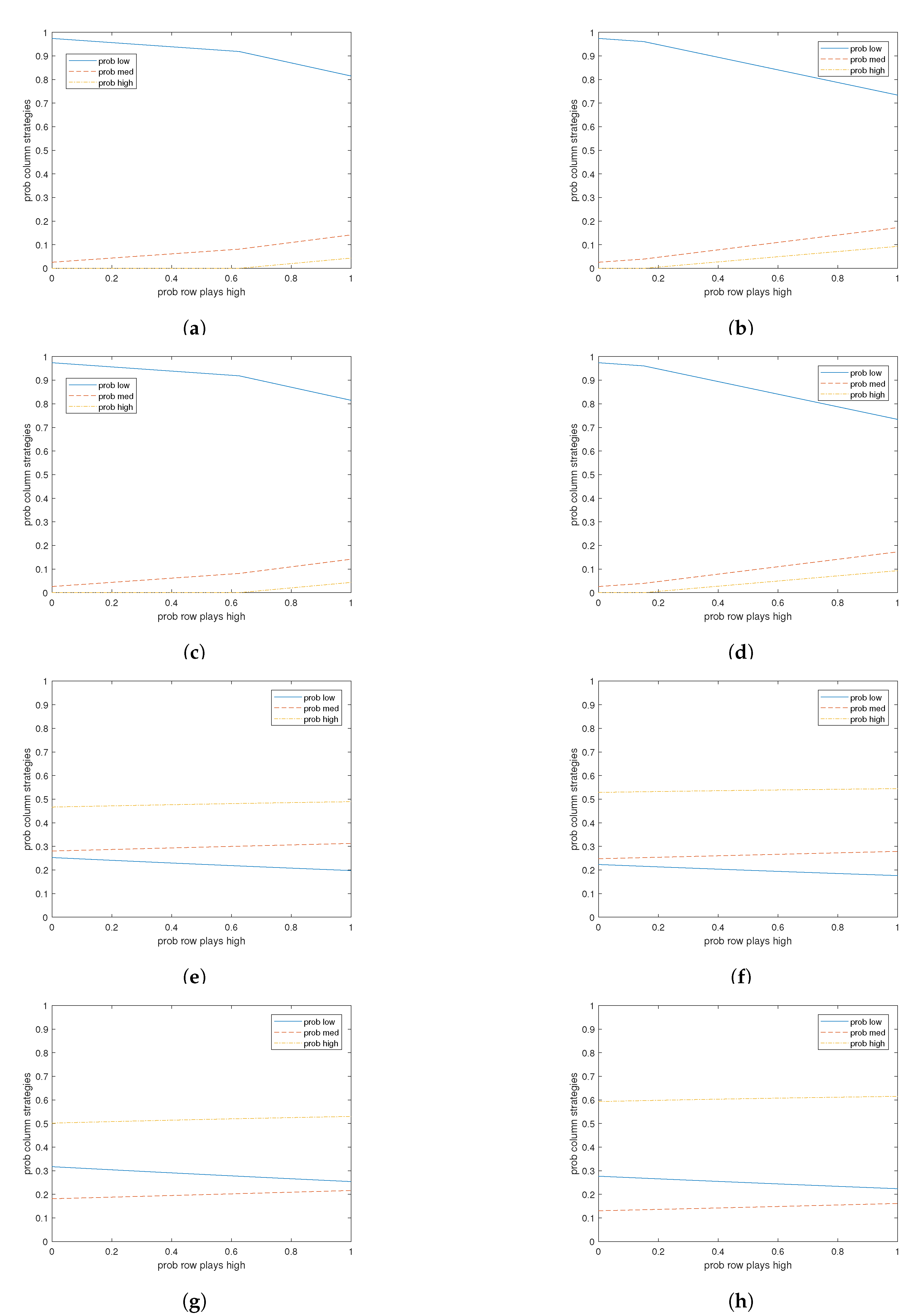
We consider when the row player is an expected utility maximizer and the column player is a perturbed utility player. We plot the best response probabilities for the column player in Figure 1, for four types of perturbation functions and two values of payoffs. Specific details on payoffs and perturbation functions are detailed in the code, available on the authors’ websites.

The left column corresponds to low payoffs for the high action of the column player and the right column corresponds to higher payoffs. The top row of Figure 1 is a quadratic perturbation function. Importantly, it allows complementarity between the medium and high strategies as the payoff to the high action increases. Here, as payoffs to the high action increase, the probability of playing the high action as a best response increases as expected, but the probability of playing the medium action also increases, indicating complementarity.

The next three rows do not allow complementarity. Figure 1c,d in the second row correspond to (quadratic) control costs, Figure 1e,f are logit perturbations, and Figure 1g,h are nested logit perturbations.

In this paper, we focus on best responses because a detailed theoretical analysis of equilibrium is beyond the scope of the paper. With that said, a simple equilibrium analysis is possible by supposing the row player has the high action as a dominant strategy. Then complementarity shows up for equilibrium comparative statics in Figure 1a,b by analogous reasoning as before. Specifically, the payoff of the high action increased, and both the medium and high probabilities increased in response.

6. Discussion

This paper shows existence of Nash equilibria in concave perturbed utility games, relates the approach to quantal response equilibria, develops the nested logit equilibrium, and introduces quadratic perturbed utility games. Thus, we link the literature on Nash equilibrium without expected utility which has not been used in applications to quantal response equilibrium (QRE) that has been extensively used in applications. We also provide the reader with several classes of perturbations that allow flexibility in best responses and can be used in the study of games. Other perturbations that may be useful are developed for discrete choice analysis in [9,10]. Although many of the models presented have many parameters, one can simplify estimation by making homogeneity assumptions across individuals.9 By presenting a tractable class of games, we hope this paper is able to re-introduce games of non-expected utility preferences to those unfamiliar with the earlier work in [22,23] in light of the new experimental evidence that supports a preference for randomization.

References

1. McKelvey, R.D.; Palfrey, T.R. Quantal response equilibria for normal form games. Games Econ. Behav. 1995, 10, 6–38. [Google Scholar] [CrossRef]
2. McKelvey, R.D.; Palfrey, T.R. Quantal response equilibria for extensive form games. Exp. Econ. 1998, 1, 41. [Google Scholar] [CrossRef]
3. Hofbauer, J.; Sandholm, W.H. On the global convergence of stochastic fictitious play. Econometrica 2002, 70, 2265–2294. [Google Scholar] [CrossRef]
4. Allen, R.; Rehbeck, J. Identification with additively separable heterogeneity. Econometrica 2019, 87, 1021–1054. [Google Scholar] [CrossRef]
5. Melo, E.; Pogorelskiy, K.; Shum, M. Testing the quantal response hypothesis. Int. Econ. Rev. 2019, 60, 53–74. [Google Scholar] [CrossRef]
6. van Damme, E. Refining the Equilibrium Concept for Bimatrix Games via Control Costs; Memorandum COSOR 82-02; Eindhoven University of Technology: Eindhoven, The Netherlands, 1981. [Google Scholar]
7. van Damme, E. Control costs. In Stability and Perfection of Nash Equilibria; Springer: Berlin/Heidelberg, Germany, 1987; pp. 62–77. [Google Scholar]
8. Debreu, G. A social equilibrium existence theorem. Proc. Natl. Acad. Sci. USA 1952, 38, 886–893. [Google Scholar] [CrossRef] [Green Version]
9. Fosgerau, M.; Monardo, J.; Palma, A.D. The Inverse Product Differentiation Logit Model. Available online: http://dx.doi.org/10.2139/ssrn.31410412019 (accessed on 29 December 2020).
10. Monardo, J. The Flexible Inverse Logit (Fil) Model. Available online: http://dx.doi.org/10.2139/ssrn.3388972 (accessed on 29 December 2020).
11. Rosenthal, R.W. A bounded-rationality approach to the study of noncooperative games. Int. J. Game Theory 1989, 18, 272–292. [Google Scholar] [CrossRef]
12. Voorneveld, M. Probabilistic choice in games: Properties of Rosenthal’s t-solutions. Int. J. Game Theory 2006, 34, 105–121. [Google Scholar] [CrossRef] [Green Version]
13. Stahl, D.O. Entropy control costs and entropic equilibria. Int. J. Game Theory 1990, 19, 129–138. [Google Scholar] [CrossRef]
14. Mattsson, L.; Weibull, J.W. Probabilistic choice and procedurally bounded rationality. Games Econ. Behav. 2002, 41, 61–78. [Google Scholar] [CrossRef]
15. Goeree, J.K.; Holt, C.A.; Palfrey, T.R. Regular quantal response equilibrium. Exp. Econ. 2005, 8, 347–367. [Google Scholar] [CrossRef] [Green Version]
16. Goeree, J.K.; Holt, C.A.; Palfrey, T.R. Quantal Response Equilibrium: A Stochastic Theory of Games; Princeton University Press: Princeton, NJ, USA, 2016. [Google Scholar]
17. Selten, R. Reexamination of the perfectness concept for equilibrium points in extensive games. Int. J. Game Theory 1975, 4, 25–55. [Google Scholar] [CrossRef] [Green Version]
18. Melo, E. On the Uniqueness of Quantal Response Equilibria. Available online: http://dx.doi.org/10.2139/ssrn.3631575 (accessed on 29 December 2020).
19. Machina, M.J. Expected utility analysis without the independence axiom. Econom. J. Econom. Soc. 1982, 50, 277–323. [Google Scholar] [CrossRef] [Green Version]
20. Nash, J. Non-cooperative games. Ann. Math. 1951, 54, 286–295. [Google Scholar] [CrossRef]
21. Neumann, J.V.; Morgenstern, O. Theory of Games and Economic Behavior; Princeton University Press: Princeton, NJ, USA, 1953. [Google Scholar]
22. Crawford, V.P. Equilibrium without independence. J. Econ. Theory 1990, 50, 127–154. [Google Scholar] [CrossRef] [Green Version]
23. Dekel, E.; Safra, Z.; Segal, U. Existence and dynamic consistency of nash equilibrium with non-expected utility preferences. J. Econ. Theory 1991, 55, 229–246. [Google Scholar] [CrossRef]
24. Machina, M.J. Stochastic choice functions generated from deterministic preferences over lotteries. Econ. J. 1985, 95, 575–594. [Google Scholar] [CrossRef]
25. McFadden, D.L.; Fosgerau, M. A Theory of the Perturbed Consumer with General Budgets; Technical Report; National Bureau of Economic Research: Cambridge, MA, USA, 2012. [Google Scholar]
26. Fudenberg, D.; Iijima, R.; Strzalecki, T. Stochastic choice and revealed perturbed utility. Econometrica 2015, 83, 2371–2409. [Google Scholar] [CrossRef] [Green Version]
27. Allen, R.; Rehbeck, J. Revealed Stochastic Choice with Attributes (25 January 2019). Available online: https://ssrn.com/abstract=2818041 (accessed on 29 December 2020).
28. Iijima, R. Deterministic Equilibrium Selection under Payoff-Perturbed Dynamics. Available online: http://dx.doi.org/10.2139/ssrn.2462656 (accessed on 29 December 2020).
29. Allen, R.; Rehbeck, J. Hicksian complementarity and perturbed utility models. Econ. Theory Bull. 2019, 8, 245–261. [Google Scholar] [CrossRef]
30. Ma, W. Perturbed utility and general equilibrium analysis. J. Math. Econ. 2017, 73, 122–131. [Google Scholar] [CrossRef] [Green Version]
31. Karni, E.; Safra, Z. Ascending bid auctions with behaviorally consistent bidders. Ann. Oper. Res. 1989, 19, 435–446. [Google Scholar] [CrossRef]
32. Machina, M.J. Dynamic consistency and non-expected utility models of choice under uncertainty. J. Econ. Lit. 1989, 27, 1622–1668. [Google Scholar]
33. Segal, U. Two-stage lotteries without the reduction axiom. Econometrica 1990, 58, 349–377. [Google Scholar] [CrossRef] [Green Version]
34. Mosteller, F.; Nogee, P. An experimental measurement of utility. J. Political Econ. 1951, 59, 371–404. [Google Scholar] [CrossRef]
35. Sopher, B.; Narramore, J.M. Stochastic choice and consistency in decision making under risk: An experimental study. Theory Decis. 2000, 48, 323–350. [Google Scholar] [CrossRef]
36. Agranov, M.; Ortoleva, P. Stochastic choice and preferences for randomization. J. Political Econ. 2017, 125, 40–68. [Google Scholar] [CrossRef] [Green Version]
37. Dwenger, N.; Kübler, D.; Weizsäcker, G. Flipping a coin: Evidence from university applications. J. Public Econ. 2018, 167, 240–250. [Google Scholar] [CrossRef] [Green Version]
38. Burghart, D.R. The two faces of independence: Betweenness and homotheticity. Theory Decis. 2019, 88, 567–593. [Google Scholar] [CrossRef] [Green Version]
39. Feldman, P.; Rehbeck, J. Revealing a Preference for Mixing: An Experimental Study of Risk. Technical Report. 2020. Available online: https://econweb.ucsd.edu/~pfeldman/pdfs/Preferences%20over%20Lotteries_v10.pdf (accessed on 29 December 2020).
40. Agranov, M.; Ortoleva, P. Ranges of Preferences and Randomization. Technical Report. 2020. Available online: https://agranov.caltech.edu/documents/13172/Ranges_5.pdf (accessed on 29 December 2020).
41. Agranov, M.; Healy, P.J.; Nielsen, K. Stable Randomization. Available online: http://dx.doi.org/10.2139/ssrn.3544929 (accessed on 29 December 2020).
42. Luce, R.D.; Raiffa, H. Games and Decisions: Introduction and Critical Survey; Courier Corporation: North Chelmsford, MA, USA, 1989. [Google Scholar]
43. Bresnahan, T.F.; Reiss, P.C. Entry in monopoly market. Rev. Econ. Stud. 1990, 57, 531–553. [Google Scholar] [CrossRef]
44. Tamer, E. Incomplete simultaneous discrete response model with multiple equilibria. Rev. Econ. Stud. 2003, 70, 147–165. [Google Scholar] [CrossRef]
45. Chambers, C.P.; Cuhadaroglu, T.; Masatlioglu, Y. Behavioral Influence. Technical Report. 2019. Available online: http://econweb.umd.edu/~masatlioglu/Influence_Conformity.pdf (accessed on 29 December 2020).
46. Kahneman, D.; Tversky, A. Prospect theory: An analysis of decision under risk. Econometrica 1979, 47, 263–292. [Google Scholar] [CrossRef] [Green Version]
47. Quiggin, J. A theory of anticipated utility. J. Econ. Behav. Organ. 1982, 3, 323–343. [Google Scholar] [CrossRef]
48. Becker, R.A.; Chakrabarti, S.K. Satisficing behavior, brouwer’s fixed point theorem and nash equilibrium. Econ. Theory 2005, 26, 63–83. [Google Scholar] [CrossRef]
49. Cominetti, R.; Melo, E.; Sorin, S. A payoff-based learning procedure and its application to traffic games. Games Econ. Behav. 2010, 70, 71–78. [Google Scholar] [CrossRef]
50. Anderson, S.P.; Palma, A.D.; Thisse, J. Discrete Choice Theory of Product Differentiation; MIT Press: Cambridge, MA, USA, 1992. [Google Scholar]
51. Sims, C.A. Implications of rational inattention. J. Monet. Econ. 2003, 50, 665–690. [Google Scholar] [CrossRef] [Green Version]
52. Matejka, F.; McKay, A. Rational inattention to discrete choices: A new foundation for the multinomial logit model. Am. Econ. Rev. 2014, 105, 272–298. [Google Scholar] [CrossRef] [Green Version]
53. Jiang, G.; Fosgerau, M.; Lo, H.K. Route choice, travel time variability, and rational inattention. Transp. Res. Part Methodol. 2020, 132, 188–207. [Google Scholar] [CrossRef]
54. Train, K.E. Discrete Choice Methods with Simulation; Cambridge University Press: Cambridge, UK, 2009. [Google Scholar]
55. Kovach, M.; Tserenjigmid, G. Behavioral Foundations of Nested Stochastic Choice and Nested Logit. Available online: http://dx.doi.org/10.2139/ssrn.3437165 (accessed on 29 December 2020).
1.
This can be deduced from the single agent aggregation results of Hofbauer and Sandholm [3] or Allen and Rehbeck [4] (see also [5]).
2.
Professor van Damme in fact says the idea originates even earlier from discussions with Professor Selten.
3.
Goeree et al. [16] also linked the development of QRE to games with decision errors that dates back to the work by Selten [17].
4.
Perturbed utility preferences are tractable and have been studied general for individual stochastic choice [25,26,27], population games [28], consumer choice [25,29], and general equilibrium [30].
5.
We do not concern ourselves with issues of dynamic consistency as studied in [23]. An interested reader can follow the discussion in [31,32,33], and the following literature.
6.
One could also use the fixed point theorem in [48] to develop a constructive function that updates a given set of choices to a fixed point.
7.
For a behavioral characterization of nested logit discrete choice with menu variation, see [55].
8.
We also mention that even when η n , > 0 but not in [0,1] the best response function conditional on p n is a singleton as shown by Allen and Rehbeck [27] so a Nash equilibrium exists by Debreu [8]. When η n , > 1 , this allows complementarity following Allen and Rehbeck [29] within a nest and cannot be imitated by any additive random error used to generate quantal response equilibria.
9.
For example, letting α n , j = α for each individual and strategy in Equation (1) creates a one-parameter model when U n , j and d n , j are pre-specified.
Figure 1. Best responses of the column player for a low payoff of the high action (left) and a higher payoff of the high action (right): (a,b) quadratic perturbations; (c,d) control perturbations; (e,f) logit perturbations; and (g,h) nested logit perturbations.
Games 12 00020 g001