A Two-Period Game Theoretic Model of Zero-Day Attacks with Stockpiling


Abstract
1. Introduction
1.1. Background
1.2. Contribution
1.3. Literature
1.3.1. Game Theoretic Analyses
1.3.2. Detection, Prioritization, Ranking, and Classification
1.3.3. Detection and Identification by Applying Probability Theory and Statistics
1.3.4. Detection Applying Learning
1.3.5. Mitigation, Robustness, Recovery, and Simulation
1.3.6. Filtering, Protocol Context, Honeypots, and Signatures
1.3.7. Cyber Security
1.3.8. Information Security
1.4. Article Organization
2. The Model
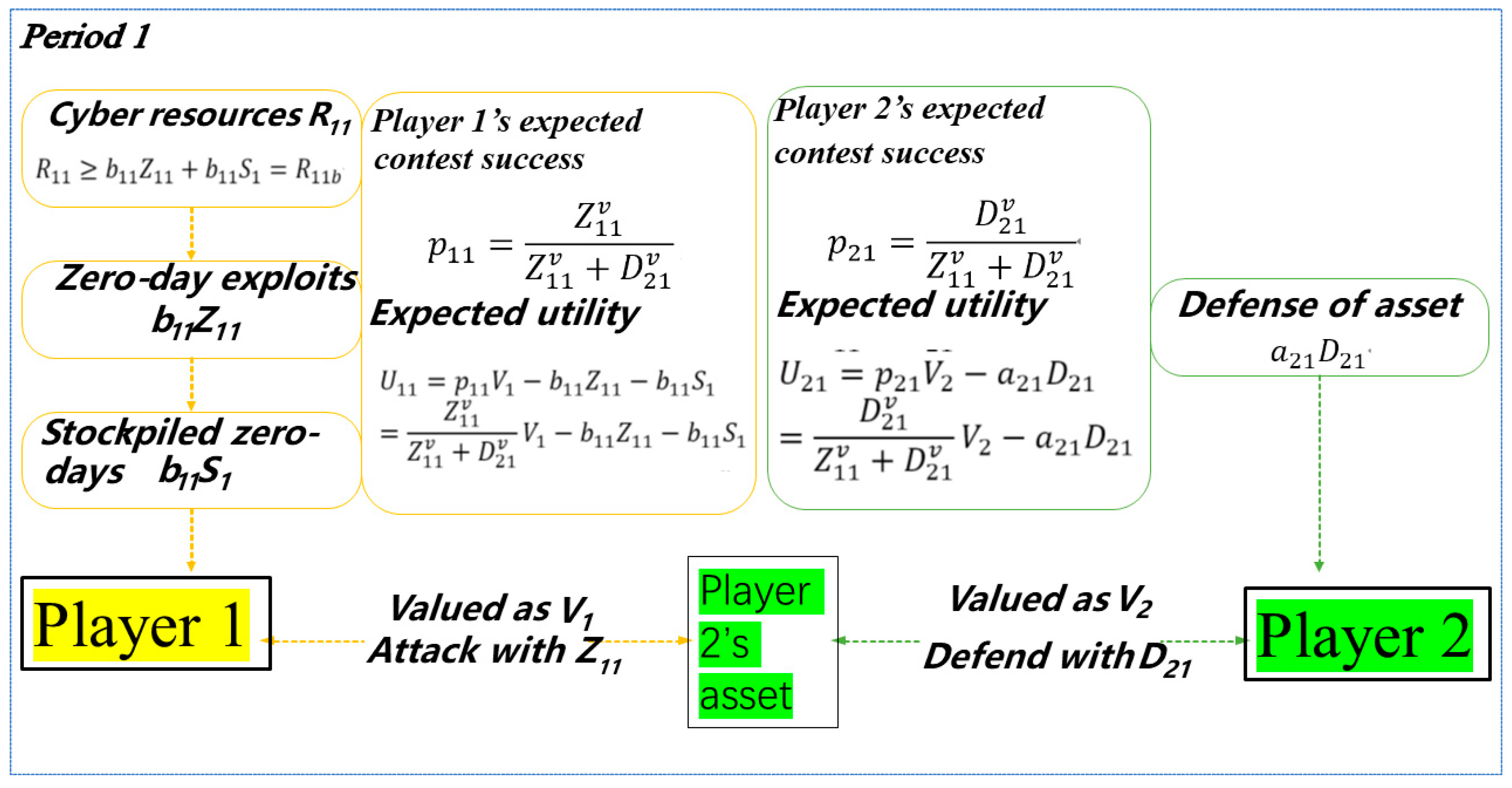
2.1. Period 1
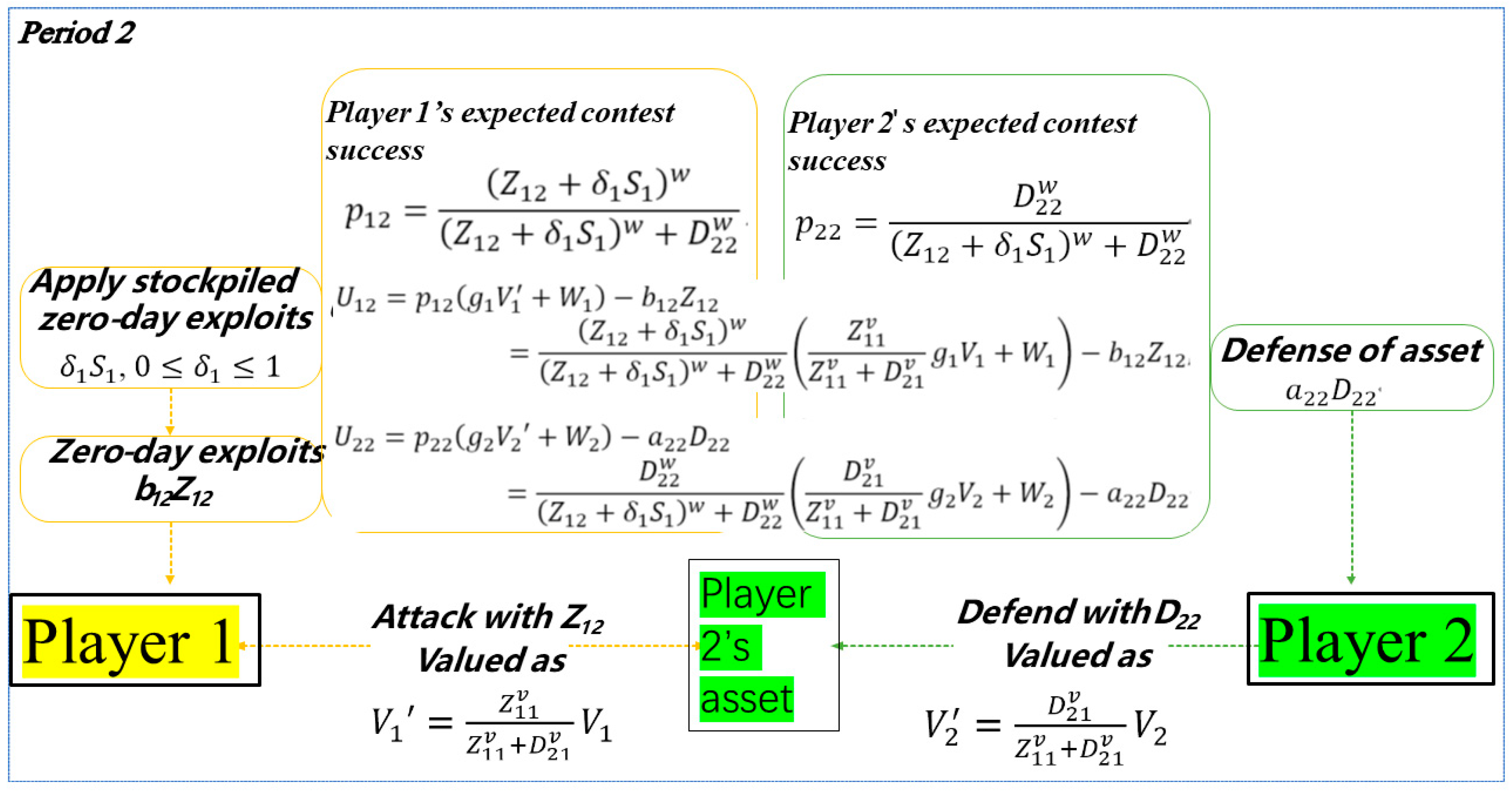
2.2. Period 2
3. Solving the Model
3.1. Solutions 1, 2, 3 (, , )
3.1.1. Solving Period 2
3.1.2. Solving Period 1
3.1.3. Solution 3 ()
3.2. Solutions 4–8 (, , )
3.2.1. Solution 4 (, )
3.2.2. Solution 5 (, )
3.2.3. Solutions 6–8 (, , )
3.3. Solution 9 ()
3.4. Solution 10 (, )
3.5. Solution 11 ()
4. Illustrating the Solution
5. Discussion
6. Conclusions
Author Contributions
Funding
Acknowledgments
Conflicts of Interest
Nomenclature
| Parameters | |
| Player s cyber resources in Period 1, | |
| Player 2′s unit effort cost of defense in Period , , | |
| Player 1′s unit effort cost of developing zero-day capabilities in Period , , | |
| Player ’s valuation of Player 2′s asset, | |
| Growth factor of asset from Period 1 to Period 2, | |
| Player ’s valuation of Player 2′s asset acquired in Period 2, | |
| Contest intensity in Period 1, | |
| Contest intensity in Period 2, | |
| Player 1′s zero-day appreciation factor of stockpiled zero-day exploits from Period 1 to Period 2, | |
| Player ’s time discount factor, | |
| Strategic Choice Variables | |
| Player 1′s effort to develop zero-day capabilities in Period 1, | |
| Player 2′s defense effort in Period 1, | |
| Player 1′s effort to develop zero-day capabilities in Period 2, | |
| Player 2′s defense effort in Period 2, | |
| Dependent Variables | |
| Player 1′s stockpiling of zero-day exploits in Period 1 for use in Period 2, | |
| Player ’s expected contest success in Period , , | |
| Player ’s expected utility in Period , | |
| Player ’s expected utility over both time periods, | |
| The actual amount of resources used by Player 1 in Period 1 | |
References
- Nakashima, E.; Warrick, J. Stuxnet Was Work of U.S. and Israeli Experts, Officials Say. 2012. Available online: https://cyber-peace.org/wp-content/uploads/2013/06/Stuxnet-was-work-of-U.S.pdf (accessed on 16 December 2020).
- Cherepanov, A. Windows Zero-Day CVE-2019-1132 Exploited in Targeted Attacks. 2019. Available online: https://www.welivesecurity.com/2019/07/10/windows-zero-day-cve-2019-1132-exploit/ (accessed on 14 December 2020).
- PhishProtection. Recent Zero-Day Attacks: Top Examples and How to Prevent It. 2020. Available online: https://www.phishprotection.com/content/zero-day-protection/recent-zero-day-attacks/ (accessed on 14 December 2020).
- Hausken, K.; Welburn, J.W. Attack and Defense Strategies in Cyber War Involving Production and Stockpiling of Zero-Day Cyber Exploits. Inf. Syst. Front. 2020, 1–12. [Google Scholar] [CrossRef]
- Chen, H.; Han, Q.; Jajodia, S.; Lindelauf, R.; Subrahmanian, V.S.; Xiong, Y. Disclose or Exploit? A Game-Theoretic Approach to Strategic Decision Making in Cyber-Warfare. IEEE Syst. J. 2020, 14, 3779–3790. [Google Scholar] [CrossRef]
- Ablon, L.; Bogart, A. Zero Days, Thousands of Nights: The Life and Times of Zero-Day Vulnerabilities and Their Exploits; RAND Corporation: Santa Monica, CA, USA, 2017. [Google Scholar]
- Singh, U.K.; Joshi, C.; Kanellopoulos, D. A Framework for Zero-Day Vulnerabilities Detection and Prioritization. J. Inf. Secur. Appl. 2019, 46, 164–172. [Google Scholar] [CrossRef]
- Al-Rimy, B.A.S.; Maarof, M.A.; Prasetyo, Y.A.; Shaid, S.Z.M.; Ariffin, A.F.M.; Malaysia, S.K.C. Zero-Day Aware Decision Fusion-Based Model for Crypto-Ransomware Early Detection. Int. J. Integr. Eng. 2018, 10, 82–88. [Google Scholar] [CrossRef]
- Venkatraman, S.; Alazab, M. Use of Data Visualisation for Zero-Day Malware Detection. Secur. Commun. Netw. 2018, 2018, 1–13. [Google Scholar] [CrossRef]
- Sun, X.y.; Dai, J.; Liu, P.; Singhal, A.; Yen, J. Using Bayesian Networks for Probabilistic Identification of Zero-Day Attack Paths. IEEE Trans. Inf. Forensics Secur. 2018, 13, 2506–2521. [Google Scholar] [CrossRef]
- Parrend, P.; Navarro, J.; Guigou, F.; Deruyver, A.; Collet, P. Foundations and Applications of Artificial Intelligence for Zero-Day and Multi-Step Attack Detection. EURASIP J. Inf. Secur. 2018, 2018, 4. [Google Scholar] [CrossRef]
- Singh, S.; Sharma, P.K.; Moon, S.Y.; Park, J.H. A Hybrid Layered Architecture for Detection and Analysis of Network Based Zero-Day Attack. Comput. Commun. 2017, 106, 100–106. [Google Scholar] [CrossRef]
- Kim, J.Y.; Bu, S.J.; Cho, S.B. Zero-Day Malware Detection Using Transferred Generative Adversarial Networks Based on Deep Autoencoders. Inf. Sci. 2018, 460, 83–102. [Google Scholar] [CrossRef]
- Gupta, D.; Rani, R. Big Data Framework for Zero-Day Malware Detection. Cybern. Syst. 2018, 49, 103–121. [Google Scholar] [CrossRef]
- Sharma, V.; Lee, K.; Kwon, S.; Kim, J.; Park, H.; Yim, K.; Lee, S.Y. A Consensus Framework for Reliability and Mitigation of Zero-Day Attacks in IoT. Secur. Commun. Networks 2017, 2017, 1–24. [Google Scholar] [CrossRef]
- Haider, W.; Creech, G.; Xie, Y.; Hu, J.K. Windows Based Data Sets for Evaluation of Robustness of Host Based Intrusion Detection Systems (IDS) to Zero-Day and Stealth Attacks. Future Internet 2016, 8, 29. [Google Scholar] [CrossRef]
- Tran, H.; Campos-Nanez, E.; Fomin, P.; Wasek, J. Cyber Resilience Recovery Model to Combat Zero-Day Malware Attacks. Comput. Secur. 2016, 61, 19–31. [Google Scholar] [CrossRef]
- Tidy, L.; Woodhead, S.; Wetherall, J. Simulation of Zero-Day Worm Epidemiology in the Dynamic, Heterogeneous Internet. J. Def. Model. Simul. Appl. Methodol. Technol. 2015, 12, 123–138. [Google Scholar] [CrossRef]
- Chowdhury, M.U.; Abawajy, J.H.; Kelarev, A.V.; Hochin, T. Multilayer Hybrid Strategy for Phishing Email Zero-Day Filtering. Concurr. Comput. Pract. Exp. 2017, 29, e3929. [Google Scholar] [CrossRef]
- Duessel, P.; Gehl, C.; Flegel, U.; Dietrich, S.; Meier, M. Detecting Zero-Day Attacks Using Context-Aware Anomaly Detection at the Application-Layer. Int. J. Inf. Secur. 2017, 16, 475–490. [Google Scholar] [CrossRef]
- Chamotra, S.; Sehgal, R.K.; Misra, R.S. Honeypot Baselining for Zero Day Attack Detection. Int. J. Inf. Secur. Priv. 2017, 11, 63–74. [Google Scholar] [CrossRef]
- Afek, Y.; Bremler-Barr, A.; Feibish, S.L. Zero-Day Signature Extraction for High-Volume Attacks. IEEE/ACM Trans. Netw. 2019, 27, 691–706. [Google Scholar] [CrossRef]
- Baliga, S.; De Mesquita, E.B.; Wolitzky, A. Deterrence with Imperfect Attribution. Am. Political Sci. Rev. 2020, 114, 1155–1178. [Google Scholar] [CrossRef]
- Edwards, B.; Furnas, A.; Forrest, S.; Axelrod, R. Strategic aspects of cyberattack, attribution, and blame. Proc. Natl. Acad. Sci. USA 2017, 114, 2825–2830. [Google Scholar] [CrossRef] [PubMed]
- Welburn, J.W.; Grana, J.; Schwindt, K. Cyber Deterrence or: How We Learned to Stop Worrying and Love the Signal; RAND Corporation: Santa Monica, CA, USA, 2019. [Google Scholar]
- Nagurney, A.; Shukla, S. Multifirm models of cybersecurity investment competition vs. cooperation and network vulnerability. Eur. J. Oper. Res. 2017, 260, 588–600. [Google Scholar] [CrossRef]
- Levitin, G.; Hausken, K.; Taboada, H.A.; Coit, D.W. Data Survivability vs. Security in Information Systems. Reliab. Eng. Syst. Saf. 2012, 100, 19–27. [Google Scholar] [CrossRef]
- Enders, W.; Sandler, T. What Do We Know About the Substitution Effect in Transnational Terrorism? In Researching Terrorism: Trends, Achievements, Failures; Silke, A., Ilardi, G., Eds.; Frank Cass: Ilfords, UK, 2003. [Google Scholar]
- Hausken, K. Income, Interdependence, and Substitution Effects Affecting Incentives for Security Investment. J. Account. Public Policy 2006, 25, 629–665. [Google Scholar] [CrossRef]
- Lakdawalla, D.N.; Zanjani, G. Insurance, Self-Protection, and the Economics of Terrorism. J. Public Econ. 2005, 89, 1891–1905. [Google Scholar]
- Hausken, K. Returns to Information Security Investment: The Effect of Alternative Information Security Breach Functions on Optimal Investment and Sensitivity to Vulnerability. Inf. Syst. Front. 2006, 8, 338–349. [Google Scholar] [CrossRef]
- Hausken, K. Returns to Information Security Investment: Endogenizing the Expected Loss. Inf. Syst. Front. 2014, 16, 329–336. [Google Scholar] [CrossRef]
- Hausken, K. Information Sharing Among Firms and Cyber Attacks. J. Account. Public Policy 2007, 26, 639–688. [Google Scholar] [CrossRef]
- Hausken, K. A Strategic Analysis of Information Sharing Among Cyber Attackers. J. Inf. Syst. Technol. Manag. 2015, 12, 245–270. [Google Scholar] [CrossRef]
- Hausken, K. Information Sharing Among Cyber Hackers in Successive Attacks. Int. Game Theory Rev. 2017, 19, 33. [Google Scholar] [CrossRef]
- Hausken, K. Security Investment, Hacking, and Information Sharing between Firms and between Hackers. Games 2017, 8, 23. [Google Scholar] [CrossRef]
- Hausken, K. Proactivity and Retroactivity of Firms and Information Sharing of Hackers. Int. Game Theory Rev. 2018, 20, 1750030. [Google Scholar] [CrossRef]
- Do, C.T.; Tran, N.H.; Hong, C.; Kamhoua, C.A.; Kwiat, K.A.; Blasch, E.; Ren, S.; Pissinou, N.; Iyengar, S.S. Game theory for cyber security and privacy. ACM Comput. Surv. 2017, 50, 1–37. [Google Scholar] [CrossRef]
- Hausken, K.; Levitin, G. Review of Systems Defense and Attack Models. Int. J. Perform. Eng. 2012, 8, 355–366. [Google Scholar] [CrossRef]
- Roy, S.; Ellis, C.; Shiva, S.; Dasgupta, D.; Shandilya, V.; Wu, Q. A survey of game theory as applied to network security. In Proceedings of the 2010 43rd Hawaii International Conference on System Sciences, Honolulu, HI, USA, 5–8 January 2010; pp. 1–10. [Google Scholar]
- Tullock, G. Efficient Rent-Seeking. In Toward a Theory of the Rent-Seeking Society; Buchanan, J.M., Tollison, R.D., Tullock, G., Eds.; Texas A&M University Press: College Station, TX, USA, 1980; pp. 97–112. [Google Scholar]
- Hausken, K.; Levitin, G. Efficiency of Even Separation of Parallel Elements with Variable Contest Intensity. Risk Anal. 2008, 28, 1477–1486. [Google Scholar] [CrossRef] [PubMed]
- Hausken, K. Additive Multi-Effort Contests. Theory Decis. 2020, 89, 203–248. [Google Scholar] [CrossRef]
- Congleton, R.D.; Hillman, A.L.; Konrad, K.A. 40 Years of Research on Rent Seeking—Applications: Rent Seeking in Practice; Springer: Berlin/Heidelberg, Germany, 2008; Volume 2. [Google Scholar]


| Sol. Stockpiling | Budget Constraint | Period 2 | Description | Section | |
|---|---|---|---|---|---|
| 1 | , | Player 1 neither stockpiles nor utilizes entire budget | Section 3.1.2 | ||
| 2 | , | Player 1 stockpiles and utilizes entire budget | Section 3.1.2 | ||
| 3 | , | Player 1 does not stockpile and utilizes entire budget | Section 3.1.3 | ||
| 4 | Player 2 is deterred; Player 1 is superior | Section 3.2.1 | |||
| 5 | Player 2 is deterred; Player 1 utilizes entire budget | Section 3.2.2 | |||
| 6 | , | , Player 2 is not deterred | Section 3.2.3 | ||
| 7 | , | ,, Player 2 is not deterred | Section 3.2.3 | ||
| 8 | , | Player 2 is not deterred, though Player 1 is superior | Section 3.2.3 | ||
| 9 | , | Player 1 withdraws to ensure | Section 3.3 | ||
| 10 | , | Equally matched players; | Section 3.4 | ||
| 11 | Player 2 is deterred; Player 1 does not stockpile | Section 3.5 |
| Panel | Parameter(s) | Key Findings |
|---|---|---|
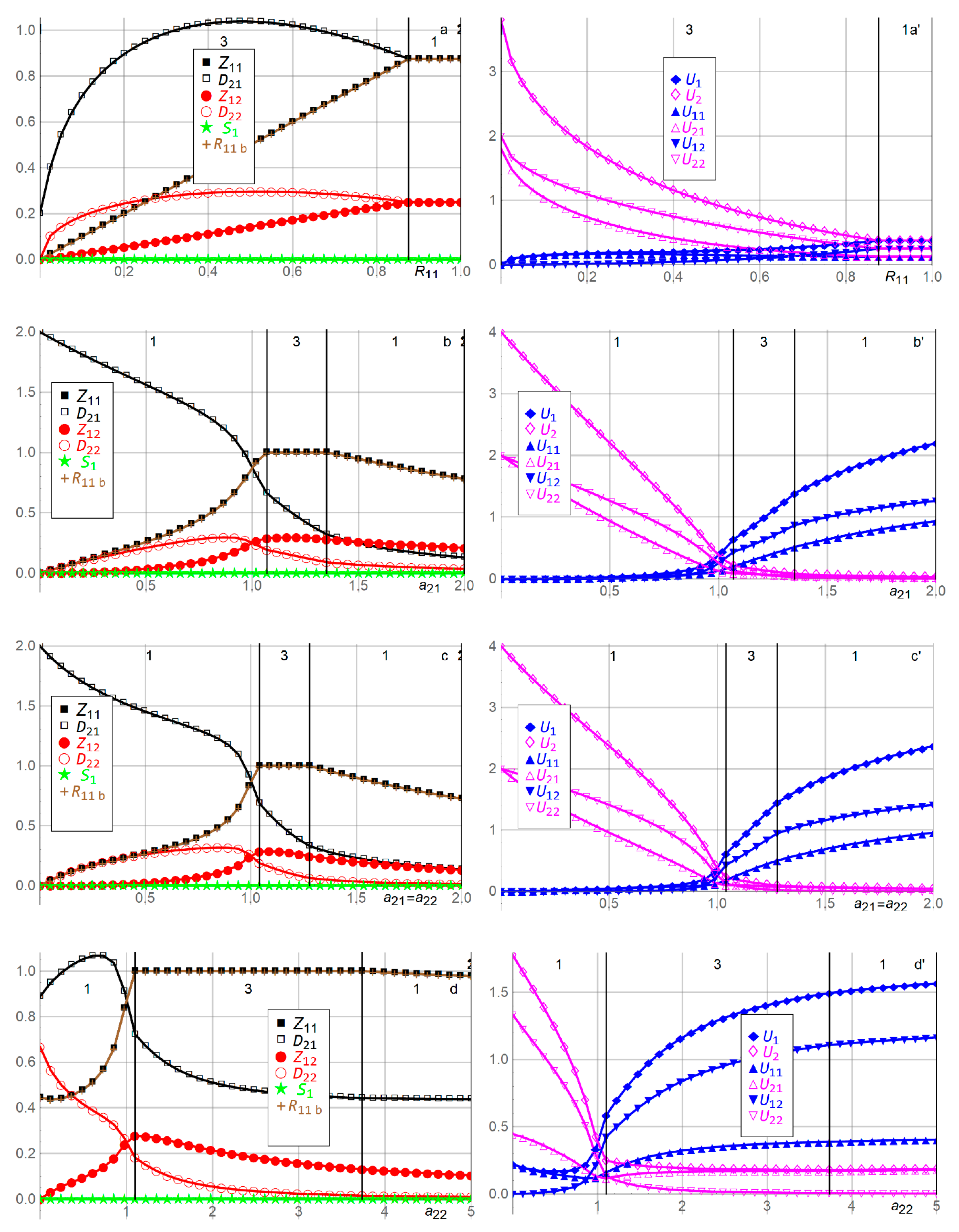
| a,a’ | As Player 1′s available resources in Period 1 decrease, its efforts in both periods decrease, while Player 2′s efforts in both periods are inverse U-shaped. Player 2 transitions from being inferior when Player 1 is resourceful to being competitive when the players are equally matched and being superior when Player 1 lacks resources. | |
| b,b’ | As Player 2′s unit effort cost of defense in Period 1 increases, its efforts decrease, while Player 1′s efforts are inverse U-shaped and resource-constrained. As decreases, Player 2′s Period 1 effort increases, while its Period 2 effort is inverse U-shaped, and Player 1′s efforts decrease. | |
| c,c’ | As Player 2′s unit defense costs in both periods increase (decrease), Player 2 becomes more disadvantaged (advantaged) than when only its unit effort cost of defense in Period 1 increases (decreases). | |
| d,d’ | If Player 2 can choose, it prefers being disadvantaged in Period 2 with high unit effort cost , when a less valuable asset is at stake, rather than being disadvantaged in the more important Period 1 with high unit effort cost . Similarly, Player 2 prefers being advantaged in the more important Period 1 with low unit effort cost , rather than being advantaged in Period 2 with high . | |
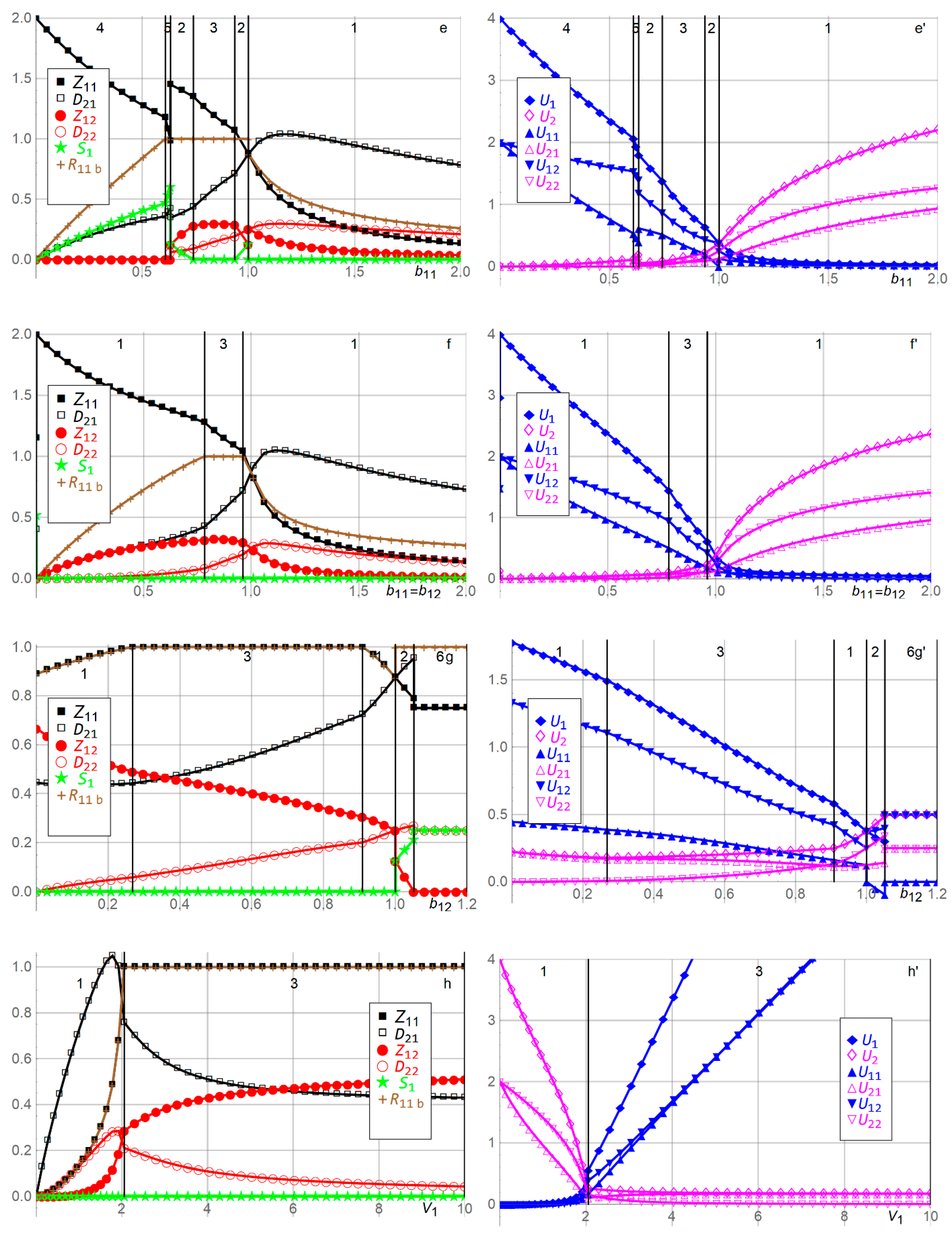
| e,e’ | Player 1 may stockpile when its unit effort cost of developing zero-day capabilities in Period 1 decreases, through three phases, below that of Period 2. First, Player 1 stockpiles as permitted by the budget and cuts back on the Period 2 effort. Second, Player 1 utilizes its entire budget in Period 1 without stockpiling, to exploit its advantage competitively over Player 2. Third, Player 1 eventually does not need to utilize its entire budget, attacks optimally in Period 1, and stockpiles sufficiently in Period 1 to deter Player 2 from defending in Period 2. | |
| f,f’ | As Player 1′s unit effort costs of developing zero-day capabilities increase equally in both periods, Player 1 does not stockpile and becomes more disadvantaged than when only one unit effort cost increases. As decrease, Player 1 becomes more advantaged than when only one unit effort cost decreases. | |
| g,g’ | As Player 1′s unit effort cost of developing zero-day capabilities in Period 2 increases above that of Period 1, Player 1 stockpiles more to exploit the advantage of the cheaper unit effort cost in Period 1, decreases the efforts in both periods, and accepts negative expected utility in Period 1 to ensure higher expected utility in Period 2. This continues until Player 1 can no longer afford to exert effort in Period 2. Player 1 instead focuses on Period 1 and stockpiles optimally for Period 2, as permitted by the budget constraint. | |
| h,h’ | As Player 1′s valuation of Player 2′s asset increases, Player 1 exerts higher efforts and eventually becomes resource-constrained, while Player 2 exerts lower efforts. As decreases, Player 1 exerts lower efforts and Player 2′s efforts are inverse U-shaped. | |
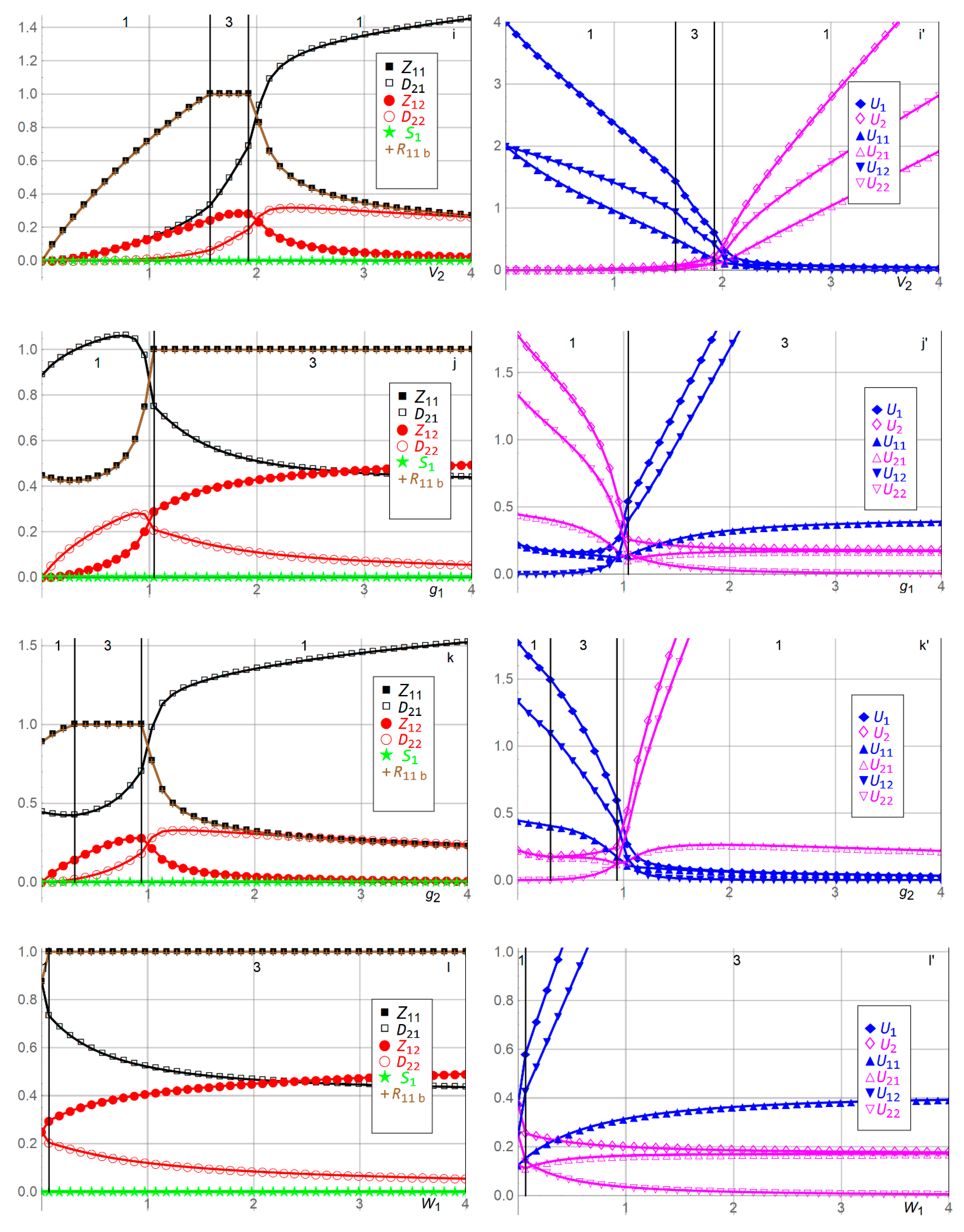
| i,i’ | As Player 2′s valuation of its own asset increases, Player 2 exerts concavely increasing Period 1 defense effort and inverse U-shaped Period 2 effort, while Player 1′s efforts decrease. As decreases, Player 2′s efforts decrease, while Player 1′s efforts are inverse U-shaped and resource-constrained. | |
| j,j’ | As Player 1′s growth factor of asset from Period 1 to Period 2 increases, Player 1′s efforts increase, subject to the resource constraint, while Player 2′s efforts decrease. As decreases, Player 1′s efforts decrease overall, while Player 2′s efforts are inverse U-shaped. | |
| k,k’ | As Player 2′s growth factor of asset from Period 1 to Period 2 increases, Player 2′s Period 1 effort increases, its Period 2 effort is inverse U-shaped, and Player 1′s efforts decrease. As decreases, Player 2′s efforts decrease overall, while Player 1′s efforts are inverse U-shaped and resource-constrained. | |
| l,l’ | As Player 1′s valuation of Player 2′s asset, acquired in Period 2, increases, Player 1′s efforts increase, subject to the budget constraint, while Player 2′s efforts decrease. | |
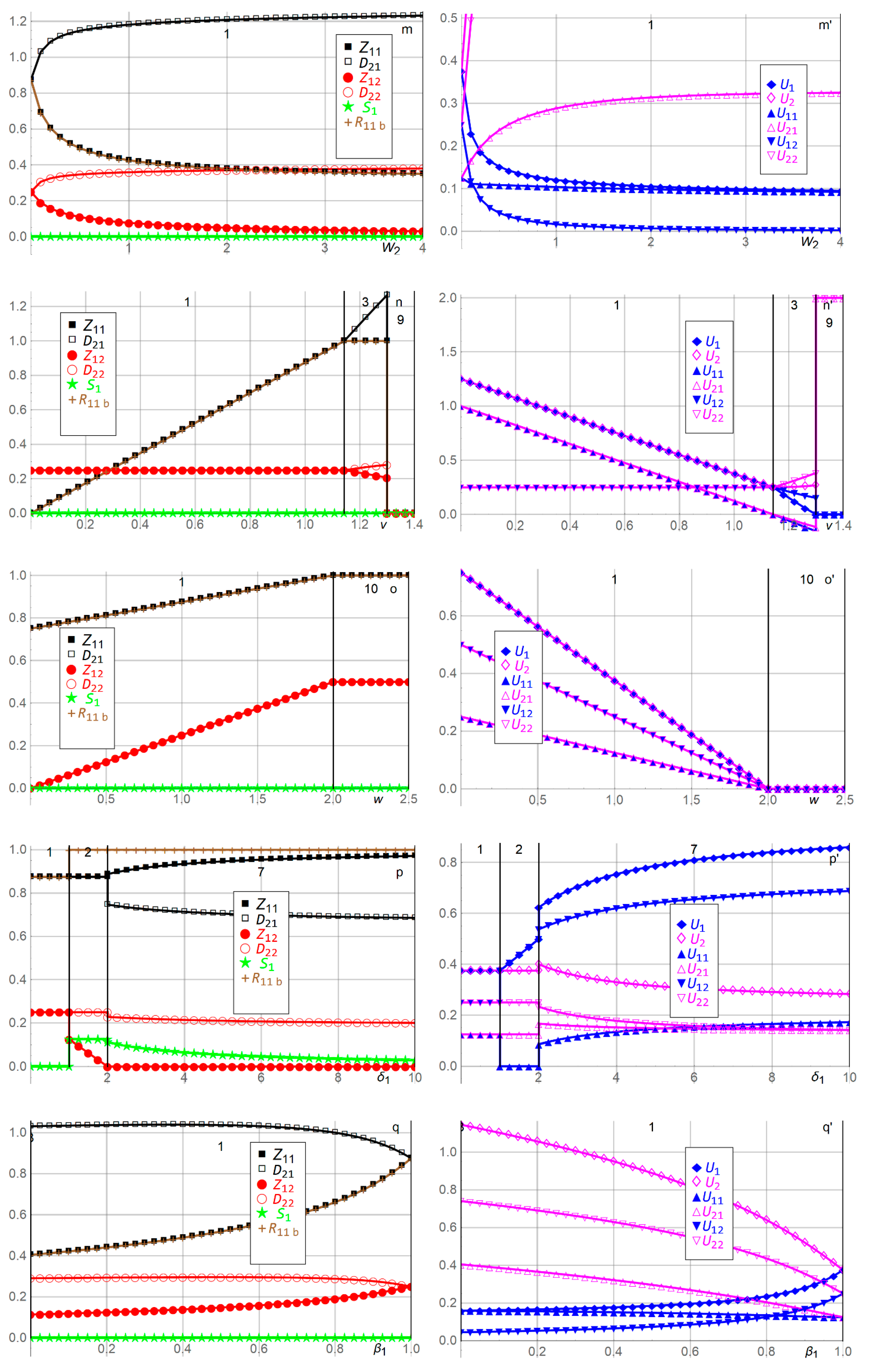
| m,m’ | As Player 2′s valuation of its own asset acquired in Period 2 increases, Player 2′s efforts increase concavely, while Player 1′s efforts decrease convexly. | |
| n,n’ | As the contest intensity in Period 1 increases, both players’ Period 1 efforts increase due to more fierce competition, until Player 1 reaches its budget constraint, after which Player 2 benefits. As decreases, both players’ Period 1 efforts decrease, causing higher expected utilities. | |
| o,o’ | As the contest intensity in Period 2 increases, both players’ efforts in both periods increase until the fiercer competition causes zero expected utilities to both players, assuming they are equally matched. | |
| p,p’ | As Player 1′s zero-day appreciation factor of stockpiled zero-day exploits from Period 1 to Period 2 increases above one, Player 1 immediately utilizes its entire Period 1 budget to attack and stockpile, cutting back on its Period 2 attack. This continues until Player 1′s stockpiling is so large that the Period 2 attack is no longer cost effective. Thereafter, Player 1 decreases its stockpiling (due to its appreciation) and increases its Period 1 attack, while Player 2 decreases its defense in both periods. | |
| q,q’ | As Player 1′s time discount factor decreases, so that Player 1 assigns less weight to the future Period 2, Player 1′s efforts decrease, causing lower expected utilities, while Player 2′s efforts increase overall, causing higher expected utilities. | |
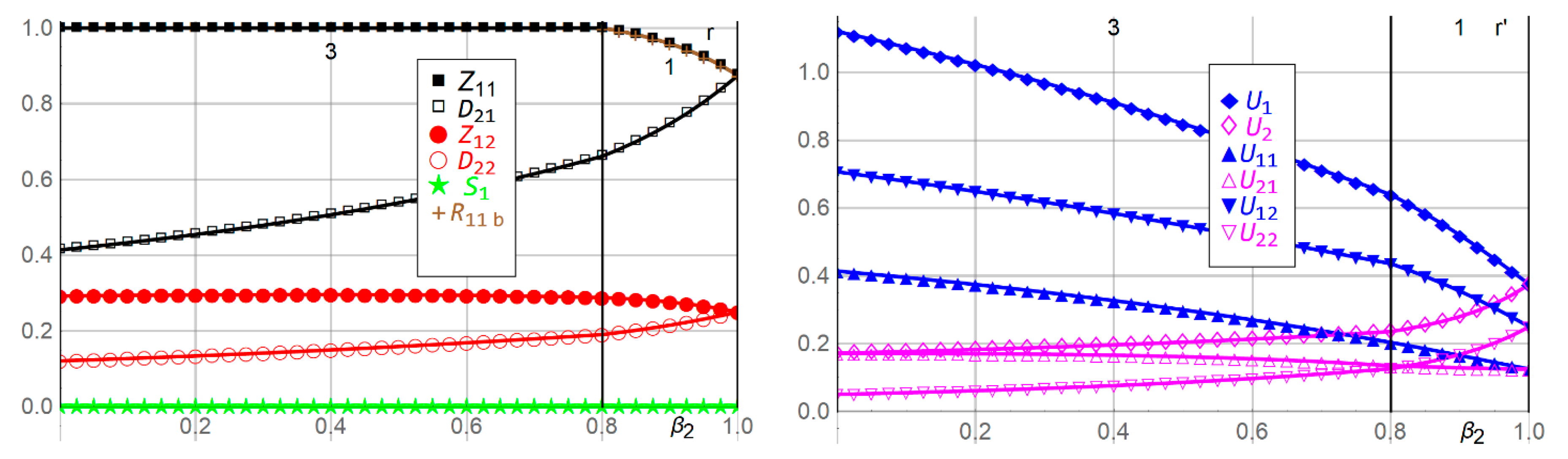
| r,r’ | As Player 2′s time discount factor decreases, so that Player 2 assigns less weight to the future Period 2, Player 2′s efforts decrease, causing lower expected utilities, while Player 1’s efforts increase, subject to the budget constraint, causing higher expected utilities. |
Publisher’s Note: MDPI stays neutral with regard to jurisdictional claims in published maps and institutional affiliations. |
© 2020 by the authors. Licensee MDPI, Basel, Switzerland. This article is an open access article distributed under the terms and conditions of the Creative Commons Attribution (CC BY) license (http://creativecommons.org/licenses/by/4.0/).
Share and Cite
Wang, G.; Welburn, J.W.; Hausken, K. A Two-Period Game Theoretic Model of Zero-Day Attacks with Stockpiling. Games 2020, 11, 64. https://doi.org/10.3390/g11040064
Wang G, Welburn JW, Hausken K. A Two-Period Game Theoretic Model of Zero-Day Attacks with Stockpiling. Games. 2020; 11(4):64. https://doi.org/10.3390/g11040064
Chicago/Turabian StyleWang, Guizhou, Jonathan W. Welburn, and Kjell Hausken. 2020. "A Two-Period Game Theoretic Model of Zero-Day Attacks with Stockpiling" Games 11, no. 4: 64. https://doi.org/10.3390/g11040064
APA StyleWang, G., Welburn, J. W., & Hausken, K. (2020). A Two-Period Game Theoretic Model of Zero-Day Attacks with Stockpiling. Games, 11(4), 64. https://doi.org/10.3390/g11040064