Learning (Not) to Evade Taxes

Abstract

In this paper, lab experiments on tax compliance were theoretically investigated with dynamic and stochastic methods. It is well known from experimental games that learning allows a better understanding of participants’ behavior. However, it has not been explicitly applied so far in the theoretical analysis of tax compliance experiments. In this paper, it was shown that two decision-making processes may be distinguished: a discrete process in which all options are regarded and an all-or-nothing process in which either the respective tax is paid fully or not at all. The corresponding variant of the learning model was either a stochastic or a deterministic one, with the stochastic version as the more general model. In the additional empirical part of the paper, it was shown that tax payments decline in trend over the rounds of the considered experiment. This negative trend was interpreted as a learning effect, in accordance with the stochastic version of the theoretical model. However, the alternative interpretation that the observed behavior was driven by a tiring effect cannot be completely excluded.

1. Introduction

In this paper, a theoretical learning model for tax compliance lab experiments was supposed. Moreover, it was demonstrated with data from a tax lab experiment that learning seems to occur in such experiments.

The most elementary structure for tax compliance lab experiments looks as follows. First, participants are acquired, mostly students. They receive a detailed description of the experiment’s design that runs over a certain number of rounds—20 for instance. The participants receive in each round of the experiment an income that is taxed at a constant tax rate. They are told to decide the income they declare for taxation; the declaration is audited by a tax authority with an announced probability. If the declaration is not identical to the income, i.e., if the tax is partially or fully evaded, the full tax and an additional penalty must be paid. The own results (audits, payoffs) are communicated to the respective participant after each round. After the announced number of rounds, the experiment is finished and the participants receive the remaining payoff.

What may be learned in tax compliance lab experiments? The crucial question is whether there is a systematic change in the behavior of participants during the experiment. Since in each and every round a tax must be paid, participants can choose between paying the tax due or to evade the tax partially or fully. Tax audits and fines for tax evasion are interventions with the intention to enhance tax compliance. If successful, these interventions initiate a learning process that increases tax compliance. However, this is not the only possibility. In contrast, participants may learn that they can successfully deceive tax authorities even when facing audits and penalties. In both cases, a learning effect might occur.

The observation in many lab tax experiments is that participants indeed react to tax stimuli, but often in a rather unexpected way—they pay either no tax or the full tax. Neither the level of tax compliance nor the actual tax payments are in line with the expected results based on the well-known Allingham–Sandmo–Yitzhaki (ASY) standard model of tax evasion [1,2]. According to this theory, participants would evade more taxes than they actually evade. Although there exist a number of additional behavioral assumptions to bring the theoretical results nearer to taxpayer compliance behavior—in particular, tax morale is considered an important factor—the behavior of participants in lab tax experiments is highly idiosyncratic. About three quarters of participants decide either to pay no tax or the full amount of the tax [3,4]. In addition, taxpaying behavior seems to meander during the rounds of the experiments, with few detectable patterns. Although there exist several informative reviews on the theory of tax evasion and tax compliance experiments [4,5,6,7,8], the behavior of taxpayers, as well as of tax experiment participants, seems not to be sufficiently well understood.

In the following, the focus of the briefly reviewed literature is on relevant papers in which learning in tax experiments plays a role. However, papers on tax morale are not reviewed here since this is not the topic of the paper; moreover, there is a number of reviews on tax compliance experiments that include tax morale topics [5,6,7,8].

In a review of research on tax compliance behavior, Pickardt and Prinz [7] classified models as belonging to mainly two strands, namely, the “Simple Model of Rational Crime” (SMORC; Reference [9], Chapter 1), from economics, and the “Simple Model of Emotional Balancing” (SMOEB; Reference [7], based on References [9,10]), from psychology. These classes of models encompass both aspects of tax compliance in general, as well as in tax compliance experiments. Nonetheless, the dynamics of decision making in tax compliance experiments requires further investigations. The crucial aspect is whether participants are learning to (not) evade the tax during the experiments. As all experiments are running over a number of rounds, the information on the dynamics of behavior in the data can be used to test whether participants’ behavior can be described by a learning model.

Although the theory of learning in games is well established in economics (e.g., [11,12,13,14,15,16]) and also in other sciences (e.g., [17,18]), it has not yet been applied very often and rigorously to tax compliance experiments. Moreover, the theoretical models applied to design experiments and to interpret the results are rather static (see Vale [19] for a recent dynamic economic model of tax evasion).

Learning in the context of tax compliance that is enforced by tax audits and penalties is explicitly considered by Soliman et al. [20]. The authors show that learning is an important factor for the explanation of the difference between the theoretically predicted behavior of participants in a tax compliance experiment and their actual behavior.

In a paper by Kastlunger et al. [21], learning theory is applied to design tax audit patterns in such a way that they reinforce correct tax payments. A formal analysis is not presented; nonetheless, in the design as well as in the interpretation of the results, learning was explicitly discussed. Among others, it was found that early audits increase tax compliance, but that later audits are required to sustain the effect (see Reference [21]).

The duration of tax audit effects on tax compliance was studied by DeBacker et al. [22] with data from randomized audits by the Internal Revenue Service (IRS). The effects they found were usually short-lived, and persons with heavily fluctuating incomes returned quickly to the former compliance behavior. As it seems, a one-shot intervention is not an appropriate measure to increase compliance, probably because learning is a process that is driven by intermittent stimuli.

Other timing effects of audits have been studied. Tax compliance increased due to the deferred information about the results of tax audits in lab experiments, in comparison to immediate communication of the results, as reported by Kogler et al. [23]. A similar compliance effect was found by Muehlbacher et al. [24], when participants of an experiment had to wait for weeks after filing tax returns until they were informed whether an audit would be conducted.

Supervision and commitment may also increase compliance, perhaps as substitutes for learning processes. No compliance effect was detected by Gangl et al. [25], when start-up firms were supervised in a field experiment by the tax authority concerning paying taxes timely. In contrast, in a lab experiment by Mittone and Saredi [26], a long-lasting commitment to compliance did indeed increase compliance.

Two further papers seem to be relevant for the topic of this paper. Mittone [27] analyzed the problems of repetitive decision making in experiments over a large number of rounds. The main result for this paper was that participants’ behavior was the result of a complicated mixture of risk attitudes and psychological factors. In the paper by Maciejovsky et al. [28], participants’ compliance declined after a tax audit. The authors found empirical evidence that this effect was mainly driven by incorrect perceptions of audits since they believed that the probability of another audit directly after an audit decreased.

Another dynamic aspect of tax compliance, in combination with audits and penalties, was analyzed by Kirchler et al. [29], as well as formally by Prinz et al. [30]. Audits and penalties are instruments of enforced tax compliance, whereas taxpayers may also pay taxes voluntarily. The dynamic interactions of both versions of compliance are studied in the so-called slippery-slope framework [29,30]. However, this framework is not considered further here, as this paper is restricted to enforced tax compliance.

Although learning effects are involved in the tax compliance literature, a dynamical and formalized theoretical approach seems to be lacking. To provide such a theoretical model, two versions of a learning model of (enforced) tax compliance behavior are presented in this paper: a deterministic and a stochastic one. In the empirical part of the paper, it was tested econometrically whether participants’ behavior in a tax experiment was consistent with learning.

The remainder of this paper is structured as follows. In Section 2, a deterministic learning model for tax compliance experiments is presented. In Section 3, a stochastic version of the learning model is developed. In Section 4, a tax compliance experiment that was already studied by Kastlunger et al. [31], as well as Krauskopf and Prinz [32], was analyzed with respect to the question of whether there were learning effects. Section 5 concludes the paper.

2. A Deterministic Approach to Tax Experiment Learning

Suppose that the aim of a participant in a tax evasion experiment is to maximize her or his expected income, as in the tax evasion model of Srinivasan [33]. This approach was chosen here instead of the standard ASY version of tax evasion models because it does not require a specific utility function. Since utility functions are individual characteristics that are represented by several parameters of the utility function, they cannot be observed directly in tax experiments. The model used here will not rely on unknown utility functions. Instead, a variable for the aspiration level of individuals was introduced for capturing in one variable all relevant differences among individuals with respect to the adjustment to income changes. One such relevant difference, in the context of this paper, was (among others) tax morale. Although the aspiration level can also not be observed, it makes the dynamic model simpler than a utility function-based model.

The crucial concept of the model presented in this paper is as follows. Suppose that individuals in a lab experiment receive in each round of the experiment a certain fixed windfall income of $Y$ that is taxed with a flat income tax, $T\left(Y\right)$. Individuals have to declare their income(s) to a tax authority that may audit the respective tax payment, $T_d$, with probability $\phi$. If the tax is not fully paid, the respective taxpaying individual is punished by a monetary penalty $F(T_d<T)$. The tax compliance probability is defined as the tax paid on declared income divided by the tax due for the correct income: $p_C=T_d/T\left(Y\right)$.

In this way, a game between the individual taxpayer and the tax authority is initiated. The taxpayer is assumed to maximize the expected net income (i.e., the income after tax and penalty payments), while the tax authority applies tax audits at a previously fixed probability. It is assumed (as is the case in tax compliance experiments) that the taxpayers know the audit probability. However, the tax authority is a passive player as it does not change its strategy in response to the behavior of taxpayers. In this framework, learning may occur as follows. Starting with a certain tax payment, taxpayers may decrease (increase) tax payments if they were (not) audited in the previous round of the experiment. In terms of reinforcement learning (Reference [12]), the respective tax paying behavior is either reinforced or changed, with respect to the taxpayer’s objective to maximize net income. This means that the compliance probability $p_{c,t}$ is time-dependent and may change during the experiment. Hence, observing the development of the compliance probability over time indicates in which direction tax payments are adjusted in response to tax audits.

Formally, the variables of the model are defined as:

• Y: income (exogenously fixed);
• T(Y): tax tariff;
• T_d,t: tax due on the basis of the declared income with T_d ≤ T(Y);
• t: time;
• $\phi$: probability of a tax audit (detection probability of tax evasion), 0 < $\phi$ < 1;
• F(T_d): penalty in the case of detected tax evasion, F(T_d) > 1;
• p_c: degree of tax compliance, p_c = T_d/T(Y);

The deterministic reinforcement learning equation is defined as follows:

$$p_{c\left(t+1\right)}=D\left(p_{c\left(t\right)}\right)=p_{c\left(t\right)}+p_{c\left(t\right)}·\frac{\lambda }{Y-A}\left[\left(1-\phi \right)\left(T_d-T\right)+\phi \left[F\left(T_d\right)+1\right]\left(T-T_d\right)\right]$$

(1)

In Equation (1), A is the aspiration level with Y − A > 0, and λ is a (deterministic) learning rate, λ > 0. A learning rate was included since it may take time to adjust behavior. Moreover, it may be individually different to what an extent the adaptation occurs. In addition, an individual aspiration level was included, as indicated above. According to Güth [34], incentives in experiments also trigger aspirations, besides choices and expectations. This is captured in the model by the variable A. However, it should be clear that neither the aspiration level nor the learning rate can be observed directly in experiments. Nevertheless, the aspiration level in this model is the decisive parameter for individually different features of behavior (attitudes to taxpaying, to risk, etc.).

Because of p_c = T_d/T, Equation (1) can also be written as:

$$D\left(p_{c\left(t\right)}\right)=p_{c\left(t\right)}+p_{c\left(t\right)}·\frac{\lambda }{Y-A}·T·\left[\left(1-\phi \right)\left(p_{c\left(t\right)}-1\right)+\phi \left[F\left(p_{c\left(t\right)}\right)+1\right]\left(1-p_{c\left(t\right)}\right)\right]$$

(2)

The learning Equations (1) and (2) can be motivated as follows. Tax payments are assumed to start with a value that implies some tax evasion, i.e., $T_d<T$. If there is no tax audit in the next period (round) of the experiment, which occurs with probability $\left(1-\phi \right)$, the tax payment is changed by $\frac{\lambda }{Y-A}\left(T_{d\left(t\right)}-T\right)$, i.e., it is reduced. The reason is that tax evasion is reinforced by a non-detected tax evasion, combined with the motivation to maximize the expected income.

However, if there is a tax audit in the next period, which occurs with probability $\phi$, tax evasion is detected. The detection of tax evasion leads to a loss of income, consisting of the full tax payment and a penalty based on the evaded tax. This income loss reinforces tax compliance via the income effect, $T-T_d+F\left(T_d\right)\left(T-T_d\right)=\left(T-T_d\right)\left[F\left(T_d\right)+1\right]$. Hence, the tax payment increases by $\frac{\lambda }{Y-A}\left(T-T_d\right)\left[F\left(T_d\right)+1\right]$.

The fixed points of the learning Equation (2), $p_c^{*}$, describes the longer-term behavior of tax experiment participants. The condition for a fixed-point reads: $p_{c\left(t+1\right)}=p_{c\left(t\right)}$. Applied to Equation (2), this yields:

$$p_c^{*}=D\left(p_c^{*}\right)\underset{}{\iff }{p}_{c\left(t\right)}·\frac{\lambda }{Y-A}·T·\left\{\left(p_{c\left(t\right)}-1\right)\left[1-\phi \left(F\left(T_d\right)+2\right)\right]\right\}=0$$

(3)

Hence, the first fixed point is at $p_c^{*}$ = 0, i.e., $T_d=0$. For $p_{c\left(t\right)}>0$, a second fixed point exists:

$$\left(p_{c\left(t\right)}-1\right)\left[1-\phi \left(F\left(T_d\right)+2\right)\right]=0,$$

i.e., $p_c^{*}$ = 1 and hence $T_d=T$.

To check the stability of the fixed point, Equation (1) is rewritten as:

$$T_{d\left(t+1\right)}=T_{d\left(t\right)}+T_{d\left(t\right)}\frac{\lambda }{Y-A}\left\{\left(1-\phi \right)\left(T_{d\left(t\right)}-T\right)+\phi \left[F\left(T_{d\left(t\right)}\right)+1\right]\left(T-T_{d\left(t\right)}\right)\right\}$$

(4)

Differentiating Equation (4) with respect to $T_{d\left(t\right)}$ yields:

$$\frac{\partial T_{d\left(t+1\right)}}{\partial T_{d\left(t\right)}}=1+\frac{\lambda }{Y-A}\left\{1-\phi -\phi \left[F\left(T_{d\left(t\right)}\right)+1\right]+\phi \left(T-T_{d\left(t\right)}\right)\frac{\partial F\left(T_{d\left(t\right)}\right)}{\partial T_{d\left(t\right)}}\right\}$$

(5)

The fixed point at $p_c^{*}=1$ (at $p_c^{*}=0$) is stable if:

$$\phi \left[F\left(T_{d\left(t\right)}\right)+2-T\frac{\partial F}{\partial T_{d\left(t\right)}}\right]>(<)1$$

(6)

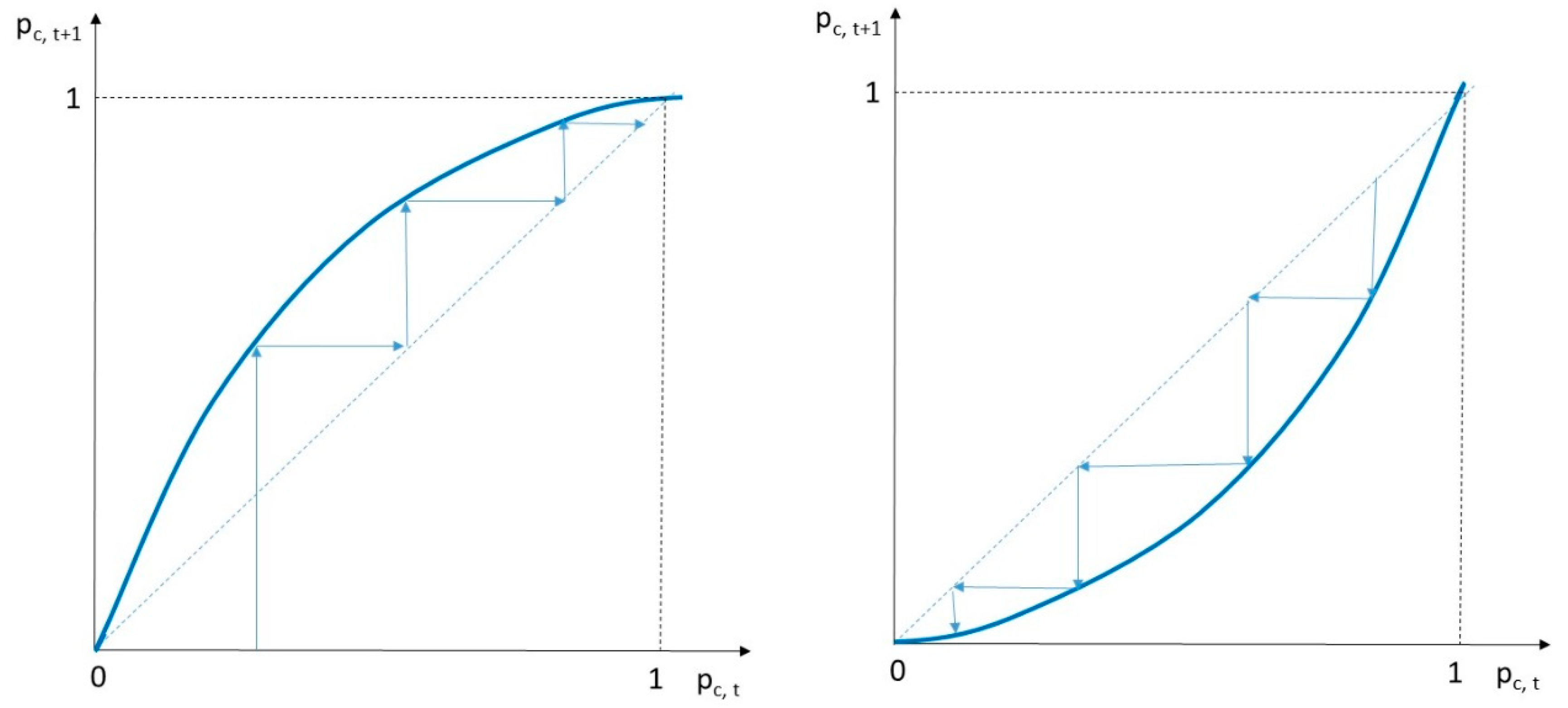
Hence, depending on the expected value of the penalty on the left-hand side of Equation (6), either full tax compliance or a zero tax compliance results (see Figure 1 for the respective tax compliance dynamics). If the expected penalties are high, they render full compliance at a stable fixed point; in contrast, low values of the expected penalties render zero compliance of a stable fixed point. The decisive implication here is that deterministic learning implies an all-or-nothing tax compliance decision of participants.

However, it seems rather unlikely that all or a majority of participants in an experiment behave deterministically. Therefore, a generalization of the learning model is suggested in the following section.

3. Stochastic Learning in Tax Experiments

3.1. Theoretical Analysis

The analysis so far is called deterministic as it employs expected values only, and expected values are fixed numbers. The implication is a deterministic “all-or-nothing” type of taxpaying behavior. This is not in accordance with individual behavior in tax experiments. They show high degrees of volatility concerning tax compliance. In this stochastic version of the deterministic model of Section 1, it is shown that such idiosyncratic and erratic behavior may be caused by a stochastic element of behavior, called “trembling hand”, following Selten [35], and not by irrationality. Put differently, the stochastic mode in this section is a generalization of the former deterministic one.

To incorporate stochasticity, the learning Equation (1) can be formalized as follows ($\rho ≔\frac{\lambda }{Y-A}, \frac{\partial \rho }{\partial \lambda }>0,\frac{\partial \rho }{\partial A}>0, \frac{\partial \rho }{\partial Y}<0)$:

$$\begin{gathered} d{p}_{c\left(t\right)}=\{p_{c\left(t\right)}+p_{c\left(t\right)}·\rho ·T·\left[\left(1-\phi \right)·\left(p_{c\left(t\right)}-1\right)+\left(1-p_{c\left(t\right)}\right)·\phi ·\left(F+1\right)\right]\}·dt \\ +\left[\delta ·\left(1-p_{c\left(t\right)}\right)+\left(1-\delta \right)·p_{c\left(t\right)}\right]°d{W}_t, \delta \in \left(0,1\right) \end{gathered}$$

which can be written as:

$$d{p}_{c\left(t\right)}=p_{c\left(t\right)}\left\{1+\rho ·T·\left(1-p_{c\left(t\right)}\right)·\left[\phi ·\left(F+2\right)-1\right]\right\}·dt+\left[\delta ·\left(1-p_{c\left(t\right)}\right)+\left(1-\delta \right)·p_{c\left(t\right)}\right]°d{W}_t$$

(7)

In Equation (7), the first part up to dt contains the deterministic learning equation with the simplification that the fine F is taken as a fixed number. The second part $\left[\delta ·\left(1-p_{c\left(t\right)}\right)+\left(1-\delta \right)·p_{c\left(t\right)}\right]°d{W}_t$, is the stochastic part. It says that the compliance probability $p_c$ is chosen with a “trembling hand” (Selten [35]). The latter means that with a frequency share of δ, 0 < δ < 1, the decision maker errs or is inattentive when deciding on the income declaration for taxation. This error follows a Wiener process, dW_t. This trembling hand approach renders the dynamical system, defined in Equation (7), a stochastically disturbed system.

The equivalent Ito-equation reads (Reference [36], pp. 235 ff.; Reference [37]):

$$\begin{array}{ll}d{p}_{c\left(t\right)}=\left\{p_{c\left(t\right)}\right\{1& +\rho ·T·\left(1-p_{c\left(t\right)}\right)·\left[\phi ·\left(F+2\right)-1\right]\}\\ & +\frac{1}{2}\left[\delta ·\left(1-p_{c\left(t\right)}\right)+\left(1-\delta \right)·p_{c\left(t\right)}\right]·\left(1-2\delta \right)\}·dt+[\delta ·\left(1-p_{c\left(t\right)}\right)\\ & +\left(1-\delta \right)·p_{c\left(t\right)}]·d{W}_t\end{array}$$

(8)

with

$$\sigma \left(p_{c\left(t\right)}\right):=\delta ·\left(1-p_{c\left(t\right)}\right)+\left(1-\delta \right)·p_{c\left(t\right)}$$

(9)

and

$${\sigma }^{\prime }\left(p_{c\left(t\right)}\right)=1-2\delta$$

(10)

The stationary invariant distribution of the diffusion process defined by Equation (8) with natural boundaries of p_c at zero and unity, as well as $\sigma \left(p_{c\left(t\right)}\right)>0$, is given by Reference [36] (p. 233):

$${\pi }^0\left(p_c\right)=N·\frac{1}{\sigma {\left(p_c\right)}^2}·\exp \left(\underset{c}{\overset{p_c}{{\displaystyle \int }}}\frac{2·p_c\left\{1+\rho ·T·\left(1-p_c\right)·\left[\phi ·\left(F+2\right)-1\right]\right\}}{\sigma {\left(p_c\right)}^2}d{p}_c\right),\forall p_c\in \left(0,1\right)$$

(11)

with normalization factor, N, defined by:

$$N^{-1}:=\underset{0}{\overset{1}{{\displaystyle \int }}}\frac{1}{\sigma {\left(p_c\right)}^2}·\exp \left(\underset{c}{\overset{p_c}{{\displaystyle \int }}}\frac{2·p_c\left\{1+\rho ·T·\left(1-p_c\right)·\left[\phi ·\left(F+2\right)-1\right]\right\}}{\sigma {\left(p_c\right)}^2}d{p}_c\right)dr, \mathrm{with} 0<c<1$$

(12)

Equation (11) can be simplified to:

$${\pi }^0\left(p_c\right)=-N·\exp \left[A\right]·{\left[\delta \left(2p_c-1\right)-p_c\right]}^B$$

(13)

with

$$A:=-\frac{2\left\{p_c\rho T\left(2\delta -1\right)\left[\left(F+2\right)\phi -1\right]-\frac{\delta \left\{\left(\delta -1\right)\rho T\left[\left(F+2\right)\phi -1\right]+2\delta -1\right\}}{\delta +p_c\left(1-2\delta \right)}\right\}}{{\left(2\delta -1\right)}^3}$$

(14)

$$B:=-\frac{1+2\delta \left(1-6\delta +4{\delta }^2\right)+2\rho T\left[\left(F+2\right)\phi -1\right]}{{\left(2\delta -1\right)}^3}$$

(15)

Differentiating Equation (13) with respect to p_c yields:

$$\begin{gathered} \frac{d{\pi }^0\left(p_c\right)}{d{p}_c}=\exp \left(A\right){\left[\delta \left(2p_c-1\right)-p_c\right]}^C\{\delta \left[1-2\delta +4p_c\left(\delta -1\right)\right]-p_c \\ +2p_c\rho T\left[\left(F+2\right)\phi -1\right]\left(p_c-1\right)\} \end{gathered}$$

(16)

$$C≔\frac{1-2\delta \left[7+6\delta \left(2\delta -3\right)\right]-2\rho T\left[\left(F+2\right)\phi -1\right]}{{\left(2\delta -1\right)}^3}$$

(17)

The extrema of the derivative in Equation (16), given by $\frac{d{\pi }^0\left(p_c\right)}{d{p}_c}=0$, are (note that there exists a third extremum outside the range of $p_c\in \left[0,1\right]$):

$$p_{c,1}=\frac{1-4\delta \left(\delta -1\right)+2\rho T\left[\left(F+2\right)\phi -1\right]-\sqrt{{\left(1-4\delta \left(\delta -1\right)\right)}^2+4\rho T\left(1+2\delta \right)\left[\left(F+2\right)\phi -1\right]+4{\rho }^2{T}^2{\left[\left(F+2\right)\phi -1\right]}^2}}{ 4\rho T\left[\left(F+2\right)\phi -1\right]}.$$

(18)

$$p_{c,2}=\frac{1-4\delta \left(\delta -1\right)+2\rho T\left[\left(F+2\right)\phi \right]+\sqrt{{\left(1-4\delta \left(\delta -1\right)\right)}^2+4\rho T\left(1+2\delta \right)\left[\left(F+2\right)\phi -1\right]+4{\rho }^2{T}^2{\left[\left(F+2\right)\phi -1\right]}^2}}{ 4\rho T\left[\left(F+2\right)\phi -1\right]}$$

(19)

For $\delta =0$ (i.e., in the case of deterministic learning), $p_{c,1}=1$ and $p_{c,2}=0$ are the compliance probabilities; these are the same compliance probabilities as in Section 2. Note that the compliance probabilities in Equations (18) and (19) are the most likely values for these probabilities since they are the extrema of the distribution function in Equation (11), with the normalization factor in Equation (12).

Differentiating Equations (18) and (19), respectively, with respect to δ yields:

$$\frac{\partial p_{c,1}}{\partial \delta }=\frac{1-2\delta -\frac{1+2\delta \left(1-6\delta +4{\delta }^2\right)+\rho T\left[\left(F+2\right)\phi -1\right]}{\sqrt{{\left(1-4\delta \left(d-1\right)\right)}^2+4\rho T\left[\left(F+2\right)\phi -1\right]\left\{\left(1+2\delta \right)+\rho T\left[\left(F+2\right)\phi -1\right]\right\}}}}{ \rho T\left[\left(F+2\right)\phi -1\right]}$$

(20)

$$\frac{\partial p_{c,2}}{\partial \delta }=\frac{1-2\delta +\frac{1+2\delta \left(1-6\delta +4{\delta }^2\right)+\rho T\left[\left(F+2\right)\phi -1\right]}{\sqrt{{\left(1-4\delta \left(d-1\right)\right)}^2+4\rho T\left[\left(F+2\right)\phi -1\right]\left\{\left(1+2\delta \right)+\rho T\left[\left(F+2\right)\phi -1\right]\right\}}}}{ \rho T\left[\left(F+2\right)\phi -1\right]}$$

(21)

3.2. Simulations

In the following, the results of the theoretical analysis were used to simulate the size of the effects on the compliance probability by changing parameters. The parameters that are changed are shown in Figure 2, Figure 3, Figure 4 and Figure 5 below, and are (in this order) the “trembling hand” parameter, δ, the learning parameter, $\rho =\frac{\lambda }{Y-A}$, the audit parameter, $\phi$, and the penalty parameter, F.

Figure 2 shows the plot of the most likely tax compliance probabilities from Equation (18) for the following values (note that there is always a second extreme value at p_c = 0 that is not changed by δ in its relevant range): T = 30,000 EUR, F = 3, ϕ = 0.01, and ρ = 0.00001, 0.0001, and 0.001, respectively (from left to right).

Note that the value for the tax liability seems to be adequate for an income of 100,000 EUR a year, and a fine rate of 3 could also be in a realistic range. The same holds probably true for the supposed audit rate of 0.01. The learning parameter is difficult to determine, because it is not observable and it has two crucial aspects: the learning rate, λ, and the aspiration income, A. The parameter values for ρ given above are calculated for a learning rate $\lambda =1$, and values for the distance between the (pretax) income, Y, and the aspiration income, A, because of the tax, Y > A. For instance, $\rho =0.00001$ is compatible with $\lambda =1$, Y = 100,000 EUR, and A = 0 (no income aspiration). The two remaining values of ρ, ρ = 0.0001 and ρ = 0.001, indicate that the aspiration income approaches the pretax income Y. However, it is worth mentioning that the values of ρ given above are also compatible with other combinations of λ and A (for the assumed income of 100,000 EUR).

The diagrams in Figure 2 show how the learning parameter, ρ, influences the most likely compliance probabilities, p_c, for different values of the trembling hand parameter, δ. Small values of ρ imply that the compliance probabilities stay relatively near to their deterministic value of zero. For high values of ρ, the compliance probability remains quite near its other deterministic steady-state value of unity. Nevertheless, the most probable compliance probabilities can deviate to a large extent from both deterministic steady-state values due to the different values of ρ.

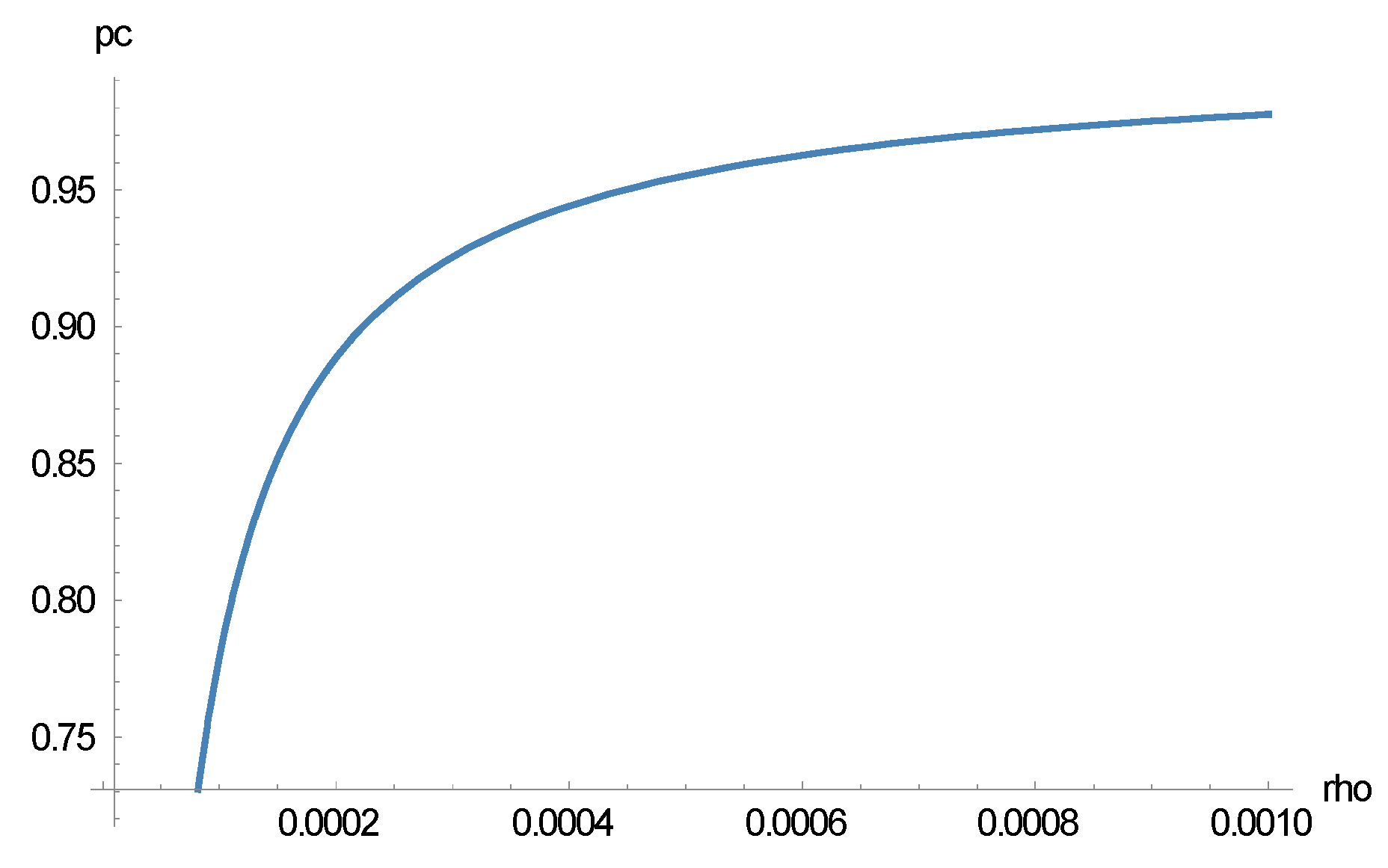
Figure 3 shows the most likely tax compliance from Equation (18) as a function of the learning parameter, ρ, for the following values (note that there is always a second extreme value at p_c = 0 that is not changed by ρ in its relevant range): T = 30,000 EUR, F = 3, ϕ = 0.01, δ = 0.1.

Figure 3 demonstrates that tax compliance increases as the aspiration income increases (with a constant learning rate, λ).

In Figure 4, the most likely tax compliance from Equation (18) as a function of ϕ are depicted for the following values (note that there is always a second extreme value at p_c = 0 that is not changed by ϕ in its relevant range): T = 30,000 EUR, F = 3, ρ = 0.00001, ρ = 0.0001, and ρ = 0.001, respectively (from left to right).

As Figure 4 demonstrates, the effect of the audit on tax compliance depends to a large extent on the learning parameter, ρ. If this parameter is rather low (for instance, because of a low learning rate, λ, or a low aspiration income, A), an increase of the audit rate reduces tax compliance. However, it seems noteworthy to mention that the tax compliance probability decreases with increasing audit rates. This effect is counteracted by the learning parameter, ρ, as is demonstrated in Figure 4 from left to right.

Figure 5 shows the most likely tax compliance from Equation (18) as a function of F for the following values (note that there is always a second extreme value at p_c = 0 that is not changed by F in its relevant range): T = 30,000, ϕ = 0.01, δ = 0.1, ρ = 0.00001, 0.0001, and 0.001, respectively (from left to right).

The effect of a variation of the fine rate, F, too, depends to a large degree on the learning parameter, ρ. The effect is similar to that of a change of the audit rate.

The above results have far-reaching implications for tax and other experiments in economics (and in psychology):

• The most likely compliance probabilities (or propensities) in tax compliance experiments are zero and unity, deterministically, as well as with trembling hand stochasticity;
• Linear approximations of utility functions, in combination with aspiration levels and learning rates, may suffice to explain the experiments’ results.
• “Trembling hands” and learning are seemingly important elements for the explanation of the results of the experiments.
• “Trembling hand” effects cannot be detected with deterministic approaches. The key new insight from the stochastic model is that it captures and explains erratic and idiosyncratic behavioral effects. This implies that participants may not behave irrationally, but only with “trembling hands”.
• Unobservable variables, represented in the above model by the learning rate and the aspiration level, are relevant ingredients in a theory of experimental behavior of human subjects.

4. Empirical Analysis

4.1. Descriptive Analysis

In the following, data from a known and already analyzed tax experiment were used to test empirically whether learning in this abovementioned lab experiment 1 occurred. The reason for using data from this particular experiment was simple: the experiments were run over an unusually large number of 60 rounds each. This number of rounds was sufficiently high to detect learning effects, even if learning was stochastic and slow. This cannot be said in general for experiments that run over 20 rounds, for instance.

The tax experiments consisted of three treatments and were run over 60 rounds each. At the start of each round, in all treatments, the participants received a fixed income of 1000 MU (experimental money units; at the end of the experiment, the remaining MUs were paid out to the participants in Euro, according to a constant and known exchange rate). This exogenously given income was taxable with a lump-sum income tax of 200 MU (i.e., the tax rate was 20%). The participants had to declare their incomes to a “tax authority”. The income declaration was announced to be audited with a probability of 15%. If partial or full tax evasion was detected, the full tax and a penalty had to be paid.

The treatments differed by rewards for paying the tax honestly, i.e., fully. In the first treatment, no reward was paid, whereas in the second (third) treatment, honest taxpayers were paid 200 (400) money units (MUs) if they paid the tax fully. Of course, the reward was only paid in the case that it became evident in an audit that the full income had been declared. Since the audit probability was 15%, in nine of the 60 rounds of the experiment (in round 2, 3, 7, 9, 14, 18, 20, 31, and 51) an audit took place. The fine rate for tax evasion was three times the evaded sum in the first treatment, two times the evaded sum in the second treatment, and one time the evaded sum in the third treatment. These different fine rates were necessary to ensure that the differences in the expected values of full tax compliance and the expected value of full tax evasion remained constant (see Reference [31] for details). In the first and second treatment, 30 persons participated, in the third 26. Hence, the dataset consists of 5160 observations.

After each round of the experiment, the participants’ own round-payoff was communicated to her or him, but not to other participants. The payoff also contained information on whether there was an audit with or without further payments to the tax authority.

The mean and median tax payments over all persons and rounds, presented in

Table 1. Mean and median tax payments according to treatment.

Treatment	Mean Payment	Median Payment	Standard Deviation
No reward	124.96	150.00	82.44
Reward = 200	103.72	105.00	92.97
Reward = 400	139.57	200.00	84.19

Source: Own calculations.

, was the highest in the third treatment and the lowest in the second, with the first treatment in-between. However, individual idiosyncrasies were large in the experiment. Note that it was not intended here to analyze the effects of rewarding honesty in taxpaying; this has already be done in Reference [31]. The focus is here on learning effects only.

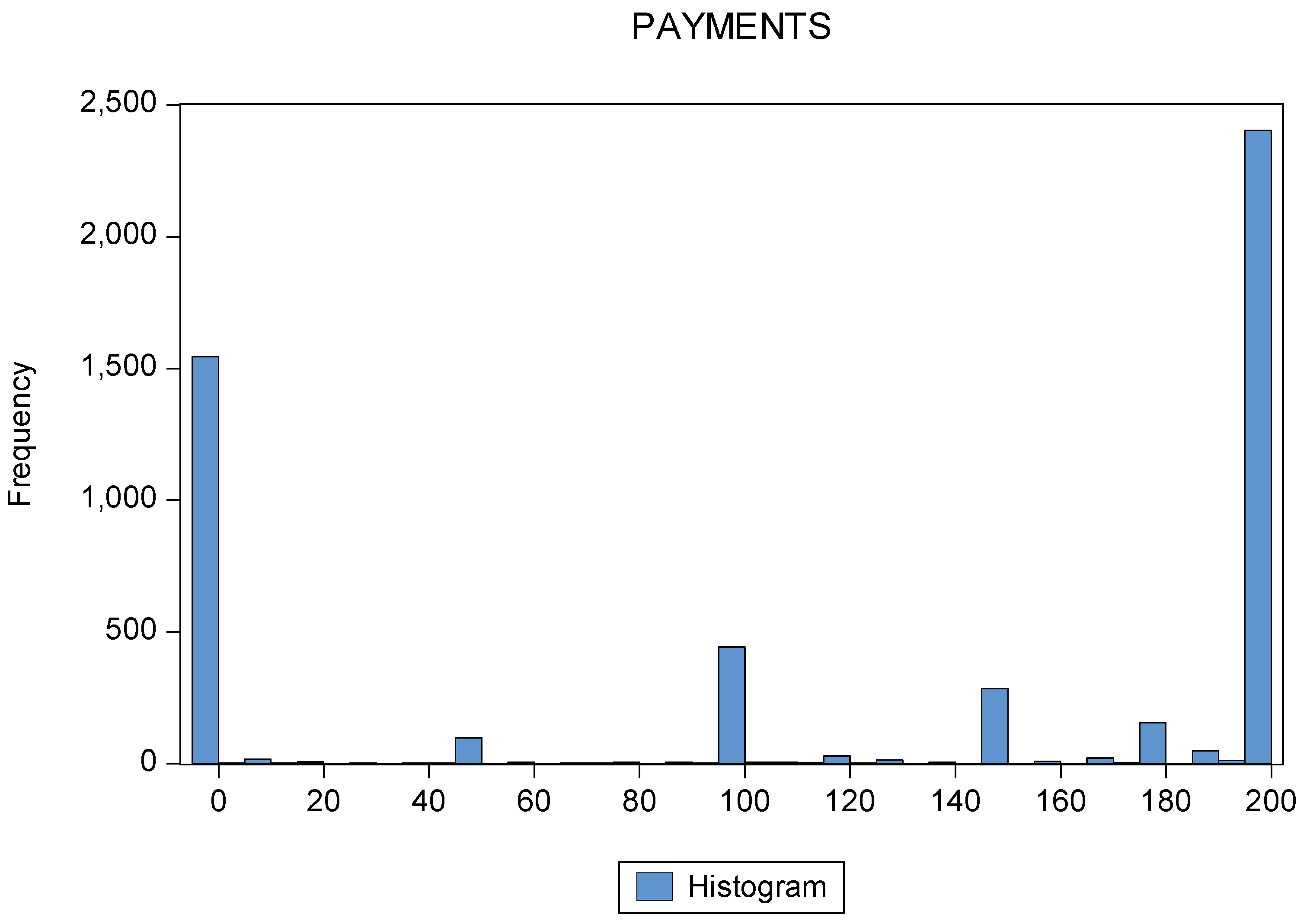
The distribution of all tax payments of all the participants is shown in Figure 6. The most frequent payments are 0 MUs and 200 MUs. However, the distribution seems to have a further local maximum at tax payments of 100 MUs. This may imply that the distribution of tax payments was bimodal.

To check this, the bimodality coefficient, BC, was calculated (Reference [38]; see also Reference [39]):

$$BC=\frac{m_3^2+1}{m_4+3\frac{{\left(n-1\right)}^2}{\left(n-2\right)\left(n-3\right)}}$$

(22)

with m₃ as the skewness of the distribution, m₄ the excess kurtosis (i.e., kurtosis – 3) and n the sample size. The respective values for the distribution of Figure 6 are mean value of payments: 121.97; median payments: 180.00; standard deviation: 87.97; skewness: −0.48, kurtosis: 1.43; and number of observations: 5160. For the distribution in Figure 6, BC = 0.8595. Since this value was larger than the critical value of 5/9 (≈ 0.5555), the distribution was very likely bimodal.

Since in all three treatments the expected value of full tax evasion was 80 MUs higher than the expected value of full tax compliance (including the expected value of the penalty, see Reference [31]), most all-or-nothing taxpaying participants should pay nothing. However, as shown in Figure 6, a majority of participants paid the tax fully. This result may nevertheless be compatible with the theory in Section 2, as idiosyncratic behavior is not considered there. Since the standard deviation of the tax payments in Figure 6 was large (88 MUs, i.e., 72% of the mean tax payment and 49% of the median payment), this may be interpreted in accordance with the stochastic version of the model in Section 3 as a “trembling hand” effect. Of course, this “trembling hand” may also be interpreted as strategically intended by the respective participants to deceive the “tax authority” about their intentions. In a sense, “trembling hands” are a kind of mixed strategy in the game of taxpayers versus the tax authority. As indicated in Figure 2, Figure 3, Figure 4 and Figure 5 above, the income aspiration level and the learning rate play a role for the empirically observable behavior of the participants, although they cannot be observed.

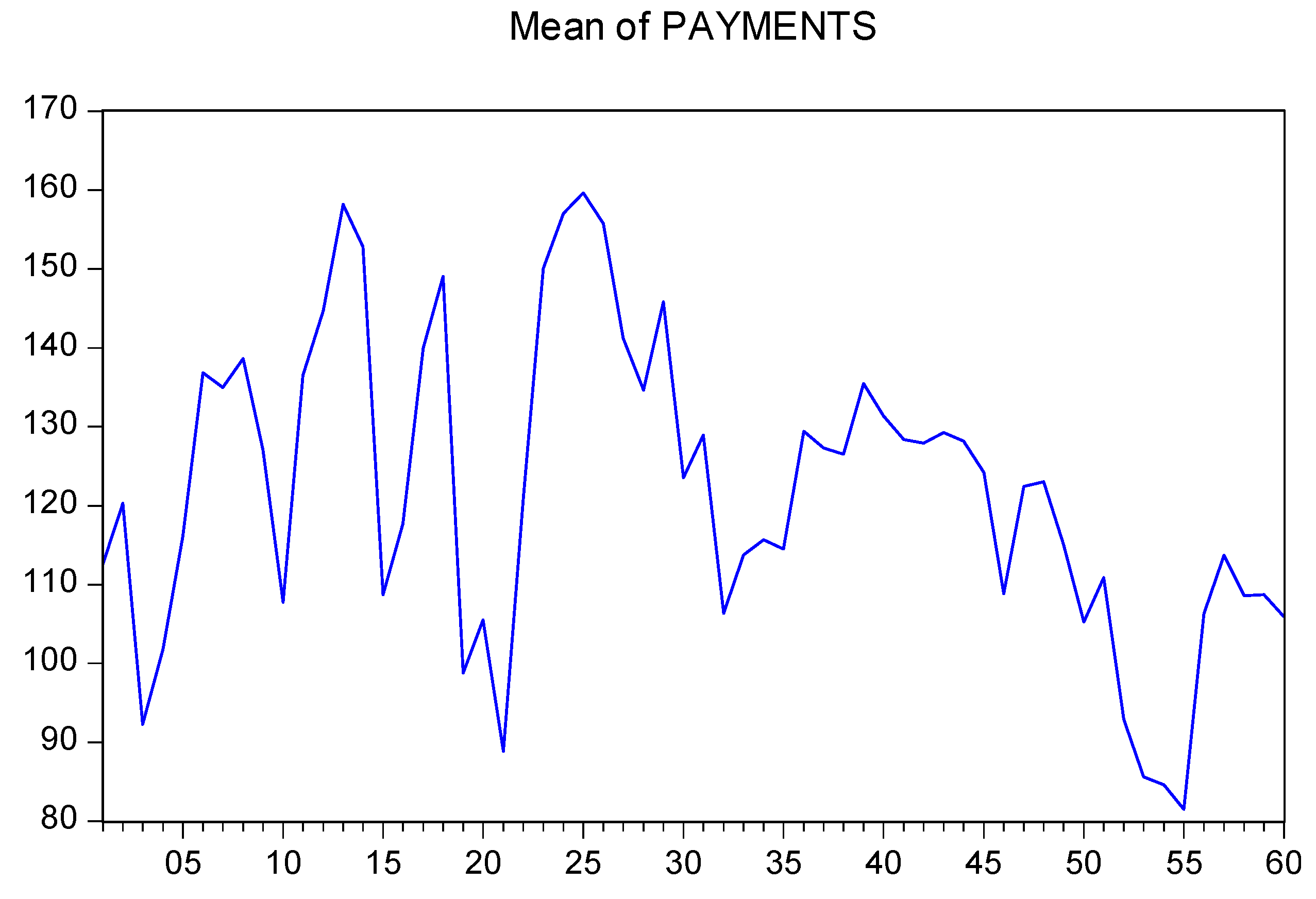
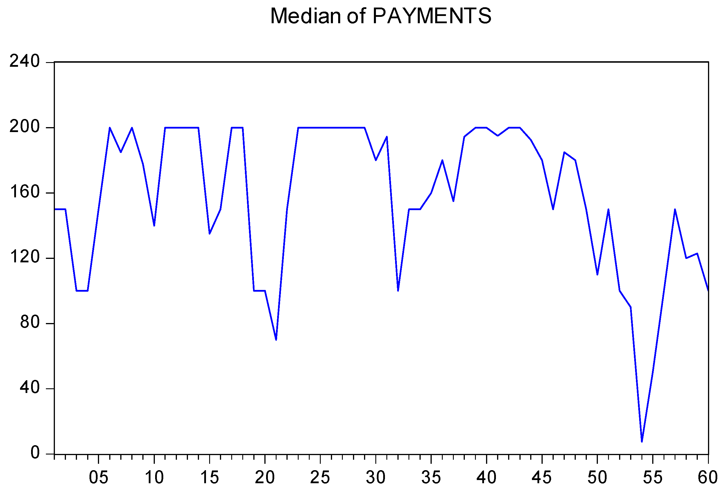
To analyze learning effects over time (i.e., over rounds), Figure 7 and Figure 8 show the mean and median tax payments, respectively, over all rounds by all participants.

It is rather difficult to see whether there is a declining tendency of tax payments over the rounds. The reason is the tremendous individual idiosyncrasies of participants concerning taxpaying. Econometric tests are required to find out whether there is a round-trend in tax payments, as implied by the learning model.

4.2. Econometric Analysis

First of all, learning over the rounds requires that there should be a round trend during the experiment. This was analyzed first. As indicated above, individual idiosyncrasies were large; therefore, participant fixed effects were employed in the estimations of

Table 2. Round trend of tax payments in the different treatments (individual fixed effects).

	Treatment 1		Treatment 2		Treatment 3
Variable	Coefficient	t-Statistic	Coefficient	t-Statistic	Coefficient	t-Statistic
Constant	134.46 ***	41.58	112.40 ***	31.95	155.58 ***	49.09
Trend	−0.32 ***	−3.41	−0.29 ***	−2.86	−0.54 ***	−5.86
Adjusted R2	0.29		0.34		0.43
F-Statistic	25.50 ***		31.84 ***		46.85 ***
Observations	1800		1800		1560

***, **, * Statistically significant at the 1%, 5%, and 10% level, respectively.

. The estimations were separately run for the three treatments (Table 2). In addition, they were also combined and analyzed in

Table 3. Round trend of tax payments (combined treatments).

Variable	Coefficient	t-Statistic
Constant	89.81 ***	8.52
Trend	−0.38 ***	−5.56
Age	1.29 ***	2.87
Sex (female)	30.63 ***	11.63
Treatment = 2	−11.01 ***	−3.50
Treatment = 3	16.87 ***	5.47
Adjusted R2	0.06
F-Statistic	66.19 ***
Observations	5100

***, **, * Statistically significant at the 1%, 5%, and 10% level, respectively.

. In all estimations, “trend” means the dependence of tax payments on the (increasing) number of rounds. If tax payments increase (decrease) with the number of rounds, it is said that there is a positive (negative) trend in tax payments.

Table 2 demonstrates that there are trends in all three treatments of the experiment. The trend of tax payments was negative, i.e., the participants were learning to evade the tax. Since the estimations were run with individual fixed effects, the idiosyncrasies were controlled. Table 3 confirms the negative trend of tax payments (note that the estimation cannot employ individual fixed effects when controlling for the treatments). In addition, the effects differed among treatments. The second treatment (with a reward of 200 MUs for honest taxpaying) generated lower tax payments than the first one (without a reward for honesty), but the third treatment (with a reward of 400 MUs for honest tax paying) generated higher tax payments than the treatment one, but at a budgetary cost.

To analyze the round structure of the trend closer, the 60 rounds of the experiment were separated into three groups with 20 rounds each. As in Table 2, individual fixed effects were employed. The results shown in

Table 4. Trend in round groups and different treatments (individual fixed effects). Dependent variable: tax payments.

	Treatment 1		Treatment 2		Treatment 3		All Participants
Rounds	Trend	t-Statistics	Trend	t-Statistics	Trend	t-Statistics	Trend	t-Statistics
1–20	−0.065	−0.13	0.733	1.38	1.508 ***	3.39	0.689 **	2.37
21–40	0.059	0.12	−0.685	−1.35	−1.220 ***	−2.64	−0.587 **	−2.09
41–60	−2.36 ***	−5.25	−0.698	−1.37	−1.964 ***	−4.43	−1.661 ***	−6.09

***, **, * Statistically significant at the 1%, 5%, and 10% level, respectively.

contain only the trend variable; the values for the estimation constants were not represented to simplify the table. Interestingly, in treatment 2 no statistically significant round-group specific trend can be found. In treatment 1, there was a negative trend in the last 20 rounds only. In treatment 3, there were statistically significant trends in all round groups. However, in the first 20 rounds, the trend of payments was positive, but it turned negative in the two further round groups. As it seems, the overall negative trend in Table 2 and Table 3 originated mainly from the last 20 rounds and additionally from treatment 3. However, as the estimated values with all participants in Table 4 show, the increasing tax compliance in the first 20 rounds was turned around in the following 40 rounds. Moreover, it increased in the last 20 rounds.

The negative round trend of tax payments may be interpreted as a learning effect over the rounds of the experiment. But another effect could also explain the decline of tax payments in the last third of the experiment (with the exception of treatment 3 where the negative trend existed in two-thirds of the rounds). Tiring might be the alternative explanation, as shown by Mead et al. [40] (see also References [21,31]), although it is not fully clear whether the effect was based on being unable or unwilling to declare the correct income, Reference [41]. As already said, tiring might not be the only explanation as the effect existed in the last two-thirds of rounds in the third treatment. Put differently, learning might play a role, even with tiring.

4.3. Robustness Check

To check the robustness of the estimations, tax audits should be considered. If audits change the income declaration considerably, the above result on the statistical significance of round trends—that are interpreted here as indications of learning—might be lost. As was already found with the data used in this paper, there is an impact of audits on taxpaying that was dubbed “bomb crater effect”, References [21,31]. This means that in the round after a tax audit, tax compliance declines. The authors attribute this effect to the so-called “gambler’s fallacy”: individuals found cheating with the tax might react with additional cheating to compensate themselves for the loss. In

Table 5. Audit effects on tax payments (individual fixed effects).

	Treatment 1		Treatment 2		Treatment 3
Variable	Coefficient	t-Statistic	Coefficient	t-Statistic	Coefficient	t-Statistic
Constant	148.09 ***	39.95	120.42 ***	29.42	166.31 ***	45.47
Round = 3	−53.76 ***	−4.16	−38.17 ***	−2.68	−60.93 ***	−4.78
Round = 4	−33.84 ***	−2.63	−31.39 **	−2.21	−58.24 ***	−4.58
Round = 8	−9.21	-0.72	12.76	0.90	−7.86	−0.62
Round = 10	−39.54 ***	−3.10	−34.00 **	−2.41	−17.10	−1.36
Round =15	−43.62 ***	−3.44	−15.06	−1.08	−21.34 *	−1.71
Round = 19	−56.79 ***	−4.50	−29.91 **	−2.15	−14.04	−1.13
Round = 21	−62.79 ***	−4.98	−35.34 **	−2.54	−29.81 **	−2.40
Round = 32	−28.87 **	−2.30	−12.68	−0.92	−15.60	−1.26
Round = 52	−26.40 **	−2.08	−14.60	−1.04	−21.41 *	−1.71
Trend	−0.58 ***	−5.65	−0.45 ***	−3.98	−0.77 ***	−7.52
Adjusted R2	0.32		0.35		0.45
F-Statistic	22.60 ***		25.50 ***		37.26 ***
Observations	1800		1800

***, **, * Statistically significant at the 1%, 5%, and 10% level, respectively.

, the regression results are shown when the “bomb crater effect” is accounted for by control variables for the rounds after a tax audit. Note that all estimations are run with individual fixed effects to control for idiosyncratic behavior.

Most of the round-after-audit dummy variables have a negative and statistically significant sign, but nevertheless the round-trend in all regressions remains negative and statistically significant. This is interpreted as an indication that a learning effect exists that reduces tax compliance.

4.4. Discussion

A general problem with experimental data is that there are a number of individual parameters that cannot be observed. As indicated above, the non-observability of the income aspiration level and the learning rate limits the empirical tests of the learning model. The empirical results do not prove the model, but they are consistent with it.

A great issue is the idiosyncratic and erratic behavior of a large majority of experiment participants. The following effects may provide an explanation for this.

First of all, participants may have a so-called “world model” of the experiment that cannot be known by outside observers [42]. This world model defines how participants understand the tasks of the experiment and what they think about its objectives.

Further effects may exert a crucial influence on the experiment-related behavior of participants, including framing effects [43] and an “experimenter demand” effect [44]. The latter effect says that the behavior in experiments is induced by what participants think that the experimenters are demanding from them. The framing of experiments might give hints to participants what experimenters are demanding from them, i.e., what kind of behavior they should show. Even with no explicit or a “neutral” framing, there is seemingly an “implicit” framing possible [43]. Taken together, the world model, framing, and experimenter demand effects may obscure “real and authentic” behavior. Since these effects have strong idiosyncratic inclinations, they may explain the respective individual behavior in tax compliance (and other) experiments.

Ignoring these effects in the following, it is asked whether the results of the empirical analysis might be interpreted in a different way. As indicated in the introduction, impulsive or automatic behavior and strategic behavior can be distinguished. As demonstrated by Krauskopf and Prinz [32] with data from the experiment employed in this paper, persons who decide very quickly take different decisions in comparison to persons who take time to decide. However, only a small minority takes time to decide. Their number is too small for more general conclusions. Hence, one could say that the results of the experiment demonstrate mainly that the participants decide very differently.

Another interpretation of the results of the experiment could be that they are driven by tiring. As said above, a so-called “ego depletion” effect [40] could be such an explanation. Although the result of the first treatment (without a reward for honest tax paying) supports this interpretation, the result of the third treatment (with a reward of 400 MUs) seems to contradict it since the decline in trend occurs in two-thirds of the rounds of the experiments. It remains unclear, whether it is “ego depletion” or learning (or both) that drives the participants’ behavior.

In effect, the latter result points to a further general issue in experiments. If an experiment encompasses many rounds, making learning possible, the risk is to tire participants into an “ego depletion” effect. Short experiments exclude the latter effect, but it is rather unlikely that strong learning effects occur.

5. Conclusions

In this paper, a theory of learning in games was applied to lab experiments on tax compliance. A theoretical model was provided that can be simulated and tested (at least in principle) with data from experiments.

In the theoretical analysis, two versions of a decision model were developed and analyzed which incorporated learning over time. In the discrete decision model, based on stochastic learning, participants choose the amount of the tax they pay in monetary units. In contrast, an all-or-nothing tax decision model with deterministic learning implies that either no tax or the full tax is paid.

The results of the stochastic model are consistent with experimental data. For example, in the experiment by Kastlunger et al. [31], in 29.9% of all tax payment decisions (5160 cases), the tax was completely evaded, whereas in 46.1% of all decisions, the tax was fully paid. Hence, in 76% of all decisions either no tax or the entire tax was paid. The empirical analysis of the tax payment distribution indicates that the distribution seems to be bimodal, but with considerable variance.

The results of the econometric analysis showed that there was a tendency for participants to learn to evade tax payments over the rounds of the experiment. Controlling for idiosyncratic and erratic individual behavior by fixed individual effects, a statistically significant negative payment round trend was detected. The learning interpretation of this trend was contrasted with a tiring or “ego depletion” effect. Albeit participants of the first treatment showed the negative payment trend only in the last third rounds of the experiment, the participants of the third (rewarded) treatment reduced their tax payments over two-thirds of the rounds. The conclusion in this paper is, therefore, that the negative payment trend over the rounds may indicate a systematic learning effect.

As a general conclusion, it may be said that the idiosyncratic behavior of participants in lab experiments is creating a substantial level of statistical noise that makes it difficult to interpret the data of tax experiments. Nonetheless, a stochastic learning approach seems adequate to analyze these data.

References

1. Allingham, M.G.; Sandmo, A. Income tax evasion: A theoretical analysis. J. Public Econ. 1972, 1, 323–338. [Google Scholar] [CrossRef]
2. Yitzhaki, S. Income tax evasion: A theoretical analysis. J. Public Econ. 1974, 3, 201–202. [Google Scholar] [CrossRef]
3. Torgler, B. Speaking to theorists and searching for facts: Tax morale and tax compliance in experiments. J. Econ. Surv. 2002, 16, 657–683. [Google Scholar] [CrossRef]
4. Mascagni, G. From the lab to the field: A review of tax experiments. J. Econ. Surv. 2018, 32, 273–301. [Google Scholar] [CrossRef]
5. Hashimzade, N.; Myles, G.D.; Tran-Nam, B. Applications of behavioral economics to tax evasion. J. Econ. Surv. 2013, 27, 941–977. [Google Scholar]
6. Luttmer, E.F.P.; Singhal, M. Tax morale. J. Econ. Perspect. 2014, 28, 149–168. [Google Scholar] [CrossRef]
7. Pickhardt, M.; Prinz, A. Behavioral dynamics of tax evasion. A survey. J. Econ. Psychol. 2014, 40, 1–19. [Google Scholar] [CrossRef]
8. Slemrod, J. Tax Compliance and Enforcement. NBER 2018. [Google Scholar] [CrossRef]
9. Ariely, D. The (Honest) Truth about Dishonesty; HarperCollins: New York, NY, USA, 2012. [Google Scholar]
10. Mazar, N.; Amir, O.; Ariely, D. The dishonesty of honest people: A theory of self-concept maintenance. J. Marketing Res. 2008, 45, 633–644. [Google Scholar] [CrossRef]
11. Cross, J.G. A stochastic learning model of economic behavior. Q. J. Econ. 1973, 87, 239–266. [Google Scholar] [CrossRef]
12. Börgers, T.; Sarin, R. Learning through reinforcement and the replicator dynamics. J. Econ. Theory 1997, 77, 1–14. [Google Scholar] [CrossRef]
13. Erev, I.; Roth, A.E. Predicting how people play games: Reinforcement learning in experimental games with unique, mixed strategy equilibria. Am. Econ. Rev. 1998, 88, 848–881. [Google Scholar]
14. Goeree, J.; Holt, C.A. Stochastic game theory: For playing games, not just for doing theory. PNAS 1999, 96, 10564–10567. [Google Scholar] [CrossRef] [Green Version]
15. Fudenberg, D.; Levine, D.K. The Theory of Learning in Games; MIT Press: Cambridge, UK, 1998. [Google Scholar]
16. Fudenberg, D.; Levine, D.K. Whither game theory? Towards a theory of learning in games. J. Econ. Perspect. 2016, 30, 151–169. [Google Scholar] [CrossRef]
17. Neiman, T.; Loewenstein, Y. Reinforcement learning in professional basketball players. Nat. Commun. 2011, 2, 569. [Google Scholar] [CrossRef] [Green Version]
18. Spanknebel, M.; Pawelzik, K. Dynamics of human cooperation in economic games. Available online: https://arxiv.org/abs/1508.05288 (accessed on 27 September 2019).
19. Vale, R. A model for tax evasion with some realistic properties. Available online: https://arxiv.org/pdf/1508.02476.pdf (accessed on 27 September 2019).
20. Soliman, A.; Jones, P.; Cullis, J. Learning in experiments: Dynamic intraction of policy variables designed to deter tax evasion. J. Econ. Psychol. 2014, 40, 175–186. [Google Scholar] [CrossRef]
21. Kastlunger, B.; Kirchler, E.; Mittone, L.; Pitters, J. Sequences of audits, tax compliance, and taxpaying strategies. J. Econ. Psychol. 2009, 30, 405–418. [Google Scholar] [CrossRef]
22. DeBacker, J.; Heim, B.T.; Tran, A.; Yuskavage, A. Once bitten, twice shy? The lasting impact of enforcement on tax compliance. J. Law Econ. 2018, 61, 1–35. [Google Scholar] [CrossRef]
23. Kogler, C.; Mittone, L.; Kirchler, E. Delayed feedback on tax audits affects compliance and fairness perceptions. J. Econ. Behav. Organ. 2016, 124, 81–87. [Google Scholar] [CrossRef]
24. Muehlbacher, S.; Mittone, L.; Kastlunger, B.; Kirchler, E. Uncertainty resolution in tax experiments: Why waiting for an audit increases compliance. J. Socio-Econ. 2012, 41, 289–291. [Google Scholar] [CrossRef]
25. Gangl, K.; Torgler, B.; Kirchler, E.; Hofmann, E. Effects of supervision on tax compliance: Evidence from a field experiment in Austria. Econ. Lett. 2014, 123, 378–382. [Google Scholar] [CrossRef]
26. Mittone, L.; Saredi, V. Commitment to tax compliance: Timing effects on willingness to evade. J. Econ. Psychol. 2016, 53, 99–117. [Google Scholar] [CrossRef]
27. Mittone, L. Dynamic behaviour in tax evasion: An experimental approach. J. Socio-Econ. 2006, 35, 813–835. [Google Scholar] [CrossRef]
28. Maciejovsky, B.; Kirchler, E.; Schwarzenberger, H. Misperception of chance and loss repair: On the dynamics of tax compliance. J. Econ. Psychol. 2007, 28, 678–691. [Google Scholar] [CrossRef]
29. Kirchler, E.; Hoelzl, E.; Wahl, I. Enforced versus voluntary tax compliance: The „slippery slope“ framework. J. Econ. Psychol. 2008, 29, 210–225. [Google Scholar] [CrossRef]
30. Prinz, A.; Muehlbacher, S.; Kirchler, E. The slippery slope framework on tax compliance: An attempt to formalization. J. Econ. Psychol. 2014, 40, 20–34. [Google Scholar] [CrossRef]
31. Kastlunger, B.; Muehlbacher, S.; Kirchler, E.; Mittone, L. What goes around comes around? Experimental evidence of the effect of rewards on tax compliance. Public Financ. Rev. 2011, 39, 150–167. [Google Scholar] [CrossRef]
32. Krauskopf, T.; Prinz, A. Methods to reanalyze tax compliance experiments: Monte Carlo simulations and decision time analysis. Public Financ. Rev. 2011, 39, 168–188. [Google Scholar] [CrossRef]
33. Srinivasan, T.N. Tax evasion: A model. J. Public Econ. 1973, 2, 339–346. [Google Scholar] [CrossRef]
34. Güth, W. Satisficing and (un)bounded rationality—A formal definition and its experimental validity. J. Econ. Behav. Organ. 2010, 73, 308–316. [Google Scholar] [CrossRef]
35. Selten, R. Re-examination of the perfectness concept for equilibrium points in extensive games. Int. J. Game Theory 1975, 4, 25–55. [Google Scholar] [CrossRef]
36. Jetschke, G. Mathematik der Selbstorganisation; VEB Deutscher Verlag der Wissenschaften: Berlin, Germany, 1989. [Google Scholar]
37. Pontryagin, L.; Andronov, A.; Vitt, A. On the statistical treatment of dynamical systems. In Noise in Nonlinear Dynamical Systems. Vol. 1: Theory of Continuous Fokker-Planck Systems; Moss, F., McClintock, P.V.E., Eds.; Cambridge University Press: Cambridge, UK, 1989; pp. 329–348. [Google Scholar]
38. Pfister, R.; Schwarz, K.A.; Janczyk, M.; Dale, R.; Freeman, J.B. Good things peak in pairs: A note on the bimodality coefficient. Front. Psychol. 2013, 4, 1–4. [Google Scholar] [CrossRef] [PubMed]
39. Freeman, J.B.; Dale, R. Assessing bimodality to detect the presence of a dual cognitive process. Behav. Res. Methods 2013, 45, 83–97. [Google Scholar] [CrossRef]
40. Mead, N.L.; Baumeister, R.F.; Gino, F.; Schweitzer, M.E.; Ariely, D. Too tired to tell the truth: Self-control resource depletion and dishonesty. J. Exp. Soc. Psychol. 2009, 45, 594–597. [Google Scholar] [CrossRef] [Green Version]
41. Wu, S.; Peng, M.; Mei, H.; Shang, X. Unwilling but not unable to control: Ego depletion increases effortful dishonesty with material rewards. Scand. J. Psychol. 2019, 60, 189–194. [Google Scholar] [CrossRef] [PubMed]
42. Shteingart, H.; Loewenstein, Y. Reinforcement learning and human behavior. Curr. Opin. Neurobiol. 2014, 25, 93–98. [Google Scholar] [CrossRef] [PubMed] [Green Version]
43. Engel, C.; Rand, D.G. What does “clean” really mean? The implicit framing of decontextualized experiments. Econ. Lett. 2014, 122, 386–389. [Google Scholar] [CrossRef]
44. Zizzo, D.J. Experimenter demand effects in economic experiments. Exp. Econ. 2010, 13, 75–98. [Google Scholar] [CrossRef]
1
The experiment was documented and analyzed in Kastlunger et al. [31], as well as in Krauskopf and Prinz [32]. The entire dataset of the experiment was kindly provided by Erich Kirchler and Stephan Muehlbacher.
Figure 1. Tax compliance dynamics. Diagram on the left: full tax payment; diagram on the right: no tax payment.
Games 10 00038 g001
Figure 2. Tax compliance probability, pc, as a function of the trembling hand parameter, δ, for different values of ρ: (a) ρ = 0.00001, (b) ρ = 0.0001 and (c) ρ = 0.001.
Games 10 00038 g002
Figure 3. Tax compliance probability, pc, as a function of ρ.
Games 10 00038 g003
Figure 4. Tax compliance probability, pc, as a function of ϕ for different values of ρ: (a) ρ = 0.00001, (b) ρ = 0.0001 and (c) ρ = 0.001.
Games 10 00038 g004
Figure 5. Tax compliance probability, pc, as a function of F for different values of ρ: (a) ρ = 0.00001, (b) ρ = 0.0001 and (c) ρ = 0.001.
Games 10 00038 g005
Figure 6. Distribution of tax payments, all participants. Source: Own calculations.
Games 10 00038 g006
Figure 7. Mean tax payments, rounds 1 to 60, of all participants. Source: Own calculations.
Games 10 00038 g007
Figure 8. Median tax payments rounds 1 to 60 of all participants. Source: Own calculations.
Games 10 00038 g008